A Class of Three-Dimensional Optimum Wings in Hypersonic Flow

A CLASS O F T H R E E DIMENSIONAL OPTIMUM WINGS

I N HYPERSONIC FLOW

T h e s i s by

T s e - F o u Zien

In P a r t i a l Fulfillment of the Requirements:

F o r the Degree of Doctor of PhiPos ophy

California Institute of Technology Pasadena, Calif o r nia

19 $7

Acknowledgment

I am g r e a t l y indebted t o Professor J u l i a n D. Cole who, i n addi- t i o n t o p r w i d i n g guidance t o my research i n general, suggested t h i s problem i n p a r t i c u l a r and gave constant advice and encouragement throughout t h e i n v e s t i g a t i o n . Various d i f f i c u l t i e s i n t h e present study were w e r c m e through numerous s t i m u l a t i n g discussions with him. My a s s o c i a t i o n with him i n t h e s e four years a t t h e C a l i f o r n i a I n s t i t u t e of Technology has indeed made t h i s last p a r t of my student's l i f e t h e most enjoyable and memorable.

Thanks a r e a l s o due t o Kiku Matsmots f o r h e r a s s i s t a n c e i n t h e numerical progrc~wning; t o Viv Pfckelsimer f o r h e r excellene typing of t h e t h e s i s ,

It i s a g r e a t pleasure t o express angr g r a t i t u d e t o my dear parents who have given me encouragement and support i n a l l r e s p e c t s during

t h e e n t i r e course of my graduate study.

L a s t l y , but n o t Beastly, 1 wish t o record my deep a p p r e c i a t i o n t o my wife, Suzy Shern, whose understanding and u n f a i l i n g encourage- ment contributed t h e most t o t h e success of my graduate study.

Abstract

The idea of using streamlines of a certain known flow field

to construct generally three-dimensional lifting surfaces together

with the method of evaluating the aerodynamic forces on the sur-

faces, developed by Nonwefler, Jones and Woods, has been extended

and applied to axisymmetric hypersonic flow fields associated with

n

a class of slender power-law shock waves of the f o m r

-

TX in the limit of infinite free stream Mach number. For this purpose,

the basic %Pow fields assoctated with concave shocks (n > 1) have

first been calculated mumerfcafly at a fixed value sf the ratio

of specific heats y = 1.40, and the results are presented in tabu-

lated f o m , covering a wide range! sf values sf m e The method of

constructing a lifting surface either by prescribing its leading

edge shape on the basic shock or by specifying its trailing edge

shape in the plane x = P is then discussed. Expressions for lift and drag on the surface are derived. A class of sptiwwrn shapes

giving m i n i m pressure drag at a fixed value sf lift has been

-iv-

Table of Contents

Acknowledgments A b s t r a c t

Table of Contents L i s t of F i g u r e s L i s t of Symbols

I Introduction 1

I1 Solution of the Hypersonic S m a l l Disturbance Equations f o r the A x i s y m m e t r i c Flow A s s o c i a t e d with a Power-Law Shock 5

2.1. F ~ r m u l a t i o n of the P r o b l e m 5 2.1.1 Derivation of the Limiting HSDT Equations 5 2.1.2 Special C l a s s of S i m i l a r i t y Solutions

-

Power-Law Shock 10

2.2 Behavior of the Solution Near t h e Body Surface 2 1

2.3 N u m e r i c a l Integration of the Differential Equations 2 4 G e o m e t r i c a l and Aerodynamic P r o p e r t i e s of the Lifting Surface 3 0

3.1 G e n e r a l Considerations 3 0

3.2 The E x p r e s s i o n of the S t r e a m Function 3 2 3.3 G e o m e t r y of the Lifting Surface 3 3

3.3. B Lifting Surface with P r e s c r i b e d Leading

Edge. An Example 3 4

3 . 3 . 2 Lifting Surface with P r e s c r i b e d T r a i l i n g

Edge, An Example 41

3-4 Aerodynamic F o r c e s on the Lifting Surface 48

3.4. B D i r e c t Method 48

3.4.2 Indirect Method 50

IV

Optimum Shapes

4.1 G e n e r a l Discussions

4.2 C o n s t r a i n t s

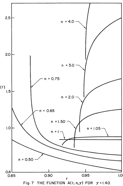
4.2. P I s o p e r i m e t r i c Constraint 4.2.2: Differential C o n s t r a i n t 4.3 The Role of the Function A(T)

4.4 BptirnumShapes f o r

%

< n < < . y = 1 , 4 0 4.5 Optimum Shape f o r n = 1, y = 1.40

4.6 O p t i m u m S h a p e s f o r n > P , y = B . 4 8 4.6.1 C a s e P < n < 1.065

4.4.2 C a s e n

>

1.065 4.7 ConclludingRemark Appendix

Table

[image:4.530.40.481.262.725.2]

L i s t of Figures

Number Page

Coordinate Systems

...

97

Numerical Solution

-

Pressure F i e l d ( y = 1.40)

...,

98

Numerical Solution

-

Velocity F i e l d (y = 1.48) oe... 99

NumericaP Solution

-

Density F i e l d (y = 1.48)

...

100

ControB Volume ~ . . . . . . . . . . . . . . ~ e. . P D O~ ~ ~ . O~ D D D e O~ . eP PO O 101 The Curve ~ ' ( l ; n , y ) = 0 f o r Y = 1.40

..

...

102

The Function A(l;n,Y) f o r y = 1.40 . e . . e e . . O . O . . . s s . D e 103 Graphical Solution f o r hl a e . . ~ ~ ~ o ~ ~ ~ ~ e104 ~ e e e ~ ~ e ~ ~ ~ ~ e o ~ ~ DA and LA f o r y = 1.40

...

105

h 2 ( r ) f o r y = 1.40

...

106

T r a i l i n g Edge Shape and Leading Edge P r o j e c t i o n s f t h e Optimum Shape n = 1

...

PO7 T r a i l i n g Edge Shape and Leading Edge P r o j e c t i o n sf t h e Optirwm Shape n = 3/4

...,,.

108

T r a i l i n g Edge Shape and Leading Edge P r o j e c t i o n of t h e Optimum Shape n = 1/2

.

.

. .

. .

..

.

.

.

. .

.

.

.

. .

, ,... 109 Planforms of the BptPmum Shapes n = 1.0, 314 e * .

.

e n , 110

PPanBom and Center kine of t h e Optimum Shape

List of Symbols

A =

& I 3

(Eq. 4.5)

B = equation of lifting surface C = elevation of the leading edge

D = drag integral (Eq. 3.41)

G = r/xn

-

G = r

2

II = hypersonic similarity parameter 1 4 6

,

also functional of variational problems

L = lift integral (Eq. 3.421, also leading edge function

QEq. 3.9)

P = pressure similarity function (Eq. 2.4Qb) C

! = d@(r)/dr (Eq, 4.44

R = density similarity function (Eq. 2.40~)

*

S = shock function, leading term of g(x

T

= side thrust integral, temperature field, also D/L

V

= velocity similarity functim (Eq. 2,40a) a = speed of sound

b = body shape factor f = body shape function

g = shock shape function

4-99

(i,j,k) = unit vectors of the Cartesian coordinate system

(kl,k2)

= elevation of trailing edge

n n = exponent, S(x) = x

-b

q = velocity vector

r = distance from the axis of synnnetry

s = area

u = non-dimensional axial velocity component

v = non-dimensional transverse velocity component (x,y,z) = cartesian coordinates system

CY = invaiiant coordinate (Eq. 2.41)

p = Pnvariant coordinate (Eq. 2,411

y = specific heats ratio

6 = characteristic shock angle, also variation

T/ = similarity variable, 2 ~ 1 ~ ~ ~

-

7] = basic similarity variable r/xm

*

*

( h h ) = Eagrange multipliers

I s

2

6

= auxiliary coordinate (Eq. 2,421

%

= auxiliary coordinate,+ (Eq. 2,421 p = density

*

H=

= control surface

= non-dimemsiona4 density

T = thickness parameter

@ = azimuthal angle

Y

= stream function

= lifting surface

2

s lift function

Subscripts

=

= conditions upstream of the shock wave

s = conditions downstream of the shock wave b = conditions on the body surface

Superscripts

I. Introduction

Recent advances in technology have made flight at hypersonic speeds

realizable. As a consequence, the practical problem of the optimum de-

sign of the aerodynamic shapes in this speed range is beginning to at-

tract considerable attention from many aerodynamicists, and significant

progress has been achieved. Perhaps the most up-to-date survey of the

current status of this subject is given by Miele. -ever, most of

the available analyses seem to be restricted to two dimensional or axi-

symmetric shapes; also the Newtonian approximation sf pressure distri-

bution is widely adopted in the analyses. The treatment of general

three dimensional shapes without the simplifying assumption of Newtonian

pressure distribution appears to be fomidable because of the inherent

difficulties of solving the strongly non-linear set of equations of

gasdynamics in any generality. This is true even for slender shapes

where the simplified equations of the hypersonic small disturbance

theory (henceforth referred to as HSDT) can be successfully applied.

Nevertheless, a relatively new method of constructing lifting

surfaces within the framework of inviscid gasdynamic theory has re-

cently been developed. This method furnishes a fairly wide class of

three dimensional surfaces whose aerodynamic characteristics can be

determined exactly. This method, first developed by Nonweiler, (2) consists of using the streamlines in some basic known flow field as

the elements sf the surface. If an arbitrary e u m e prescribed on the

shock surface sf the basic flow field is taken as the leading edge of

the lifting surface, then the BiftPng surface is f o m d by those

s t r e a m l i n e s t h a t p e n e t r a t e t h e b a s i c shock s u r f a c e through t h e p o i n t s

on t h e l e a d i n g edge curve. Obviously t h i s l i f t i n g s u r f a c e w i l l have

a shock wave of known shape a t t a c h e d a l l along i t s l e a d i n g edge. That part of t h e o r i g i n a l flow f i e l d between t h e l i f t i n g s u r f a c e and t h e

shock wave a t t a c h e d a l o n g i t s l e a d i n g edge w i l l remain u n a l t e r e d regard- l e s s of t h e replacement of t h e o r i g i n a l body by t h e l i f t i n g s u r f a c e .

T h e r e f o r e , t h e f o r c e s a c t i n g on t h e s u r f a c e a r e a c c e s s i b l e t o e x a c t

c a l c u l a t i o n s . Nonweiler i l l u s t r a t e d t h e i d e a by t a k i n g t h e flow f i e l d

behind a plane o b l i q u e shock wave generated by a two dimensional wedge

f l y i n g a t supersonic speeds a s t h e b a s i c flow f i e l d . E a t e r Jones ( 3 )

and Woods ' 4 9 5 ' c a r r i e d t h e i d e a wet t o t h e c a s e where an a x i s m e t r i c supersonic cone f i e l d i s taken a s t h e b a s i c f i e l d . They i n d i c a t e d a procedure of c o n s t r u c t i n g t h e s u r f a c e gebfnetrically a s w e l l a s a method

of numericaPly e v a l u a t i n g t h e aerodynamic f o r c e s om i t .

It now seems f e a s i b l e t o g e n e r a t e a f a i r l y wide c l a s s of t h r e e d i - mensional l i f t i n g s u r f a c e s from some known two dimensional o r axisym- m e t r i c flow f i e l d s . The same i d e a can e q u a l l y w e l l be a p p l i e d t o hyper- s o n i c flow f i e l d s and hence t o t h e d e s i g n of a c l a s s of t h r e e dimen-

s i o n a l hypersonic l i f t i n g s u r f a c e s . I n both t h e supersonic and t h e hy-

p e r s o n i c c a s e s , t h e s o l u t i o n t o t h e b a s i c flow f i e l d i s e s s e n t i a l , Among t h e l i m i t e d number of e x i s t i n g e x a c t s o l u t i o n s t o t h e equa-

t i o n s of hypersonic small d i s t u r b a n c e t h e o r y , t h e s e l f - s i m i l a r flow be-

*n

hind an anxisymmetric power-law shock wave s f t h e f o m r*

-

TX

,

seems t o be t h e most i n t e r e s t i n g one f o r t h i s purpose, h d e t a i l e d account

which the discussion is limited to the non-concave shapes of the body

and shock only, i.e., n S 1. Extensive numerical results for the cor-

responding flow field have also been tabulated in ~ h e r n ~ i ( ~ ) and Gersten

and Nicolai. (8) For concave shapes, the flow field also exhibits simi-

larity, but the only investigation considers a two dimensional case

(~ullivan")). The numerical calculations for the corresponding axi-

symmetric case do not seem to exist in the literature.

In the present thesis, the previously mentioned method of construct-

ing the lifting surface is extended and applied to the limiting hyper-

sonic small disturbance flow field (i.e., H s 0) associated with an

*

*n

axisymmetric slender power Paw shocks of the form r .-ax for all n

greater than 112. The surfaces under consideration have the following

general properties: (1) the trailing edge when projected onto the plan

is straight a ~ d perpendicular to the axis of symmetry of the basic

field, (2) the leading edge is on the original shock surface and is

symmetric with respect to a meridian plane of the basic axismetric

field. To do this, the numerical solutions of the concave shock case

are first obtained in Chapter 2 by reformulating the problem in terms

of similarity variables and then solving it numerically on the IBM 7094

digital computer for y = 1.40 and a wide range of an. Certain singular behavior sf the solution is noted and discussed. Then in Chapter 3,

the geometrical construction of the surface is discussed in detail for

both the case sf prescribed leading edge shape and for the case sf pre-

scribed trailing edge shape. The method of calculating the lift and

the forces are given in terms of single integrals. The integrals are

in the trailing edge plane and involve a function which characterizes

the shape of the trailing edge. A variational problem is then fomu-

lated and solved in Chapter 4 to find an optkmm family of shapes which,

for a given set of values of n and y, gives minimum drqg for a fixed

lift. Certain geometrical constraints derived from some practical con-

siderations arise naturally. Typical. results on the optimum shapes

and the associated formulae for the minimum drag are also presented,

covering a wide range sf n for y = l,4.

It is to be noted here that the treatment sf the problem in gen-

eral supersoni~ case is possible for the exceptional value sf n equal

to unityo i.e.,'the axisymmetric cone field, simply because of the fact

that exact solution of the flow field is available for that exceptional case without using the approximations of HSDT. However, calculations

would then have to be made for every set of values of M and Bs (or

w

Bb). the half shock cone angle (or half body cone angle). By study- ing the limiting case of hypersonic flow corresponding to M = w , the

w

11. Solution of the Hypersonic Small Disturbance Equations for the Axisyrmnetric Flow Associated With A Bower-Law Shock

2.1. Formulation of the Problem.

In this section, the limiting HSDT equations and boundary condi-

tions are derived from the exact, inviscid gasdynamic equations and

shock wave relations as well as the conditions of tangential flow on

the body surface. Next, specialization to the class of the flow asso-

ciated with power-law shape of shock wave is made and the similarity

formulation of the problem is given.

(2.1.1) Derivation of the Limiting HSDT Equations.

The derivation of the HSDT equations is well-known (see, for ex-

ample, Van ~~ke"~)) ; however, it is included here for completeness.

Consider the steady, uniform flow of a stream of calorically per-

fect gas at Mach number Moo w e r a slender body of revs%ution of the

form

*

*

where x and r are the streamwise and transverse coordinates respec-

tively, and T is a small parameter characterizing the body surface in-

elination to the free stream.

As LO workPng hypothesisg the associated shock wave shape is pos-

-6-

Let the quantity 6 be defined as a characteristic angle which the

shock wave makes with the free stream, i.e.,

d

*

d

*

2

tan 6 = '-3; g(x ,T) = T 7 S(x)

+

O(T ) . (2 3)

dx dx

Since T -r 0, (2.3) implies that the angle also tends to zero uni-

*

formly if ~'(x ) is uniformly of O(1) throughout the flow field.

We now consider the following limit:

The equations of motion derived from the exact, inviscid gasdy-

namie equations under the limit (2.4) are the limiting WDT equations.

It is to be noted here that in the class of problem considered later,

the assumpti ons (2.4) underlying the approximati on may break down

locally and thus results in certain singular behavior of the solutions.

More explicitly, for the class sf flow where'

*

the assumption of small flow deflection 6 -r 0 breaks down at x = o

*

for w < 1 because S '(x ) = Q) there On the other hand, the assumption

*

of strong shock 1 1 2 6 ~ = 0 is violated at x = o for n > 1 because 0)

~'(x*) = O at the tip. These singularities will be discussed later.

*

We d l 1 assume here that

s

'(x ) f s generally of O ( B ) except for

The physical interpretations of the limit (2.4) are as follows.

The limit Mw 4 m corresponds to the case that the free stream sound

speed am 4 o while the free stream density pw and speed Um are kept

fixed, or equivalently, the ambient pressure pm and temperature Tm

tend to zero. The limit 6 -, 0 (or T -, 0) corresponds to the case of

small flow deflection. The strong shock limit 1 / 4 6 ~ = 0 (or

1 / G 2 = 0) indicates the fact that the free stream Mach angle vanishes

faster than the local shock wave angle does, because the product Mm6

can be interpreted as the ratio of the characteristic shock angle to

the free stream Mach angle.

In carrying out this limiting process, the strained coordinates

*

i

P = P / T ~ x = x are used and kept fixed in order to keep the relative position of a field point and the body surface invariant.

The exact conditions across the shock wave in uniform stream can

*

u - U s W

e:-

U 01 Y + l sin2 1

[1

- (

Ma sin 6

)2]

(2.5d)

where the subscripts w and s represent conditions on the upstream and

downstream sides of the shock surface respectively.

A study of Eqs. (2.5) under the limit (2.4) suggests the following

representations of the exact flow fields:

where the fact that lim 617 = 0(l) is used and the velocity field

G*

+*

*

*

* * *

isrepresentedbyq ( x , r , ~ ) = U ~ ~ ~ u ( ~ ~ r , ~ ) + ~ ~ v * ( ~ * , r * ~ ~ ] . .

The exact kquations of steady motion of an inviscid, nmconduct-

Png gas in an ax%symmetrfc field are:

a

* * *

a

* * *

continuity: _{7 (p u r )}

+

_{7 (p v r ) = O} (2.4a)

ax

a r

*

2

axial momentum: u 7

*

₇

auk

+

_{* 2} 1

=

a,*

*

o

_(2.7b)

ax

ar p

u

ax

03

*

av*

*

m;"

*

transverse momentllm: u

2

+ v

T + 1 ~ ~ = (2.7~) O

*

entropy: = 0. (2.7d)

ax

The exact boundary condition of tangential flow at body surface is

expressed as

Application of the expressions (2.6) and the limit (2.4) to the

equations (2.51, (2.7) and (2.8) results in the following system of

equations for the leading terms of the expansion:

a

a

continuity:

-

ax

(ro)

+

; i ~ . ( r ~ ) = 0

transverse momentum: (&+v-)v+--==

a

ar 1 ap O (2 - 9 )

entropy:

(

+

v

)

=

o

2

v[x,s(x)] =

-

Y + l

s

(4

shock conditions P~x,~(x)] =

-

se2(x) Y - b l

The system of Eqs. (2.9), (2.10) and (2.11) constitutes a complete

problem for the quantities v(x,r)

,

e(x,r) and p(x,r) and are referred

to as the limiting HSDT equations. The direct problem is the one with

f(x) given and S(x) found together with the solutions, whereas the in-

verse problem deals with a prescribed shock shape and an unknown body

shape.

As is well k n m , these equations of motion are exactly analogous

to those describing the exact unsteady motion in a transverse plane.

One significant feature of the HSDT equations is that the axial per-

turbation velocity u(x,r) is uncoupled from other quantities, and thus

the number of the differential equations in the system is reduced by

me. The solution sf u(x,r) can be most conveniently obtained from

the foflowing energy integral in the limiting W D T form:

after the solutisns sf v(x,r), p(x,r) and e(x,r) are obtained.

(2.1.2) Special Cfass of Similarity Solutions--Power-law Shocks.

The limiting HSDT equations obtained in the previous section ex-

hibits significant simplification compared to the original set of equa-

tions, however, the nonlinearity is still associated with the system

and the task of finding general solutions is still intractable. A

efass sf similarity solutions associated with power-law shocks (and

bodies) is well hm to be admissible to the PISDT system. The set

equivalent set of ordinary differential equations for this special

class of flow fields. The details of the formal deduction of similar-

ity solutions is omitted here and the reader is referred to Mirels (6) or Sedw; 'I2) We only note here that for a class of bodies of the

n form r

-

xn, associated shocks must also have the shapes r

-

x so that both the shock surface and the body surface can be represented in terms of constant values of similarity variable r/xn, Now, the

body surface bavndary condition (Eq. 2.11) shows that on the body sur-

f ace,

The shock wave cemditi ons (Eqs. 2 .PO) further demand that

on the shock surface. Therefore, we see immediately that the represen-

tations sf g(x,r), v(x,r) and a(x,r) for this class of similarity solu-

tions must be

I n t h e following, one convenient form of t h e s i m i l a r i t y formula- t i o n f o r t h e problem w i l l be given with a prescribed shock wave

n

r = S(x) = x

.

The body shape i s represented by

r = f(x) = bxn (2.16)

where b, the body shape f a c t o r , i s t o be found.

With t h e shock wave shape given i n Eqs. (2.15), t h e following boundary value, problem i s f onrmlated using Eqs , (2,9), (2 .lo) and

(2.11) e

a

a

-

ax

(ro)

+

(rm) = 0

It is convenient to express the equations of motion in terms of

a stream function defined by

so that the continuity equation is satisfied identically.

The transformation from the coordinate system (x,r) to the coordi-

nate system (x,~) is carried out by observing that

so that the derivative along a streamline is

Also, in the following, Physicist's notation will be used, f.e.,

In terms of the new independent variables, Eqs, (2.17) are re-

$(y) is the entropy function which should be evaluated at the

shock wave. The mapping of the shock wave from the (x ,r) plane to

the (x,~) plane can be effected by using the following relation in

the (x,r) plane:

n- 1

nx

.

S.W. s .We

Therefore, we get:

on using the shock conditions (2.18)

.

Equation (2.23) is readily integrated to give

because Y(o,o) = O e This result ckld be derived directly from physi- cal reasoning, The value of Y measures the mass flow between a stream surface and the axis.

The mapping of body surface is done similarly by noting that

on using the boundary condition (2.19). This merely v e r i f i e s t h a t the body surface i s a stream surface.

Equation (2.25) i s a l s o r e a d i l y integrated t o give y(x,bxn) = 0 a s expected. Theref ore, i n (x ,Y) plane, the shock and t h e body a r e

represented by

x2n shock

' ' 2

and

Y = O body

respectively

.

The fmcefqn g(Y) can then be determined a s follows:

i n which the r e l a t i o n Ys =

2-

xZn has been used.

-

L e t H = G(x,Y)* Then we have

Thus

Equation (2.28) states that the transverse component of the veloc- ity is equal to the slope of the streamline which is also obvious physi- cally. Substituting Eqs. (2.26), (2.27) and (2.28) into Eq. (2.22),

we obtain the following system of equations for the unknowns p(x,Y) and

-

c~(x,Y) :

and

The shock condition on p remains the same, i,e.,

Mow, the results of the similarity discussion will be applied.

First note that the basic similarity variable is constant along the

m

lines r - X In (x,Y) plane, a corresponding similarity variable

can thus be defined as

because a typical similarity line in the (x,r) plane, e,g., the shock

wave, r = x* is mapped to a line Y =

T

xZn in the (x,~) plane.

!#!herefore, we mite

where P ('Q is equal to p(x,y) Ips.

The derivatives g/ax, S / b f o Bp/ay etc, are evaluated according

where

Equations (2.29) are thus transformed into

9s

with the boundary conditions specified along the line

7

= P as

and the body shape factor determined by

Further elimination in the system (2.34) is possible by writing

and substituting into (2.34b). The result is a second order nonlinear ordinary differential equation for G(@:

n-l

G('-Y)(~~)-Y

n n y + 1 y - e 1

with the initial cmditisns

-20-

If

v(x,@,

p(xI@, a(x,@ are expressed as

so that

then V(@

,

~(7)

and R(1) are determined by G(TJ) 9 s

n-l

-

~(7)

=

(i

s ) ~

7

CG(IJ)B~(T)I-~

and the body shape factor b determined by Eq. (2.36).

One advantage of this formulation is that ehe Bscation sf the body

surface

(7

= 0 ) which will be shown to be a singularity sf the flow

This fact facilitates somewhat the procedure of the numerical integra-

It is noted here that the above formulation is essentially the

same as that adopted by Gersten and Nicolai. (8)

2.2. Behavior of the Solutions Near the Body Surface,

For the case n S 1, an extensive literature on the solutions of

the problem exists (Refs, 6,7,8). Only the main results will be re-

capitulated here for the sake of comparison with the results for n > 1 to be obtained in this section. From forebody drag considerations it

is concluded that physically realistic flow exists for n 2 2 / ( 3 -t j)

where j = o for two dimensional case and j = 1 for axisynormetric flow.

The limiting case n = 2/(3

+

j) corresponds t o constant forebody drag, i.e., the drag on the body is independent sf the length of the body.

Therefore it corresponds to a sudden release of a certain constant

mount of energy at the body nose. Also b = o evereere except at

the nose where it is undetermined. Physically, this flow pattern cor-

responds to that due to flow w e r a blunt nose followed by a circular

cylindrical afterbody (in two dimensional flow, to the flow over a

blunt-nosed flat plate). The density R is zero on the body surface

for all realistic values of y and 2/(3 3- j) s na

<

I,

while pressure P and velocity

PT

are finite everywhere in the flow field.

In the following, a detailed analysis sf the solutions near the

The starting point is the equations (2.34). It is noticed that

@

the system of equations is invariant under the following affine trans-

formation: 'Q -' ay\, G -, a

('I2)

(l-llny) G , P + aP. Therefore the fol- lowing set of invariant coordinates a,% is introduced.

together with the auxiliary coordinates

5 , c

defined by

Due to the invariant properties of the differential equations,

the system is reducible to a single first order differential equation

in (asp) plane. The reduction is accomplished as follows: First, two

mapping equations from E q s . (2.41)

are obtained by directly differentiating the equations (2.41) with re-

spect to

T

and using Eqs, (2.42) ,

With the aid of the above mapping formulas, the original differ- ential a q w t i m s (2.34) are mitten in terms sf these new variables as

The next step is to eliminate

5

and in favor of cr and 8. Equa-

tion (2.45b) gives

Also combination of Eqs. (2.43) and (2.44) gives

which m using (2.45b) yields

after substituting Eqs. (2.46) and (2.47) into Eq. (2.45a) and rearrang-

ing terms. The boundary condition associated with Eq. (2.48) is easily

obtained from the defining Eq. (2,41) and the boundary condition on P

and G at shock r) = 1. Pt is simply

Actually, Eqs. (2.48) and (2.49) represent the complete solutions

of the problem and qualitative discussions on the behavior of the so-

lutPons are possible through the study of integral euwes in (a,$)

plane, known as'the phase plane, Since numerical results are essential to the work in this thesis, it seems preferable to integrate the orig-

tnal equations directly, However, the behavior of the solutions near

the body surface can be deduced from these phase plane equations.

Let us first investigate the behavior of the equation (2,481 as

CY - + w e I,t can be shown from Eq. (2.48) that the mlly self-consistent assumption m $ is that

where

Therefore, f3 4 for m

>

1 because y

>

1.

Then the behavior of 7) as a! + a is simPlarly deduced from the fol-

which is obtained by eliminating

5

from Eq. (2.43) in favor of a, using

Eq. (2.45b). It can also be shown from Eq. (2.51) that as a + w, the

only self-consistent assumption on

TJ

is

where

It is then true that

1

+ 0 as a! -P for n > l p and consequently that a = w corresponds to the body surface. Also s h i w s from Eq, (2.52)

is the fact that

Thus, the body shape factor b is always finite for concave power-law

shock flows.

m e behavior sf

5

as

1'1

4 0 can also be deduced from Eq. (2.4513) as

where C1 is a constant.

Finally, the behavior of B(Q I), V(Q and R('@ as

7

-. 0 is obtained,

using Eqs

.

(2.53) and (2.55) together with Eqs

.

(2.40)

.

The results show that both P and V are finite as

1'1

0 whereas

= C2

q-

(n- 1) lny

where C2 = constant and thus R(Q tends to infinite at the surface for

n >: 1, in contrast to the result for n < 1. Note also that

lim

[G'R

]

= _{= finite}

.

'Po

Pt is important to remark here that the pressure field is regular

in the whole flow field so that the lift and drag forces on any stream

sukfaces should be finite, regardless of the singular density field.

2.3 Numerical Integration of the Differential Equations.

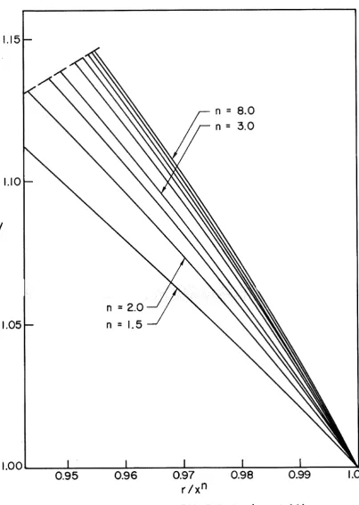
Equation (2.38) with the inftial conditions Eqs. (2.39) was pro- grarmned and integrated numerically on IBM 7094 digital computer, using a fourth order Runge-Kutta method. The sblutims of P(Q, V ( v and

value of y is fixed at 1.40 while the values of n ranges from 1 to 10.

As the results presented in Fig. 2 shows, the flow field at n = 10 al-

ready approaches that of the exponential flow field (see Ref. 7) which

is a limiting case of the power-law flow field; it does not seem nec-

essary to go beyond n = 10.

Except for the case n = 1, the point

7

= 0 is a singularity of the differential equation and therefore integration can only be continued

to a point close to

7/

-

0 . The step size ~TJused in the integration

is usually 1 8 at the beginning and reduced to 2?10-~ for

71

r 5 ~ 1 0 - ~ . Values of G(Q, Gr(n), P(V, V ( v and R(Q are obtained for each value

of

7.

Since we know from the local behavior analysis made in previous

I

section that

as 7) 0, the numerical integration is stopped at some small positive

$

where G*(Q is satisfactorily described by Eq. (2.55). More ex-

plicitly, the computation stops at 'll =

%

when the neighboring points

of

$,

called

%

1

'

,

R3,

etc. have the property that the ratios (m-1) lny

G'($~) 9

G'~%~)I%~

'n-l)'ny and

G'(%,)/&~

b-1) Iny ate

approximately equal to four significant digits. Values sf

n,

-4

found in the present investigation are usually sf the order of PO

.

Therefore, t h e body shape f a c t o r b i s found t o be

Also t h e s u r f a c e value of P(@ can be obtained froan E q e (2,40b) a s

l y - l

p(0) =

(-i

+

l)Y

(clblY

where C1 i s t h e constant obtained from t h e r a t i o s G ' ( & ) f & (m- uf ny

1 B

etc..

,

and Eqs , (2.55) and (2.58) Rave been used. The s u r f a c e value of

V(@

%a simply

F i n a l l y , Eg. (2.56) should be used t o describe t h e d e n s i t y f i e l d near t h e s u r f a c e with C p determined i n a way s i m i l a r t o CIS and of course,

R(o) = ( f o r n

>

1) (2.61)

Pt i s noted h e r e t h a t f o r a f i x e d set of values ( n 3 y ) , t h e values of P, V and @ a r e p r a c t i c a l l y constant t o no l e s s than four decimal

-

3

p l a c e s h e n

7

f a l l s below 10

.

Therefore, f o r our purpose, t h e accu- r a c y of the equations f o r s u r f a c e v a l u e s derived above i s more than s u f f i c i e n t .

conversion, but the accuracy of the results is believed to be unaffected due to the small step size used in the calculation. In the following chapters, the ~hysicist's notation will be used, i.e., we shall write

p ( r D

= P(G) etc.

111.' Geometrical and Aerodynamic P r o p e r t i e s of t h e L i f t i n g Surface.

3.1 General Considerations.

A l i f t i n g s u r f a c e i s defined h e r e a s a stream s u r f a c e , one s i d e of which i s uqed a s t h e compression s i d e of an a c t u a l ying. The l i f t - i n g s u r f a c e copsidered i n t h i s t h e s i s i s t h e stream s u r f a c e generated by a s h e e t of streamlines which o r i g i n a t e from a cum; drawn on t h e

*

*n

s l e n d e r axisyrmnetric shock s u r f a c e of t h e form r = TX considered

i n Chapter 2. This curve i s c a l l e d t h e leading edge of t h e l i f t i n g

, surface. The segment of t h e b a s i c shock wave downstream of t h e lead-

i n g edge w i l l t h e r e f o r e be a t t a c h e d t o t h e l i f t i n g s u r f a c e a l l along i t s leading edge. I n t h e region bounded by t h i s segment of t h e b a s i c shock wave and t h e l i f t i n g surface, t h e o r i g i n a l flow f i e l d w i l l re-

g~ *n

main unchanged when t h e o r i g i n a l axisymmetric power-Paw body r = ~ b x i s replaced by such a l i f t t n g s u r f a c e , g e n e r a l l y t h r e e dimensional, Therefore, t h e flow f i e l d i s known i n t h i s region and t h e f o r c e s a c t - i n g on t h a t s i d e of t h e l i f t i n g s u r f a c e which f a c e s the a t t a c h e d shock wave can be c a l c u l a t e d using t h e s o l u t i o n s of t h e b a s i c flow f i e l d . It i s t h i s shock-facing s i d e of t h e s u r f a c e t h a t w i l l be used a s t h e lower s u r f a c e of an a c t u a l wing. The c a l c u l a t i o n i s exact with r e - gard t o t h e HSDT equations, although i t i s s t i l l asymptotic a s f a r a s t h e complete gasdynamic equations a r e concerned.

azimuthal angle.

A

related rectangular cartesian coordinate system

(x,y,z) with its origin fixed at the nose of the basic shock wave will

also be used for auxiliary purpose, The relation of the two system is

given as follows (see Fig. 1):

and

3

xr =

c

sin (j 9

3

cos qi

;f$ =

C

cos (j

-

j)

sin qi

4 4 4

where

(zx9?r,l

) and (i,j,k) denote two sets of unit vectors associated

f$

with the cylindrical system and the eartesian system respectively. It

should be recalled here that both systems refer to the so-called hyper-

sonic coordinates in the sense that the lateral coordinates y,z in the

eartesian system and r in the cylindrical system have been stretched by

T in accordance with the HSDT analysis.

The lifting surfaces investigated in the present thesis have these

x = 1 (henceforth r e f e r r e d t o a s t h e t r a i l i n g edge plane) and j o i n s t h e leading edge which l i e s on t h e b a s i c shock wave a t two p o i n t s on t h e shock surface. Thus tlie closed curve formed by t h e s e edges i s t h e boundary l i n e s f t h e surface; (3) t h e azimuthal dimension of t h e s u r f a c e i s such t h a t

($11

s

4;

and (4) no expansion region e x i s t s on t h e shock f a c i n g s i d e of t h e l i f t i n g surface. Property (2) a b w e i s s u f f i c i e n t t o a s s u r e a supersonic t r a i l i n g edge s o t h a t t h e flow f i e l d upstream of t h e t r a i l i n g edge w i l l not be influenced by any downstream conditions; i t a f s s s i m p l i f i e s t h e c a l c u l a t i o n s s i g n i f i c a n t l y . Prop- e r t y (4) is introduced t o make s u r e t h a t t h e caPculation of t h e aero- dynamic f o r c e s is indeed made on t h e high pressure s i d e of t h e surface.

3,2 The ~ x ~ r e s s i o n of t h e Stream Function.

I n t h i s s e c t i o n , an a n a l y t i c expression of t h e stream function 'fr

i s derived f o r t h e axisgnrmnetric flow f i e l d considered in Chapter 2. This f o m s t h e b a s i s sf t h e geometrical aspect of t h e problem and i s consequently e s s e n t t a l t o t h e c a l c u l a t i o n of t h e aerodynamic f o r c e s m t h e P i f t f n g surface.

Recall from Eq. (2.33) t h a t a stream function y(x,r) was defined a s s a t i s f y i n g t h e c o n t i n u i t y e q u a t i m i d e n t i c a l l y , i.e.,

Next we introduce t h e s i m i l a r i t y p r o p e r t i e s of t h e flow.

I f we follow t h e P h y s i c i s t ' s convention and w r i t e y(x,r) = y(x,G) e t c . , then m transforming t h e independent v a r i a b l e s f r m (x,r) i n t o

Also, using the similarity properties of the functions a9v, we have

Therefore, Eqs, (2,33) become

--

I

a

Y(X,G) = X~GR(G)

n i3G (3.44

X

To solve the system (3.4) for Y(x,G), Eq. (3.4a) is first smbsti- tuted into (3.4b) to yield

which Pa immediately integrated along a similarity Pine @ = constant to give

Differentiating Eq. (3.5) with respect to G and using Eq. (3.4a),

we have an equation for F(G) as

x2" [ 6 2 g t

-

2-

(RV

+

GR'V

+

GRV')]

.

F?(D) =

-

2

Y + X

The original continuity equation (2.17a.f in (x,@) coordinates takes

the form

after using the similarity representation (3.3) for o and v,

Thus F'(G) = 8 and F(G) = const = 0 so that y(o,G) = 8. Finally,

the analytic representation of y is obtained as

and a streamlPne in this flow field is represented by

3,3. Geometry of the Lifting Surface.

Pt seems convenient for the purpose of discussion to divide the

lifting surfaces into two types;

(A)

the surface contains a portion of

The l i f t i n g s u r f a c e can be determined e i t h e r by p r e s c r i b i n g i t s leading edge shape on t h e b a s i c shock wave o r by p r e s c r i b i n g i t s t r a i l - i n g edge shape i n t h e plane x = 1. These two methods w i l l be discussed i n t h e following.

3.3.1. L i f t i n g Surface With Prescribed Leading Edge.

Suppose t h a t t h e leading edge i s prescribed on t h e shock s u r f a c e a s

s o t h a t i t i s symmetric with r e s p e c t t o qj = 0. The condition L(xO) = 0

f o r xo

>

O i s imposed on t h e function i(x) t o assure t h e c o n t i n u i t y of t h e leading edge curve a t x = x _o Rowever L(o) = O i s not necessary be-

e

cause x = o r e p r e s e n t s only a point on t h e shock s u r f a c e , P e e . , t h e nose, hence c o n t i n u i t y i s tmplied i f t h e leading edge goes through t h e nose. The s i g n i f i c a n c e of t h e nom-negative constan$ x i s t h a t i t serves t o

8

d i s t i n g u i s h type A s u r f a c e (xo = o) from type B surface (xo

>

0). This w i l l be discussed l a t e r i n t h i s sectlon.

The streamline t h a t p e n e t r a t e s t h e shock wave a t t h e point (x,r,@) =

[+.

g9

I ( % ) ] on t h e leading edge has t h e following parametric repre-

Equation (3.10a) can be solved explicitly for

s,

using Rs = Vs = 1,

to give

Combining Eq. (3.11) with Eq. (3,10b), we get an analytic expres-

sion for the lifting surface:

Is]

= L < s >

(3.12)

with xo r s(x,r) =

The trailing edge of this surface is the intersection of this sur-

face and the plane x = 1 and is hence easily found to have the follow- ing representation:

I

+

1 1 %2n

with xo r r*(r) = Y-- rR(r)

The boundary line of the lifting surface has thus been determined

and some of its normal projections will be deduced below:

Projection onto the Trailing Edge Plane:

Elimination of x from Eq. (3.10) gives the leading edge projection:

Obviously, the trailing edge has its true shape in this plane.

Projection onto the Plane y = o: (Planform)

Elimination of y from Eq. (3 .lo) and conversion into the cartesian

?

coordinates (using Eq, (3.1)) give the leading edge projection in terms of cartesizm coordinates,

1 /2

121 = (x2"

-

z2) tan [ ~ ( x )

1

or equivalently'

n

121 = x sin [L(x)]

.

(3.15)

The trailing edge is projected as a segment of x = 1 in the x-z

plane.

Projection onto the Plane z = o: (Elevation)

Elimination of z from Eq. (3.10) and conversion into the cartesian

coordinates give the leading edge projection:

or equivalently

n

y = x cos [L(x)]

.

(3.16)

Again, the trailing edge projection: is simply a segment of the

straight line x = 1.

The equation of the center line of the lifting surface can also be

*

obtained. Due to the assumed symmetry of the surface, this line is simply

the streamline lying in the plane @ = s and originating from the point (x,r,@) = (s,$;n!~(x,J) on the leading edge with I..(+) = o. Its equa-

tion hn the plane $ = o ( z = o) is implicitly given as [see Eq. (3.12)]

because y = a: in the plane (b = 8 . A more convenient expression will be

der5ved later in am example where an explicit form of L(x) is given. It is noted here that the shapes of trailing edge and the center

Pine serve to give some feeling of the transverse and fangitudinal cur-

vature respectively of the lifting surface,

Finally, it will be shown that the case xo = O corresponds to type

A. surface whereas the case xo

>

0 corresponds to type B surface. This

is done with a study of the equation bf the trailing edge (3.13). First, it is observed that the parameter r*(r) defined in Eq. (3.13)

has the property that r*(l) = f and r*(b) = 8 and is monotone in O I; r 5 1

/

can e a s i l y be shown by u s i n g t h e shock wave c o n d i t i o n s on V and R.

That r*(b) = 0 i s obvious f o r t h e c a s e n S 1 where i t h a s been shown 2

t h a t R(b) = 0 o r f i n i t e and a l s o [r

-

~ ( r ) ] = 0 a t r = b due t o t h e body s u r f a c e c o n d i t i o n of t h e o r i g i n a l b a s i c flow. For n 7 1, it

h a s been e s t a b l i s h e d (see s e c t i o n 2.2) t h a t R

-

C 2 T

-

(n-1) lny [Eq. (2.5 6)

1,

2

V

-

r

-

2 v 1 q (n-1) l n y

Y + l [Eqs. (2.40) and (2.55)l a s

7\

-, 0 , hence

**

-

-

0 a s

1

-

0. Now c o n s i d e r

Case (i): xo

>

0: I n t h i s c a s e r*(r) w i l l not go t o zero. There-

- - - --

f o r e i n t h e plane x = 1, t h e t r a i l i n g edge d e f i n e d by Eq. (3.13) w i l l be such t h a t P > b throughout. Consequently no p o i n t on t h e body s u r -

f a c e ( r = b) e x i s t s i n t h e t r a i l i n g edge. Since n e i t h e r t h e l e a d i n g

edge n o r t h e t r a i l i n g edge c o n t a i n s any p o i n t on t h e s u r f a c e of t h e

b a s i c body, t h e l i f t i n g s u r f a c e must have no p o r t i o n i n common w i t h

t h e b a s i c body s u r f a c e . T h i s conclusion i s a c t u a l l y obvious from physi- c a l c o n s i d e r a t i o n s . Note t l i a t Eq. (3.13) r e p r e s e n t s t h e complete t r a i l -

i n g edge i n t h i s , c a s e , t h e two branches j o i n continuornsly a t a p o i n t

( r , @ = (ro.O) where r0 i s d e f i n e d a s r*(ro) = xo.

Case ( i f ) : x = 0: I n t h i s c a s e r*(r) w i l l range from z e r o t o

0

one, hence t h e t r a i l i n g edge does i n t e r s e c t w i t h t h e c i r c l e r = b ( t h e b a s i c body s u r f a c e ) , A t t h e p o i n t of i n t e r s e c t i o n

I @ $

t a k e s ow t h e v a l u e L(o) which i s n o t n e c e s s a r i l y zero. Let L(o) = Bb. Thus t h e

two branches of t h e curve given by Eq. (3.13) end on t h e c i r c l e r = b

at: t h e p o i n t s (b,@ ) and ( b , - ~ ~ ) r e s p e c t i v e l y , and t h e y mark t h e t r a c e b

I

t h e two branches of t h e leading edge. The complete t r a i l i n g edge must

c o n s i s t of a c i r c u l a r a r c : r = b, -@b s @ S gb i n a d d i t i o n t o t h e curves given by Eq. (3.13). This segment of t h e c i r c l e r e p r e s e n t s a segment of

n

t h e b a s i c power-law body s u r f a c e r = bx

,

"wet" by t h e streamlines o r i g i - n a t i n g from t h e nose (x = 0 ) . It can f u r t h e r be shown t h a t t h e a r e a of

t h i s segment of t h e b a s i c body s u r f a c e (measured by i n c r e a s e s with

i n c r e a s i n g value of L(o) which i s t h e angle extended by t h e two branches of leading edge a t x = o. I f L(o) = o, we have gb = o and t h i s p a r t of t h e s u r f a c e degenerates t o a l i n e , i.e., @ = 0 , r = bxn.

An example: L e t t h e leading edge be prescribed a s

The leading edge has constant e l e v a t i o n y = C > 18.

The e g u a t i m of t h e l i f t i n g surface i s then [see Eq. (3.12)]

The t r a i l i n g edge i s described by [see Eq. (3.13)

1

-1 C

($1

= COS

-

n

=*

1 /2n

with C.'ln S r = rR(r)

[r

-

V ( r j 5 1 9

o r simply

0

h e r e ro i s defined by _{r R(r,)}

me

glanfonn i s [Eq. (3.15)

1

112

l z / = xn s i n C O S -n ~ ~ =(x2"

-

2')

_{(3 .28)} X

bounded by x = 1,

The p r o j e c t i o n i n t h e plane z = 0 takes t h e f o m [E¶. (3.16)

1

a s expected,

The boundary l i n e of t h e s u r f a c e when projected onto t h e t r a i l i n g

edge plane becomes t h e closed c u w e bounded by t h e t r a i l i n g edge curve

The center line of the lifting surface is [~q. (3.17)

1

-

1

cos C = 0

In view of the fact that functions R,V are tabulated as functions the practical computation of the above equation can be facil-

itated by using the following parametric representatPon

Finally, it is obvious that in this example, xO =

c""

>

0 and hence the lifting surface belongs to type B.

3.3.2. Lifting Surface With Prescribed Trailing Edge,

k t the trailing edge of the lifting surface be prescribed in the

where the function @(r) is defined as follows:

Type A: P(r) defined for re11 ,b] with P(b)

=

Gb

> 0 (3,22a)

Type B: P(r) defined for rc[l ,ro] with ro > b and @(ro) = 0

.

(3.22b)

Of course, for type A surface, the trailing edge is completed by a cir-

cular arc r = b between @ =

-

Gb and @ = @b

In this sectiono the geometry of the lifting surface will be dis-

cussed in terms of the trailing edge function @(r) in general. How- ever, it is understood that the surface referred to in the following is

the whole lifting surface excluding that portion which is in common with the basic power-law body r = . bxn, in the case of Type A surface, i.e.,

in the case @(b) > 8 ,

Consider a streamline that leaves the trailing edge plane at a

point on the trailing edge, (x,r,@)

=

[l,F,&P(F)

1.

Its equation is, ac-

cording to Eq. (3.8)

Considering

F

as a parameter and letting it vary from one to r (or b), o

we have E ¶ e (3,213) as a parametric representation sf the lifting surface,

The leading edge is the trace sf the lifting surface on the basic

n

Realizing t h a t

%,

R($) and V ( d on r = x a l l take on t h e value

X

of u n i t y , we r e w r i t e t h e above equation i n a form wh;Cch r e p r e s e n t s a parametrized cqyve on t h e shock s u r f a c e r = xn:

Now t h a t t h e geometry of t h e s u r f a c e and i t s boundary l i n e i s com- p l e t e d , a few p r o j e c t i o n s w i l l be given below:

P r o j e c t i o n i n t h e t r a i l i n g edge plane (x = 1 ) :

Elimination of x from Eq. (3,241 gives t h e leading edge p r o j e c t i o n a s

The t r a i l i n g edge has i t s t r u e shape i n t h i s plane. P r o j e c t i o n i n t h e plane y = o (planfonn)

(

l z (

= xn sin

m

(

3

,

The trailing edge projects as x = 1 in this plane.

Projection in the plane z = o (Elevation)

Elimination of z from Eq. (3.24) gives the leading edge projection as

m

(

y = x cos

~(2)

,

Again the trailing edge projection is x =

P

in this plane,

The equation sf the center Pine of the lifting surface is obviously

given by

for the type

A

surface, and according to Eq. (3.231,

with ro defined by l(ro) = 0

An Example: Let the trailing edge be prescribed as

t

x = l

r c s s @ = % c b f o r b s r r l

r = b

where kprk2 are constants so that the trailing edge is at constant ele- vatgon y = kl (or k2)' Evidently case (i) corresponds to type B surface and case (ii) to type

A

surface. For the purpose of illustration, only

case (i) will be considered below. We have

2 2

2

(>)[$

-

,

$41

= i

.(a

[i

-

-

.(a]

y + l

(3.29) k

-1 1

@ = cos

-

.

P

The leading edge representation is also parametrized as rsee Eq. (3.24)]

The projection of the boundary Pine me0 the trailing edge plane

is

a

closed c u w e represented by

k -1 1

= eos

-

r"

and the real trailing edge.

The plaaf o m is [see Eq. (3 2 6 ) ]

-47-

The projection of the boundary line in the plane z = o is

also joined by the segment of the straight line x = 1.

The equatip of the center line of the surface is [see Eq. (3.28)j

The analytical discussion of the geometry of the lifting surface

presented abwe should be sufficient to illustrate the geometrical as-

pect of the surface, Further Snfomation can be obtained by properly

using the equations derfved abwe. It is seen that in a given basic flaw field, Bee., for a given set of values of n and y, a lifting sur- face is determined by specifying either the leading edge shape on the

basic shock surface r = xn or the trailing edge in the plane x = 1,

Graphical construction of the actual three dimensional surface can be

dome with the aid sf the tabulated results of the flow field, using

3.4. Aerodynamic Forces on the Lifting Surface,

In this section, methods of evaluating the lift and drag forces

on the shock-facing side of the lifting surface will be given. First

a direct method is discussed. An indirect method is presented next by

constructing a control volume. The results of this indirect method

will be s h m to be accessible to actual calculation. Original physi-

cal coordinates and flow variables are used in deriving the formulae

and B D T expans+ons introduced in Chapter 2 are used afterwards to

get the leading terms. The order of magnitude sf the error terms will

thus become evident in the process.

3.4.1. Direct Method.

*

Let the lifting surface be denoted by Q

.

Then the pressure force

acting on the shock-facing side of it is the following integral w e r

the lifting surface.

-D

where n is the unit normal of the lifting surface directed away from the

* *

*

side on which the pressure acts, If we denote by L

,

D and T the lift

-0 9

force (acting in (- J) direction), the drag force (acting Pn L direction) -?

and the side thrust (acting in

k

direction), then w e have

*

*

, * = J

J P ds*

*

*

i n which ds

*

i s the normal projection of d s onto the plan, i . e . , Y

*

and

*

_{i s consequently t h e planform of t h e l i f t i n g surface, ds}

*,

*

3 _X

0

*

and ds

*,

n

a r e s i m i l a r l y defined,

X z z

Wow, i n t h e WSDT l i m i t ,

ak

ds

*

= ~ d x d z e t c .

3

z\ Y

Therefore, t h e l i f t f o r c e , f o r example, can be expressed a s

Here g i s a known function, i . e . ,

but In order t o c a l c u l a t e t h e leading term of E, the function P

-

t n ) must be expressed a s a function of ( x , ~ ) , using t h e equation of the

l i f t i n g surface

2 2lI2

to eliminate r = (y

+

z ) in favor of (x,z) and then carry out the in-

tegration over the planform.

As shown in the previous section, the function B(x,r,@) is very t

implicit, hence the process of eliminating r from P

tn)

-

would be ex-

tremely laborious. Therefore, the direct method is inconvenient for

practical purpose, although it is applicable in principle.

I

3.4.2. Indirect Method,

*

Consider a fixed control volume bounded by a closed surface

c

in

a flow field discussed in Chapter 2. Application of the laws sf con-

servation sf mass and momentum to the fluid inside this volume gives

the following equations:

if the effect ~f body force is neglected,

Generalizing Woods' (5' idea, we choose a control volume with its bounding surface formed by these elements: (see Fig. 5)

*

(1)

n

: the lifting surface

*

(2) sl: in plane x = 1, bounded by a segment of the trace of the basic shock wave and the kmplete trailing edge of the

*

*

*

( 3 ) s

+

s3: s is the normal pojection of the lifting surface

2 2

*

onto the plane x =

xo,

which is perpendicular to the

undisturbed streamlines and passing through the apex of

*

*

the lifting surface; s3 is+the normal projection of s 1

*

onto the plane x = xo and is thus its true shape.

*

( 4 ) S 4 : A surface formed by the sheet of undisturbed streamlines

*

*

which connect the boundary line of s2 9 s with the lead- 3

*

Png edge and the upper boundary of s g , which is a segment

of the trace of the basic shock wave in the trailing edge

plane,

*

W%th elements of C so chosen, we have the fo1Powing results:

*

+*

-b 9

On 0 : q a n = 0 , n = m i t normal vector directed toward the

pressure-acting side.

*

*

*

+*

" -P 4

(s2 + s3): P = 3.P

P

' Pa. (1 = k i i OD 9 n = - i

The last term in Eq. (3.37) is the pressure force exerted on the

lifting surface by the fluid. We write

*

as in section 3.4.1 and remark again that the lift force L is taken

+

in the negative j direction. Also, we consider p, = 0, Then Eq. (3.37)

becomes

after Eg. (3.36) has been used.

Notice from above that the aerodynamic forces are expressible in

terms sf integrals in the trailing edge plane,

Introducing the limiting HSDT expansions sf Chapter 2 [ ~ q . (2.6) ]

+

-b

Using thd relation

4

= k sin $

+

f

cos q5, we obtain the following

-

5

L* = T3

JJ

gY cos

g

rdrd$

+

~ ( r

2 f'

,Uco s

I!

7

5

T*

= T~

JJ

sin $ r d r d g + O ( T )

.

I?

(3.40)

Pa0 eo s

P

The quantity u in Eqo (3.38) can be eliminated by using Eq. (2.12) to give

Thus, i n s1 where x = 1 t h e q u a n t i t i e s v,p,o a r e a l l functions of

r alone and i f we write

then we get

2% =

-

n

fl

R(r) V(r) cos ) rdrd$ Y

-

"1

2T =

-

n

JJ

R(r) Y ( r ) s i n (b rdrd@

Y

-

1

Note t h a t (2D), (2E) and (2T) a r e t h e leading terms of t h e dimen- sisnPess drag, l i f t and s i d e t h r u s t r e s p e c t i v e l y and t h a t they a r e a11

bounded by the trailing edge curve and a segment of the basic shock

wave and is hence symmetric with respect to @ = o. If we first inte-

grate along r = const. from @ =

-

@(r) to @ =

+

@(r) then the follow-

ing results are obtained:

2

I =

-

n RV sin $(r) rdr Y - 1

where ) @ $ = i ( r ) is the trailing edge equation hi&, in the case of

type

A

surface, does not include the circular arc P = b, Also,

r = r

z

b with @(ro) = o for a type B surface and r = b for a type

a 0 a

A surfacee

In order to facilitate writing, the following notations are intro- duced

(r;m,y) = drag function = n2(~$+p)r (3.44) y2

-

1

&

(r;m,y) = lift function = (3.45)

so that

I, = r ~ ( r ) s i n g(r)dr.

It i s seen t h a t t h e c a l c u l a t i o n of D and L involves only s i n g l e i n t e g r a t i o n s . Functions a ( r ; n ,y) and x ( r ; n ,y) a r e f i x e d functions of r f o r every given flow f i e l d and thus can be c a l c u l a t e d once f o r

a l l with given n and y, using t a b l e 1, Once @ ( r ) i s s p e c i f i e d , t h e e v a l u a t i o n of D and E i s s o simple t h a t even hand c a l c u l a t i o n i s p r a c t i - caP. The advantage of t h i s method over t h e p r e v i m s one i s thus e v i -

dent.

It might appear t h a t a d i f f i c u l t y e x i s t s f o r a type A surface with n > 1 because we have then ra = b a n d , 8 ( b ) = w. However i t w i l l be

shown below t h a t t h i s s i n g u l a r i t y i s an i n t e g r a b l e

me.

Consider t h e c o n t r i b u t i o n t o t h e l i f t from t h e elements between r = r and r = b

a

where r i s s l i g h t l y g r e a t e r than b, and denote t h i s l o c a l contribu-

a

t i o n b y E Then,

a'

r

R

=

x(r)

s%n $ ( r ) d r =

-

dG

5

Y O 1 2n P C ( @ R('@ V(@

q

s i n

0 7

where

7

i s defined a s @(q ) = r and again t h e ~ f i y s i c i s t ' s convention

R

a

a

R(G) = HI(@ e t c , has been used,

According t o t h e a n a l y s i s of t h e f o c a l behavior of t h e functions R,V,@,@* i n s e c t i o n 2.2, we have