Method of fragments (MoF) solutions for double-walled, circular and rectangular cofferdam seepage problems

This file is part of the following work:

Madanayaka, Thushara Asela (2018) Method of fragments (MoF) solutions for

double-walled, circular and rectangular cofferdam seepage problems. PhD Thesis,

James Cook University.

Access to this file is available from:

https://doi.org/10.25903/5c99693025545

Copyright © 2018 Thushara Asela Madanayaka

The author has certified to JCU that they have made a reasonable effort to gain

permission and acknowledge the owners of any third party copyright material

included in this document. If you believe that this is not the case, please email

double-walled, circular and rectangular cofferdam

seepage problems

By

Thushara Asela Madanayaka BSc (Eng) Hons, M.Eng.

This thesis submitted for the

Degree of Doctor of Philosophy

(Geotechnical Engineering)

College of Science and Engineering

James Cook University

ii I, the undersigned, the author of this thesis, understand that James Cook University will make it available for use within the University Library and, by microfilm or other means, allow access to users in other approved libraries.

All users consulting this thesis will have to sign the following statement:

In consulting this thesis, I agree not to copy or closely paraphrase it in whole or in part without the written consent of the author; and to make proper public written acknowledgement for any assistance which I have obtained from it.

Beyond this, I do not wish to place any restriction on access to this thesis.

………. ……….

iii DECLARATION

I declare that this thesis is my own work and has not been submitted in any form of another degree or diploma at any university or other institution of tertiary education. Information derived from the published or unpublished work of others has been acknowledged in the text and a list of references is given.

………. ……….

Signature Date

DECLARATION – ELECTRONIC COPY

I, the undersigned, the author of this work, declare that to the best of my knowledge, the electronic copy of this thesis submitted to the library at James Cook University is an accurate copy of the printed thesis submitted.

………. ……….

iv

Grants : This research work was supported by the scholarship (JCU PRS) and

research grants (to participate international conferences) of Graduate Research School of James Cook University (JCU), and also, Doctoral Completion Grant provided by the College of Science and Engineering of JCU.

Supervision : A/Prof. Nagaratnam Sivakugan was the primary supervisor (JCU) for

this Ph.D. and the additional supervision was provided by Dr. Peter To (JCU).

v Firstly, I would like to express my sincere gratitude to my primary supervisor Prof. Nagaratnam Sivakugan for the continuous advice and support of my Ph.D., for his patience, motivation, and immense knowledge. His invaluable guidance helped me in all the time of research and writing of this thesis. Thank you, Prof. Siva, without your untiring efforts and guidance, my Ph.D. research would not have been a success.

Besides my primary supervisor, I would like to thank my secondary supervisor Dr. Peter To for his insightful comments and encouragement. Also, my sincere thank is to Dr. Jay Ameratunga (Principal Geotechnical Engineer at Golder Associates) for his kind advises.

My sincere thanks also go to Mr. Warren O’Donnell (Former geomechanics laboratory manager) and current laboratory managers Mr. Shaun Robinson and Mr. Troy Poole for providing laboratory and research facilities and for their guidance. I thank my university colleagues and all the staff of College of Science and Engineering for their constant support. In particular, I am grateful to Mrs. Norton Melissa for her priceless assistance.

In addition, I wish to acknowledge the Graduate Research School (GRS) providing me the scholarship, the living stipend, and GRS grants (for international conference participations) during my candidature. Also, my sincere gratitude to College of Science and Engineering for providing financial support (Student Support Allocation) and Doctoral Completion Grant.

vii Cofferdams are temporary structures used in construction sites. Long-narrow (double-walled), circular, square and rectangular are the commonly seen cofferdam shapes, and flow rate and maximum exit hydraulic gradient are two of the main design parameters required. Commonly, these are evaluated through the 2D ground water flow model solved using flow nets or numerical methods. However, when the flow pattern is 3D, such as flow into the square or rectangular cofferdams, predictions by the 2D models underestimate the flow rate and maximum exit hydraulic gradient values considerably.

viii cofferdams enabling quicker computations and the MoF be implemented in spreadsheets.

In addition, a simple method for evaluating the cofferdam safety against possible piping failure is presented. Through a series of finite element simulations, simple expressions were developed and validated to estimate the maximum exit hydraulic gradient for both double-walled and circular cofferdams considering only the shortest seepage path, known as creep length. The proposed solutions, including mean, lower and upper bound values for the exit hydraulic gradient at a given creep length can be applied in both isotropic and anisotropic soil conditions. Using them, a first-order estimate of the required creep length to limit the exit hydraulic gradient to a specific value can be determined. Alternatively, for a given configuration of the cofferdam, the exit hydraulic gradient can also be estimated. These equations can be valuable tools for back-of-the-envelope calculations in the preliminary analysis while selecting the dimensions in a cofferdam.

x

Book

1. Madanayaka, T. A., and Sivakugan, N.Confined Flow Through Soils: The Method of

Fragments Approach. CRC Press (draft in progress).

Journal Articles

1. Madanayaka, T. A., and Sivakugan, N. (2016). Approximate equations for the method

of fragment. International Journal of Geotechnical Engineering, 10(3), 297-303.

2. Madanayaka, T. A., and Sivakugan, N. (2017). Adaptation of Method of Fragments to

Axisymmetric Cofferdam Seepage Problem. International Journal of Geomechanics,

ASCE (9), doi: 10.1061/(ASCE)GM.1943-5622.0000955.

3. Madanayaka, T. A., and Sivakugan, N. (2018). Simple solutions for square and rectangular cofferdam seepage problems. Canadian Geotechnical Journal (In print).

4. Madanayaka, T. A., and Sivakugan, N. (2017) “ Validity of the method of fragments

for seepage analysis in circular cofferdams” Geotechnical & Geological Engineering, (Under the second review).

5. Madanayaka, T. A., and Sivakugan, N. “ Relationship between minimum creep length

xi

1. Madanayaka, T., and Sivakugan, N. (2016) Simplified method of fragments based two

dimensional seepage solution for the double-wall cofferdam. Proc., 19th Southeast Asian Geotechnical Conference, 1047-1051, 31 May-03 June 2016, Kuala Lumpur,

Malaysia.

2. Madanayaka, T., Sivakugan, N., Ameratunga J (2017) Validity of the method of

fragments for seepage analysis in double-wall cofferdams. Proc., 19th International

Conference on Soil Mechanics and Geotechnical Engineering, 2921-2924, 18-22,

xii

Statement of Access ii

Statement of Sources iii

Statement of Contribution of Others iv

Acknowledgements v

Abstract vii

List of Publications x

Table of Contents xii

List of Figures xix

List of Tables xxvi

CHAPTER 1 INTRODUCTION 1

1.1 General 1

1.2 Cofferdams 2

1.3 Current State-of-the-Art 6

1.4 Objectives and scope of research 7

1.5 Relevance of the research 8

1.6 Thesis overview 9

CHAPTER 2 LITERATURE REVIEW 12

2.1 Overview 12

2.2 Soil permeability 12

2.2.1 Factors affecting the soil permeability 13

2.2.2 Laboratory determination of soil permeability 14

xiii

2.3 Darcy’ law and range of validity 22

2.3.1 Reynolds number 23

2.3.2 Laboratory study on Reynolds number 25

2.4 Hydraulic failure mechanisms of cofferdams 32

2.4.1 Piping failure mechanism 32

2.4.2 Heaving failure mechanism 33

2.4.3 Critical failure mechanism 34

2.5 Seepage solution methods for cofferdams 35

2.5.1 Seepage solution methods for double-walled cofferdams 36

2.5.2 Seepage solution methods for circular cofferdams 41

2.5.3 Seepage solution methods for square and rectangular cofferdams 44

2.5.4 Design charts 46

2.5.5 Method of fragments (MoF) 47

2.6 Summary and conclusions 52

CHAPTER 3 VALIDITY OF METHOD OF FRAGMENTS (MOF) SOLUTIONS

FOR DOUBLE- WALLED COFFERDAMS 53

3.1 Introduction 53

3.2 Method of fragments (MoF) solutions for double-walled cofferdams 53

3.2.1 Flow rate q estimation 55

3.2.2 Exit hydraulic gradient 𝑖_𝐸 estimation 56

3.3 Accuracy of MoF solutions for double-walled cofferdams 56

3.3.1 Numerical modeling of double-walled cofferdams 57

xiv

3.3.4 Effects of assumption deviation on the seepage solutions 63

3.4 Expressions for form factors and exit gradient estimations 66

3.4.1 Expressions for fragment type C 66

3.4.2 Expression for fragment type A 71

3.4.3 Validation of proposed form factors and exit hydraulic gradient expressions 73

3.5 Summary and conclusions 73

CHAPTER 4 METHOD OF FRAGMENTS (MOF) SOLUTIONS FOR CIRCULAR

COFFERDAM SEEPAGE PROBLEMS 76

4.1 Introduction 76

4.2 Numerical simulation of circular cofferdams 76

4.2.1 Axisymmetric numerical model validation 77

4.3 Flow net solutions for circular cofferdams 81

4.4 Adaptability of method of fragments (MoF) solutions for circular cofferdams 85

4.4.1 Validity assessment of the assumption for equipotential line behaviour 86

4.5 Development of method of fragments (MoF) for circular cofferdams 88

4.5.1 Development of design charts required for axisymmetric MoF solution 89

4.6 Validation of MoF solutions for circular cofferdams 94

4.6.1 Comparison against finite element solutions 95

4.6.2 Comparison against analytical solutions 97

4.6.3 Comparison against experimental results 100

4.7 Development of expressions for axisymmetric form factors and exit hydraulic

gradient estimations 112

xv

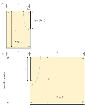
4.7.3 Fragment D normalised exit hydraulic gradient 114

4.7.4 Validation of the proposed expressions 115

4.8 Summary and conclusions 116

CHAPTER 5 RELATIONSHIP BETWEEN MINIMUM CREEP LENGTH AND MAXIMUM EXIT HYDRAULIC GRADIENT IN

DOUBLE-WALLED AND CIRCULAR COFFERDAMS 119

5.1 Introduction 119

5.2 Factor of safety applied against piping failure 119

5.3 Line of creep method 120

5.4 Line of creep method for double-walled cofferdams 123

5.4.1 Relationship between creep length and maximum exit hydraulic gradient

of double-walled cofferdams 124

5.4.2 Upper and lower bound curves for double-walled cofferdams 128

5.4.3 Validation of the proposed solutions for double-walled cofferdams 132

5.5 Line of creep method for circular cofferdams 134

5.5.1 Relationship between creep length and maximum exit hydraulic gradient 135 of circular cofferdams

5.5.2 Boundary curves for circular cofferdams 138

5.5.3 Validation of the proposed solutions for circular cofferdams 139

5.6 Approximate creep ratios for cofferdams 140

xvi

COFFERDAM SEEPAGE PROBLEMS 145

6.1 Introduction 145

6.2 Seepage solutions for square cofferdams 145

6.2.1 Numerical simulations of square cofferdams 146

6.2.2 Accuracy assessment of current approximate seepage solution methods for

square cofferdams 152

6.2.3 Proposed solution method for square cofferdams 160

6.3 Seepage solution for rectangular cofferdams 163

6.3.1 Numerical simulations of rectangular cofferdams 163

6.3.2 Accuracy assessment of double-walled approximation to the seepage

solutions for rectangular cofferdams 165

6.3.3 Proposed solution method for rectangular cofferdams 169

6.4 Summary and conclusions 175

CHAPTER 7 SUMMARY, CONCLUSIONS AND RECOMENDATIONS 177

7.1 Summary 177

7.2 Conclusions 181

7.2.1 Method of Fragments (MoF) solutions for double-walled and circular

cofferdams 181

7.2.2 Creep length solutions for piping failure assessment of double-walled

and circular cofferdams 182

7.2.3 Approximate seepage solutions for square cofferdams 182

xvii

7.3.1 Method of Fragments (MoF) solutions for double-walled cofferdams 184

7.3.2 Method of Fragments (MoF) solutions for circular cofferdams 184

7.3.3 Creep length solutions for piping failure assessment of double-walled

and circular cofferdams 185

7.3.4 Seepage solutions for square and rectangular cofferdams 185

7.4 Final comments 186

REFERENCES 187

APPENDIX A1 Comparison of Griffiths (1984) fragment C form factor

values with the derived values in this desertion 197

APPENDIX A 2 Comparison of Griffiths (1984) fragment C normalised exit

hydraulic gradient values with the derived values in this

desertion 198

APPENDIX A 3 Comparison of Griffiths (1984) fragment A form factor values

with the derived values in this desertion 199

APPENDIX B1 Developed axisymmetric form factor values of fragment D 200

APPENDIX B2 Developed axisymmetric form factor values of fragment E 201

APPENDIX B3 Developed normalised exit gradient values of fragment D 202

APPENDIX B4 Laboratory simulation results of circular cofferdams 203

APPENDIX C1 𝑖_𝐸/ℎ values of double-walled cofferdams 204

APPENDIX C2 𝑖_𝐸/ℎ values of circular cofferdams 206

APPENDIX D1 Relation of double-walled cofferdam flow rate to the rectangular

xviii

cofferdams 209

APPENDIX D3 Relation of double-walled cofferdam 𝑖𝐸 to the 𝑖𝐸𝑆 of rectangular

cofferdams 210

APPENDIX D4 Relation of double-walled cofferdam 𝑖_𝐸 to the 𝑖_𝐸𝐶 of rectangular

xix

Figure Description page

1.1 Cofferdam shapes: (a) long-narrow; (b) circular; (c) square; (d) rectangular 3

1.2 (a) Elevation; (b) plan views (section X-X) of a cofferdam under four possible flow

patterns 5

2.1 Schematic diagram of constant head test set-up [adopted from Das and Sivakugan

(2016)] 15

2.2 Schematic diagram of falling head test set-up [adopted from Das and Sivakugan

(2016)] 16

2.3 Equivalent permeability determination in stratified soil 20

2.4 Grain size distributions for three samples 26

2.5 Permeameter apparatus 27

2.6 Constant head permeability test set-up 28

2.7 Observed Darcy and nonlinear flow behaviours 29

2.8 i-v plots for laminar flow regime 31

2.9 Failure due to heaving in front of a single row of sheet pile (Das 2013) 34

2.10 Experimental model geometry studied by Marsland (1953) 35

2.11 Flow element in two-dimensions 36

2.12 Flow net for the double-walled cofferdam in 2D Cartesian plane (Craig 2004) 38

2.13 Numerical model geometry for double-walled cofferdams 41

2.14 Axisymmetric plane in cylindrical coordinate system for circular cofferdams

Neveu (1972) 42

xx 2.16 Required penetration of cut-off wall against piping or heaving [adopted from U.S.

Department of the Navy (1982)] 47

2.17 Method of fragments for concrete dam 48

3.1 Adoption of MoF for double-walled cofferdams 54

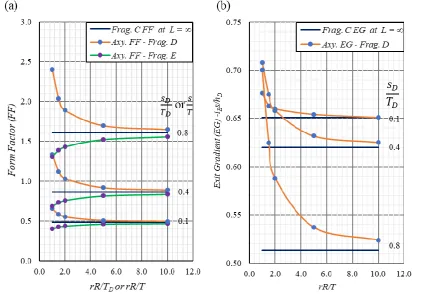
3.2 Form factor charts: (a) fragment A; (b) fragment C [adopted form Griffiths (1984)] 54

3.3 Normalised exit gradient chart for fragment C [adopted form Griffiths (1984)] 55

3.4 Numerical model geometry used for simulating double-walled cofferdams 57

3.5 Initial dewatering condition of double-walled cofferdams for the onshore

excavations 58

3.6 Double-walled cofferdam model validation:

(a) flow rate; (b) exit hydraulic gradient 61

3.7 Behaviour of the equipotential lines with double-walled cofferdam geometry 62

3.8 Comparison of predictions from MoF and full numerical model (Full NM)

solutions when α = 0: (a) seepage quantity; (b) exit hydraulic gradient 64

3.9 Effect of cofferdam geometry on the accuracy of MoF solutions:

(a) seepage quantity; (b) exit hydraulic gradient 65

3.10 Numerical model geometry used for fragment C simulations 67

3.11 Form factor 𝛷_𝐶 values for fragment C (from finite element simulation) 69

3.12 Exit hydraulic gradient values for fragment C (from finite element simulation) 70

3.13 Fragment A geometries: (a) actual geometry; (b) equivalent fragment C geometry

used for numerical simulations 72

3.14 Form factor 𝛷𝐴 values for fragment A at b = 0 (from finite element simulation) 72

3.15 Comparison of proposed expressions solutions with full numerical model (NM)

xxi

4.1 Axisymmetric numerical model geometry used for circular cofferdams 77

4.2 Axisymmetric numerical model validation for flow rate estimation of circular

cofferdams 79

4.3 Axisymmetric model validation for average exit hydraulic gradient 𝑖_{𝐸𝐴𝑣𝑔.}⁄ℎ

estimation of circular cofferdams 80

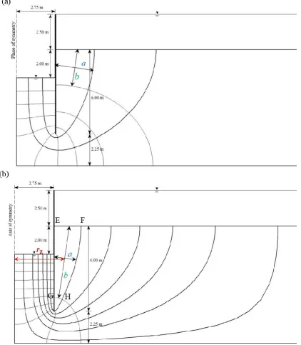
4.4 Circular cofferdam in axisymmetric configuration:

(a) elevation view; (b) plan view 82

4.5 Flow nets: (a) double-walled cofferdam; (b) circular cofferdam 85

4.6 Proposed Axisymmetric fragment types: (a) fragment D; (b) fragment E 86

4.7 Behaviour of the equipotential lines with circular cofferdam geometries 87

4.8 Numerical model geometry used for axisymmetric fragments:

(a) fragment D; (b) fragment E 90

4.9 Convergence of axisymmetric form factor and dimensionless exit hydraulic gradient values to single sheet pile wall values: (a) form factors; (b) exit hydraulic

gradient 91

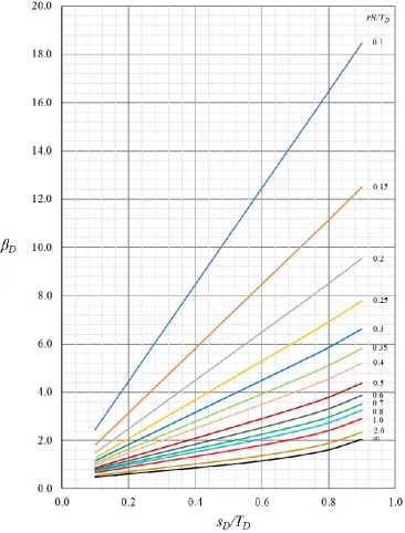
4.10 Form factor 𝛽𝐷 values for fragment D (from finite element simulation) 92

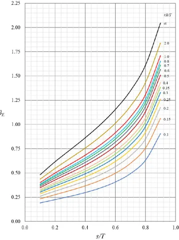
4.11 Form factor 𝛽𝐸 values for fragment E (from finite element simulation) 93

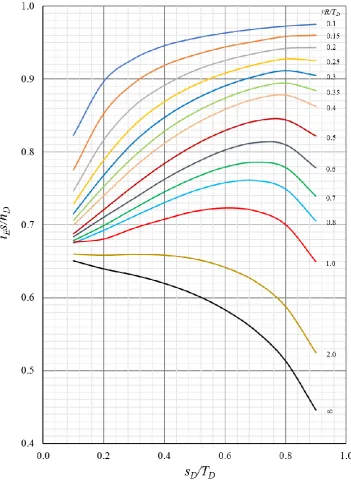
4.12 Exit gradient values for fragment D (from finite element simulation) 94

4.13 Comparison of predictions from axisymmetric MoF and full numerical model

(Full NM) solutions when α = 0: (a) seepage quantity; (b) exit hydraulic gradient 95 4.14 Effect of cofferdam geometry on the accuracy of axisymmetric MoF solutions:

xxii 4.15 Comparison of seepage quantities estimated by proposed axisymmetric MoF

solutions against analytical solutions by Neveu (1972):

(a) α=0; (b) α=0.505; (c) α=0.808 99

4.16 Grain size distributions for three sand samples 100

4.17 Constant head test set-up used for permeability values determination 103

4.18 Relation between permeability and relative density (𝐷𝑟) 104

4.19 a) The schematic diagram of the laboratory test set-up (to scale);

(b) a photograph of the test set-up 105

4.20 Comparison of seepage quantities estimated by proposed axisymmetric MoF

solutions against experimental results 109

4.21 Comparison of seepage quantities estimated by proposed axisymmetric MoF

solutions against experimental results by Davidenkoff and Franke (1965) 111 4.22 Comparison of proposed expressions solutions with full numerical model

(NM) solutions: (a) seepage quantity; (b) exit hydraulic gradient 116

5.1 Line of creep method for a dam problem 121

5.2 Creep length calculation for double-walled cofferdams 124

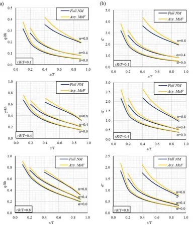
5.3 Changing the normalised 𝑖𝐸 values with cofferdam width in double-walled

cofferdams: (a) 𝑠/𝑇 = 0.2; (b) 𝑠/𝑇 = 0.4; (c) 𝑠/𝑇 = 0.8 126

5.4 Normalised 𝑖_𝐸 vs creep ratio 𝐶_𝑐 relationship for double-walled cofferdams:

(a) 0.1 ≤ 𝐿𝑅/𝑇 < 0.5; (b) 𝐿𝑅/𝑇 ≥ 0.5 127 5.5 Boundary curves for 0.1 ≤ 𝐿𝑅/𝑇 < 0.5:

(a) Upper bound curve; (b) Lower bound curve 129

5.6 Both upper and lower bound curves for normalised 𝑖_𝐸 of double-walled

xxiii

5.7 Validity assessment for double-walled cofferdams:

(a) 0.1 ≤ 𝐿𝑅/𝑇 < 0.5 ;(b) 𝐿𝑅/𝑇 ≥ 0.5 133 5.8 Changing the normalised 𝑖_𝐸 values with cofferdam width in circular cofferdams:

(a) 𝑠/𝑇 = 0.2; (b) 𝑠/𝑇 = 0.4; (c) 𝑠/𝑇 = 0.8 136 5.9 Normalised 𝑖𝐸 vs creep ratio 𝐶𝑐 relationship for circular cofferdams:

(a) 0.1 ≤ 𝑟𝑅/𝑇 < 0.5; (b) 𝑟𝑅/𝑇 ≥ 0.5 137 5.10 Both upper and lower bound curves for normalised 𝑖_𝐸 of circular cofferdams:

(a) 0.1 ≤ 𝑟𝑅/𝑇 < 0.5; (b) 𝑟𝑅/𝑇 ≥ 0.5 138 5.11 Validity assessment for circular cofferdams:

(a) 0.1 ≤ 𝑟𝑅/𝑇 < 0.5; (b) 𝑟𝑅/𝑇 ≥ 0.5 140 5.12 Summary of the equations and curves for the double-walled (DW) and

circular (Cir.) cofferdams: (a) 0.1 ≤ (𝐿𝑅_𝑇 𝑜𝑟 𝑟𝑅_𝑇) < 0.5; (b) (𝐿𝑅_𝑇 𝑜𝑟 𝑟𝑅_𝑇) ≥ 0.5 144

6.1 Numerical model used for square cofferdams: (a) model geometry; (b) 3D mesh 147

6.2 Square cofferdam model validation: (a) flow rate; (b) average exit hydraulic

gradient at middle of a side 𝑖𝐸𝑀𝐴𝑣𝑔.⁄ℎ; (c) average exit hydraulic gradient at

corner 𝑖_{𝐸𝐶𝐴𝑣𝑔.}⁄ℎ 149

6.3 Sensitivity analysis results for square cofferdams: (a) flow rate; (b) exit hydraulic

gradient at mid-point 𝑖𝐸𝑀; (c) exit hydraulic gradient at corner 𝑖𝐸𝐶 151

6.4 Relationships between 2D flow rates (𝑞_𝑐 and 𝑞_𝑑 ) to the 3D flow rate 𝑞_𝑠 into

square cofferdam: (a) axisymmetric flow; (b) Cartesian flow 153

6.5 Deviation of the flow rate predictions of square cofferdam by Eq. 6 and Eq. 8

From the actual flow rate 155

6.6 Double-walled cofferdam geometry and form factors chart used in CFEM (2006)

xxiv 6.7 Relationships between 2D exit hydraulic gradient 𝑖𝐸 values and 𝑖𝐸𝑀 and 𝑖𝐸𝐶

values of square cofferdams: (a) circular cofferdam; (b) double-walled cofferdam 157

6.8 Comparison of the exit gradient predictions using 2D flow patterns: (a) circular

cofferdam; (b) double-walled cofferdam 159

6.9 Comparison of the flow rate predictions for square cofferdams using 2D flow

patterns : (a) circular cofferdam; (b) double-walled cofferdam 161

6.10 Equipotential lines distributions: (a) square cofferdams; (b) circular cofferdams;

(c) double-walled cofferdams 162

6.11 Numerical model geometry used for rectangular cofferdams 165

6.12 Relationship between double-walled flow rate to the 3D flow rate into rectangular

cofferdam at 𝑙/𝐵 = 3 166

6.13 Relationship between double-walled exit gradient to the actual exit gradient values

of rectangular cofferdams at 𝑙/𝐵 = 3 168

6.14 Relationship of a value to the 𝑙/𝐵 ratio 170

6.15 Comparison of the flow rate predictions for rectangular cofferdam at 𝑙/𝐵 = 3 171

6.16 Relationship of b value to the 𝑙/𝐵 ratio on 𝑖𝐸𝐿 estimation 172

6.17 Comparison of the exit hydraulic gradient predictions for rectangular cofferdams:

(a) 𝑖_𝐸𝐶; (b) 𝑖_𝐸𝑆; (c) 𝑖_𝐸𝐿 174

D1.1 Relationship between double-walled flow rate to the 3D flow rate into rectangular

cofferdams 208

D2.1 Relationship between double-walled 𝑖_𝐸 to the actual 𝑖_𝐸𝐿 of rectangular

cofferdams 209

D3.1 Relationship between double-walled 𝑖𝐸 to the actual 𝑖𝐸𝑆 of rectangular

xxv

xxvi

Table Description page

2.1 Typical values of soil permeability in saturated soils

[adopted from (Das and Sivakugan 2016)] 13

2.2 Proposed values for Hazen’s constant c 18

2.3 Empirical relationships for the Forchheimer coefficients of a and b determination

[adopted from (Van Lopik et al. 2017)] 25

2.4 Determined index properties 26

2.5 Summary of the test results 30

2.6 Confined flow fragments and their form factors, Harr (1962, 1977) 50

2.7 Confined flow fragments by Griffiths (1984) 51

3.1 Cofferdam geometries used for numerical model validations 60

3.2 Double-walled cofferdam geometries used for equipotential lines behaviour

Studied 61

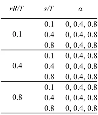
4.1 Cofferdam geometries used for validating the axisymmetric numerical model for

circular cofferdams 78

4.2 Circular cofferdam geometries used for equipotential lines behaviour studied 87

4.3 Cofferdam geometries used for axisymmetric MoF comparisons against analytical

solution by Neveu (1972) 98

4.4 Result of grain size distribution tests 101

4.5 Tests and the list of standards used for determining the physical properties of sand 101

4.6 Physical properties of sand 1 101

4.7 Sequence of the laboratory tests conducted 107

xxvii

4.9 Relative errors between experimental results (using electrical analogy model)

and MoF Predictions 112

5.1 Lane’s recommended values for weighted creep ratio 𝐶_𝑤 123

5.2 Summary of the validity assessment for double-walled cofferdams 134

5.3 Summary of the validity assessment for circular cofferdams 140

5.4 Summary of the estimated creep ratio Cc values for cofferdams 142

6.1 Cofferdam geometries used for validating the 3D numerical model for square

cofferdam 148

6.2 Geometry range used for square cofferdam analysis 153

6.3 Summary of the flow rate analysis of rectangular cofferdam 167

6.4 Summary of the exit gradient estimation relations for rectangular cofferdam 169

A1.1 Griffiths (1984) fragment C form factor 𝛷𝐶 values 197

A1.2 Developed fragment C form factors 𝛷_𝐶 values using finite element simulations 197

A2.1 Griffiths (1984) fragment C normalised exit hydraulic gradient 𝑖_𝐸𝑠_𝐶/ℎ_𝐶 values 198 A2.2 Developed fragment C normalised exit hydraulic gradient 𝑖_𝐸𝑠_𝐶/ℎ_𝐶 values using

finite element simulations 198

A3.1 Griffiths (1984) fragment A form factor 𝛷_𝐴 values when b = 0 199

A3.2 Derived fragment C form factor 𝛷_𝐶 values when 𝐿 = 2𝑇_𝐶 using finite element

simulations 199

B1.1 Developed fragment D form factors 𝛽_𝐷 values using finite element simulations 200

B2.1 Developed fragment E form factors 𝛽_𝐸 values using finite element simulations 201

B3.1 Developed fragment D normalised exit gradient 𝑖_𝐸𝑠_𝐷/ℎ_𝐷 values using finite

element simulations 202

xxviii

1

Chapter 1

Introduction

1.1 General

Excavations are used in construction sites to create foundations for structures such as buildings, bridges, dams etc. When an excavation takes place below the ground water level, it is required to control water seepage into the excavation to provide a dry and safe working environment to the workers within the excavations. Commonly used seepage controlling methods can be identified under three basic groups as follows (Powers 1992):

1. Open pumping: a method that allows water to flow into the excavation and pumps them

away from sumps and ditches.

2. Predrain method: a method that lowers the ground water table before commencing the

excavation using wells, well points or drains.

3. Cut-off method: a method that cuts-off water entering into the excavation using a vertically driven structure.

2

The third one is to apply a water cut-off structure using sheet piling walls, diaphragm walls or grout walls acting as a ground support structure, in addition to reducing the water entering the excavation (Powers 1992). Further, Kavvadas et al. (1992) defined some other unique advantages of water cut-off structures as below:

1. It reduces water seepage into the excavation significantly because of vertically driven structures making barriers to the horizontal flow. This is due to the soil permeability is larger in horizontal direction compared to that in the vertical direction.

2. It lowers the ground water table which is away from the excavation boundary only a

small amount compared to that of the predrain method. So, there is less risk to adjacent structures by settlement induced damages.

3. It decreases the exit hydraulic gradient considerably because vertical structures are driven well below the excavation base, and hence, provides adequate factor of safety with respect to possible hydraulic failure (heaving or piping).

Due to above advantages, water cut-off structures are among the widely used seepage control methods. Water cutoff structures made using sheet piles are usually known as cofferdams and are most suitable for sandy soils and stratified soil systems (Powers 1992). Also, steel is the often seen material for sheet piles for its as high structural strength, driveability, water tightness, reusability and quick construction.

1.2 Cofferdams

3

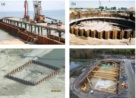
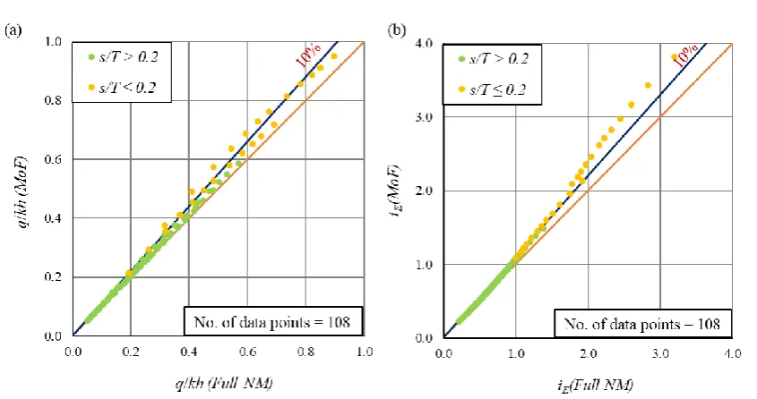
termed as double-walled cofferdams (Harr 1962; Griffiths 1984; Banerjee and Muleshkov 1992; Banerjee 1993), and the same term is used in this thesis also, to define the long-narrow cofferdams. Double-walled cofferdams are commonly used for constructions of foundations for bridge piers, concrete dams and harbour walls (King and Cockroft 1972). For constructions of water treatment plant, sewers, bridge piers, and abutment and shaft, circular cofferdams are employed (Koltuk and Azzam 2016) while square or rectangular cofferdams are encountered with the foundation constructions for buildings, small bridges etc.

4

All the cofferdam shapes discussed above are similar in the cross-sectional elevation view as shown in Fig. 1.2a where the seepage flow is taking place under the total head difference of h. Water seeping into the cofferdam generates the hydraulic gradient, and hence, excavation base failure can occur. Also, presence of a hydraulic gradient affects the stability of sheet pile wall, changing the distribution and magnitude of the water and earth pressure components (Kaiser and Hewitt 1982; Soubra et al. 1999; Benmebarek et al. 2006). Therefore, seepage analysis is a vital factor for designing any shape of cofferdam, and flow rate Q and maximum exit hydraulic gradient 𝑖𝐸 are two important variables that are computed. The flow rate is necessary

to estimate the required pump capacity, maintaining the excavation base dry while exit hydraulic gradient is to assess the stability with respect to possible piping failure. Here, exit hydraulic gradient 𝑖𝐸 is the hydraulic gradient at the excavation base right next to the sheet pile

wall (see Fig. 1.2a) since, exit hydraulic gradient is maximum at that point (Griffiths 1984).

5

6

1.3 Current State-of-the-Art

For double-walled cofferdams, available seepage solution methods are the following: flow net, analytical, numerical, and method of fragments (MoF). Out of these methods, MoF proposed by Griffiths (1984) has a place as a simple and quick method to estimate flow rate and maximum exit hydraulic gradient. Also, it has the ability to incorporate the effect of soil anisotropy, too. However, the accuracy of this method depends on the validity of the assumption that the equipotential lines at tip of the sheet piles are vertical; therefore, the method’s accuracy varies with the cofferdam geometry.

7

Considering all, it can be concluded that, although MoF provides simple and quick seepage solutions for double-walled cofferdam problems, it is still required to assess the effect of violating the assumption (that the equipotential line at the tip of sheet pile is vertical) on the accuracy of the result over a wider range of geometries. Also, it is very useful to have MoF solution method for circular cofferdams. Further, solution methods that can incorporate the effect of 3D flow into the square and rectangular cofferdams will also be more beneficial.

1.4 Objectives and scope of research

The primary goal of this study is to critically assess the adaptability of MoF as a seepage solution method for cofferdams of different geometries, with particular interest on the flow rate and maximum exit hydraulic gradient estimations. Following objectives are established in order to achieve the thesis aim.

1. To assess the effect of violating the assumption that the equipotential line at the tip is vertical on the MoF solutions for double-walled cofferdams.

2. To develop axisymmetric MoF solutions for circular cofferdams which are applicable

to both isotropic and anisotropic soil conditions and validate them over wider range of geometries.

3. To develop and validate a relationship between shortest seepage path (creep length) and maximum exit hydraulic gradient in both double-walled and circular cofferdams in order to use as the first-order approximations in ensuring the safety against piping.

4. To develop and validate a simple and more accurate solution method for analyzing

seepage into square cofferdams and compare against the existing solutions.

8

In this study, numerical, analytical and experimental techniques are used to compare against each other, and to validate the proposed solutions. The research will contribute to:

1. Better understanding of the effect of violating the assumption (that the equipotential line at the sheet pile tip is vertical) on the accuracy of the MoF for double-walled cofferdams.

2. Provide a simple and accurate seepage solution method to circular cofferdams.

3. Enhance the safety of square and rectangular cofferdams using more accurate solution

methods incorporating the effect of 3D flow.

1.5 Relevance of the research

Cofferdams are among the widely used hydraulic structures in waterfront construction sites. However, cofferdam failure induced by water seepage is also not a rare incident, and several researchers reported case histories on this (Bauer 1984; Tanaka et al. 1994; Tanaka et al. 2002; Cai and Ugai 2003; Tanaka 2003; Cai and Ugai 2004). Also, these failures are rapid with little advance warning and are responsible for catastrophic situations. Therefore, having a simple and accurate solution method is essential to minimize these incidents. Since, MoF is a simple and quick solution method, extending this further for double-walled and circular cofferdams will provide realistic first estimates of the flow rate and maximum exit hydraulic gradients. Further, proposing a method to predict the possibility for piping failure only considering the shortest seepage path in both double-walled and circular cofferdams will also be beneficial as a first-order solution method.

9

Bouchelghoum and Benmebarek 2011; Koltuk and Iyisan 2013; Tanaka et al. 2013). Therefore, seepage solutions proposed herein for square and rectangular cofferdams with incorporating the effect of 3D flow will be more effective for the designs at preliminary stage.

1.6 Thesis overview

Chapter 1 introduces cofferdam types and flow patterns, seepage solution methods, research problem, objectives, and the relevance of the research. Finally, the thesis overview is presented.

In chapter 2, a review of previous studies that discuss the soil permeability, hydraulic failure mechanisms and existing solution methods for analyzing the cofferdam seepage problems are presented.

Chapter 3 validates the MoF as a feasible seepage solution method for double-walled cofferdam and provides simple analytical equations to estimate the flow rate and exit hydraulic gradient values. The work reported in this chapter was published in:

1. Madanayaka, T. A., and Sivakugan, N. (2016). "Approximate equations for the method of fragment." Int. J. Geotech. Eng., 10(3), 297-303.

2. Madanayaka, T., and Sivakugan, N. "Simplified method of fragments based two dimensional seepage solution for the double-wall cofferdam." Proc., 19th Southeast Asian Geotechnical Conference, Kuala Lumpur, Malaysia, 1047-1051.

10

Chapter 4 describes the development of axisymmetric MoF solution for circular cofferdams using the finite element computer package RS2 9.0, developed by Rocscience. It includes proposing new axisymmetric fragments with their form factors and exit hydraulic gradient charts to provide simple seepage solutions. Also, simple analytical expressions have been proposed for estimating the form factors and maximum exit hydraulic gradients. These expressions enable the MoF be implemented in spreadsheet, and hence, can be used as an effective tool for parametric studies. Some of the content from this chapter were published in:

1. Madanayaka, T. A., and Sivakugan, N. (2017). "Adaptation of Method of Fragments to Axisymmetric Cofferdam Seepage Problem." International Journal of Geomechanics, ASCE (9), doi: 10.1061/(ASCE)GM.1943-5622.0000955.

2. Madanayaka, T. A., and Sivakugan, N. “ Validity of the method of fragments for seepage analysis in circular cofferdams” Geotechnical & Geological Engineering, (Draft ready for second submission).

Chapter 5 proposes and validates simple solution methods to provide first-order approximations in ensuring safety against piping failure for double-walled and circular cofferdams just only considering the shortest seepage path. This chapter is being under the second review for the publication in International Journal of Geomechanics (ASCE) as Madanayaka, T. A., and Sivakugan, N. “Relationship between minimum creep length and exit gradient in cofferdams”.

11

Canadian Geotechnical Journal as Madanayaka, T. A., and Sivakugan, N. “Simple solutions for square and rectangular cofferdam seepage problems”.

12

Chapter 2

Literature review

2.1 Overview

Structural stability of the sheet piles and the bracing system is a main concern in evaluating the performance of cofferdams (Banerjee and Muleshkov 1992). As noted before, flow rate into the cofferdam and excavation base stability against hydraulic failure are also two other concerns which are equally important. Soil permeability k is a key parameter used in the Darcy’s law in order to estimate the flow rate into the cofferdams. For the homogeneous and isotropic soils, soil permeability does not have an effect on the excavation base stability, but for the anisotropic soils, it is a factor to be considered (Koltuk and Iyisan 2013). There are various solution methods available for estimating the flow rate and excavation base stability against hydraulic failures of cofferdams.

This chapter gives a broad review emphasizing soil permeability, Darcy’s law and its range of validity, hydraulic failure mechanisms of cofferdams, and current seepage solution methods for various shapes of cofferdams. However, literature review is not limited only to this chapter. An extensive description of method of fragments (MoF) in double-walled cofferdams, axisymmetric flow net construction, application of method of fragments in 3D flow situations, and physical modeling of cofferdams is given in later chapters.

2.2 Soil permeability

13

Table 2.1 Typical values of soil permeability in saturated soils [adopted from (Das and Sivakugan 2016)]

Soil type k (cm/s)

Clean gravel 100-1

Coarse sand 1.0-0.01

Fine sand 0.01-0.001

Silty sand 0.001-0.00001

Clay <0.000001

2.2.1 Factors affecting the soil permeability

There are several factors that affect the soil permeability. Most of them are the soil properties and are listed below (Das and Sivakugan 2016).

• Pore-size distribution

• Grain-size distribution

• Void ratio

• Roughness of the mineral particles

• Degree of saturation

Soil permeability is significantly lower when it is unsaturated compared to that for the saturated condition. The two fluid properties that can change the permeability are the dynamic viscosity

𝜇 and unit weight 𝛾𝑤, and they are related to the soil permeability in the way of (Das and

Sivakugan 2016):

𝑘 =𝛾𝑤

𝜇 𝐾̅ (2. 1)

where 𝐾̅ is the absolute permeability and is independent from the fluid properties.

14 particles (Das and Sivakugan 2016). In this review, permeability of clayey soils is not considered specifically, since cofferdams are generally applied in sandy soils.

2.2.2 Laboratory determination of soil permeability

In laboratory, constant head permeability test is used to determine the permeability of coarse-grained soils (AS 1289.6.7.1; ASTM D2434) while falling head permeability test is used for fine-grained soils (AS 1289.6.7.2; ASTM D5856). For sandy soils, reconstituted samples are commonly used because undisturbed samples are difficult to obtain, but the soils require to be compacted to a specific density simulating the field condition (Sivakugan and Das 2009). Also, Hatanaka et. al. (1997; 2001) showed that there is no significant difference between the permeability values measured in undisturbed and reconstituted samples for sandy and gravelly soils. Therefore, laboratory permeability estimates using reconstituted samples are sufficient for most of the cofferdam designing purposes in sandy soils.

Constant head test

Fig. 2.1 shows the schematic diagram of a constant head test set-up where the flow direction is downward. In this test, water is allowed to drain until the flow rate has reached a steady state value at a constant head difference h. Then, total volume of water Q collected in a measuring cylinder for a known period t is measured. Then, Q can be expressed as:

𝑄 = 𝐴𝑣𝑡 (2. 2)

where A is the cross-sectional area of the soil sample, 𝑣 is the discharge velocity, and t is the

duration of water collection. Applying Darcy’s law, 𝑣 = 𝑘𝑖 , where k is the soil permeability

and i is the hydraulic gradient into Eq. 2.2, Q can be estimated as:

𝑄 = 𝐴𝑘𝑖𝑡 (2. 3)

15 Note that, Darcy’s law will be discussed later (Sec. 2.3) in more detail. Also, i can be expressed as h/L where L is the sample length. Then Eq. 2.3 can be rewritten as:

𝑄 = 𝐴𝑘ℎ

𝐿𝑡 (2. 4)

Thus, soil permeability k can be estimated by:

𝑘 = 𝑄𝐿

𝐴ℎ𝑡 (2. 5)

16 Falling head test

A schematic diagram of falling head test set-up is shown in Fig. 2.2. In this test, water is allowed to flow from standpipe through the soil specimen for a given time period t while head difference drops from h1 to h2.

Fig. 2.2Schematic diagram of falling head test set-up[adopted from Das and Sivakugan (2016)]

Using Darcy’s law, equating the flow rate q through the sample and the standpipe, at any given time t can be expressed as:

𝑞 = 𝑘ℎ

𝐿𝐴 = −𝑎 𝑑ℎ

𝑑𝑡 (2. 6)

17

𝑑𝑡 = 𝑎𝐿 𝐴𝑘(−

𝑑ℎ

ℎ) (2. 7)

Then, Eq. 2.7 can be integrated considering the limits of time and head difference from 0 to t and h1 to h2, respectively, and hence, a relation to estimate the soil permeability can be derived

as:

𝑘 =𝑎𝐿 𝐴𝑡𝑙𝑛

ℎ1

ℎ₂ (2. 8)

2.2.3 Empirical relations for soil permeability

Seelheim (1880) [vide Chapuis (2004)] suggested that the possibility of predicting the soil permeability k of granular soils using the squared value of an effective grain size. Since then, several studies have developed relations for estimating the k using experimental models (empirical relations), hydraulic radius theories, capillary models and statistical models; however, the equation proposed by Hazen (1930) is used widely because of its simplicity compared to other equations (Chapuis 2004). Hazen (1930) developed a relationship for the permeability of clean filter sand in the form given by:

𝑘 (𝑐𝑚

𝑠 ) = 𝑐𝐷10

2 _{(2. 9)}

where, c is a constant and D10 is the effective grain size in mm. Several studies have suggested

18

Table 2.2Proposed values for Hazen’s constant c

The equation proposed by Kozeny (1927) and Carman (1938, 1956) gives reasonably good result in estimating the permeability of sandy soils and also, for some silts (Das 2013). The Kozeny-Carman equation is semi-empirical and semi-theoretical and gives the permeability k as:

𝑘 = 1 𝐶𝑠𝑆𝑠2𝑇2

𝛾𝑤

𝜇 𝑒3

1 + 𝑒 (2. 10)

where,

Cs is the shape factor

Ss is the specific surface area

T is the tortuosity of flow channel

𝜇 is the dynamic viscosity of permeant

γw is the unit weight of water

e is the void ratio

Further to above equations, U.S. Department of the Navy (1974) provides graphical solutions for estimating the permeability values of clean sand and gravel using the D10 and void ratio e

values. This is also among the widely used methods due to its simplicity.

Proposed by Constant c value

Cedergren (1977) 0.9 – 1.2

Holtz and Kovacs (1981) 0.4 – 1.2

Terzaghi et al. (1996) 0.5 – 2.0

Coduto (1999) 0.8 - 1.2

Das (2013) 1.0 – 1.5

19 2.2.4 Permeability anisotropy

Witt and Brauns (1983) identified three reasons which make the permeability anisotropic for most of the soils. They are, macro-stratification, micro-stratification, and flatness and orientation of particles. Anisotropy caused by macro-stratification can be estimated using thickness and permeability values of each layer, but for the micro stratification, in situ pumping test is required. The third one, effect of flatness and orientation can also be quantified using the measurements of number of particles (Witt and Brauns 1983). Hatanaka et. al. (1997; 2001) studied high quality undisturbed sands and gravelly soils and found that permeability in horizontal direction is larger than that of the vertical. However, maximum deference observed was 70%, and hence, sandy or gravelly soils can be assumed as isotropic in general. Therefore, in cofferdam designing, soil anisotropy is mainly encountered when the founding soil consists of layered (stratified) soil systems. For these stratified soil systems, considering an equivalent permeability is required.

Equivalent permeability in stratified soil

Consider the stratified soil system shown in Fig. 2.3 consisting of n homogeneous and isotropic soil layers with thickness of d1, d2, …, dn. Here, coefficients of permeability of individual layers

are k1, k2, … kn. For horizontal flow direction (in the direction of stratification), total flow q

through the cross-section of unit thickness in unit time can be written as:

𝑞 = 𝑣(𝑑 × 1) = 𝑣1(𝑑1× 1) + 𝑣2(𝑑2× 1) + ⋯ + 𝑣𝑛(𝑑𝑛 × 1) (2. 11)

where,

v = average discharge velocity through the entire soil bed

d = sum of the thickness of each layer

v1, v2, …vn = discharge velocities of flow in layers 1, 2, …, and n , respectively.

20

𝑣 = 𝑘_{𝐻(𝑒𝑞)}𝑖_𝑒𝑞; 𝑣₁ = 𝑘₁𝑖₁; 𝑣₂ = 𝑘₂𝑖₂; … 𝑣_𝑛 = 𝑘_𝑛𝑖_𝑛 (2. 12)

where,

𝑘_{𝐻(𝑒𝑞)} = equivalent permeability in horizontal direction 𝑖_(𝑒𝑞) = equivalent hydraulic gradient

i1, i2, …in = hydraulic gradient through layers of 1, 2, …, and n respectively.

For the horizontal flow,

𝑖𝑒𝑞= 𝑖1 = 𝑖2 = ⋯ = 𝑖𝑛 (2. 13)

Substitution of velocity and hydraulic gradient relations given in Eq. 2.12 and 2.13, respectively in Eq. 2.11 gives 𝑘_{𝐻(𝑒𝑞)} as:

𝑘𝐻(𝑒𝑞)=

1

𝑑(𝑘1𝑑1+ 𝑘2𝑑2+ ⋯ 𝑘𝑛𝑑𝑛) (2. 14)

Fig. 2.3 Equivalent permeability determination in stratified soil

21

𝑣 = 𝑣₁ = 𝑣₂ = ⋯ = 𝑣_𝑛 (2. 15)

Applying Darcy’s law, Eq. 2.15 becomes,

𝑘_{𝑣(𝑒𝑞)}ℎ

𝑑 = 𝑘1 ℎ₁ 𝑑₁ = 𝑘2

ℎ₂

𝑑₂ = ⋯ = 𝑘𝑛 ℎ_𝑛

𝑑_𝑛 (2. 16)

where,

h = sum of the head losses in each layer

h1, h2, …hn = head loss in layers 1, 2, …, and n, respectively.

Also,

ℎ = ℎ₁+ ℎ₂+ ⋯ + ℎ_𝑛 (2. 17)

Solving Eqs. 2.16 and 2.17, 𝑘_{𝑉(𝑒𝑞)} can be obtained as:

𝑘_{𝑉(𝑒𝑞)} = 𝑑

(𝑑_𝑘1

1) + (

𝑑₂

𝑘₂) + ⋯ + ( 𝑑_𝑛 𝑘_𝑛)

(2. 18)

From Eqs. 2.14 and 2.18, it can be showed that the equivalent permeability in horizontal direction 𝑘_{𝐻(𝑒𝑞)} isgreater than that in vertical direction 𝑘_{𝑉(𝑒𝑞)} . Harr (1962) proved this for

two layers. In this dissertation, it is extended to three layers system where d1, d2, d3 and k1, k2,

k3 are the thickness and coefficients of permeability of each layer, respectively. Assuming

𝑑₁⁄𝑑₂ = 𝛿 and 𝑑₂⁄𝑑₃ = 𝛽, and using Eqs. 2.14 and 2.18 𝑘_{𝐻(𝑒𝑞)} > 𝑘_{𝑉(𝑒𝑞)} can be written as: 𝑘₁𝛿 + 𝑘₂+ 𝑘₃⁄𝛽

𝛿 + 1 + 1 𝛽⁄ >

𝛿 + 1 + 1 𝛽⁄

𝛿 𝑘⁄ ₁+ 𝛿 𝑘⁄ ₂+ 1 𝛽𝑘⁄ ₃ (2. 19)

Then, Eq. 2.19 simplifies to the true statement given by:

𝑘3𝛽2𝛿(𝑘1− 𝑘3)2+ 𝑘2𝛿𝛽(𝑘1− 𝑘3)2+ 𝑘1𝛽(𝑘2− 𝑘3)2 > 0 (2. 20)

Similarly, it can be proved that k_H(eq) > k_V(eq) for a layered system having any number of

22 Griffiths (1984) introduced a factor R to treat the permeability anisotropy of the homogeneous single layer soil medium as:

𝑅 = √𝑘_𝑉⁄𝑘_𝐻 (2. 21)

where 𝒌𝑽 and 𝒌𝑯are the permeability coefficients of vertical and horizontal directions of soil

medium, respectively. Therefore, seepage solution for the cofferdam where founding soil medium consists of thin, homogeneous and isotropic (within the layer) soil layers can be obtained considering the equivalent anisotropy factor 𝑹𝒆𝒒 given by:

𝑅𝑒𝑞 = √𝑘𝑉(𝑒𝑞)⁄𝑘𝐻(𝑒𝑞) (2. 22)

2.3 Darcy’ law and range of validity

A French engineer, Henry Darcy (1856) [vide Verruijt (1970)] proved a linear relationship between discharge velocity v and hydraulic gradient i for the laminar state flow as:

𝑣 = 𝑘𝑖 (2. 23)

The range where the Darcy’s law is valid has been studied extensively using experimental works, and a detailed summary of these is given in Muskat and Wyckoff (1937). Reynolds (1883) observed that the relation between i and v is linear only at small velocities (laminar flow), and flow becomes irregular with increasing flow velocities. Also, he proposed a relationship between i and v for this condition as:

𝑖 = 𝑎1𝑣 + 𝑏1𝑣𝑛1 (2. 24)

where 𝑎₁ and 𝑏₁ are constants. 𝑛₁ is a variable between 1 and 2. However Lindquist (1933)

23 2.3.1 Reynolds number

Reynolds number 𝑅𝑒 is the criteria used to determine the laminar range where the Darcy’s law

is valid. There is a critical value for the Reynold number 𝑅𝑒𝑐𝑟, beyond which flow velocity v

is no longer lineally proportional to the i. This concept was originally proposed by Stokes

(1851), but the term, Reynolds number is introduced by Sommerfeld (1908) [vide (Rott 1990)] considering its extensive applications by Reynolds (1883) for studying the flow behaviour through pipes and is defined as:

𝑅𝑒 =

𝑣𝐷𝜌

𝜇 (2. 25)

where,

v is the discharge velocity, cm/s

D is the diameter of the median grain size, cm

𝜌 is the density of water, g/cm3

𝜇 is the dynamic viscosity of water, g/cm.s

Critical Reynolds number (𝑅_𝑒𝑐𝑟)

24 finally, nonlinear laminar flow to turbulent flow in a gradual process. Also, several researchers (Venkataraman and Rao 1998; Sidiropoulou et al. 2007; Moutsopoulos et al. 2009; Sedghi-Asl et al. 2014; Salahi et al. 2015; Li et al. 2017) have shown that this process can be represented by the Forchheimer equation (Forchheimer 1901). According to Cedergren (1977), Forchheimer equation can be presented in more general form and is given by:

𝑖 = 𝑎𝑣 + 𝑏𝑣2 _{(2. 26)}

where a and b are constants and can be estimated through curve fitting. Van Lopik et al. (2017) showed that constant a equal to the reciprocal of the permeability (a = 1/k), and hence, linear section of the flow where the Darcy’s law is valid can be written as:

𝑖 = 𝑎𝑣 (2. 27)

Several studies have proposed empirical relationships for estimating the a and b, and a summary of them is given in Table 2.3.

Recent studies on critical Reynolds number

Recently, Van Lopik et al. (2017) studied nonlinear behaviour of uniformly graded coarse material ranged from medium sands to gravel, considering 11 samples where median grain size

d50 varied between 0.39 mm to 6.34 mm. They found that Eq. 2.26 accurately predicts the

nonlinear flow behaviour in all the cases, and the critical Reynolds number ranged between 2.21 to 4.13 falling within the limit 1-15 recommended in the literature. Also, for sands, corresponding critical discharge velocities varied between 0.21 cm/s to 0.71 cm/s and increases while d50 value decreases. However, they have not studied the effect of relative density and

25

Table 2.3 Empirical relationships for the Forchheimer coefficients of a and b determination [adopted from (Van Lopik et al. 2017)]

Proposed by a (s/m) b (s2_/m2₎

Schneebeli (1955) 1100 𝜂

𝑔𝑑2 12

1 𝑔𝑑

Ward (1964) 360 𝜂

𝑔𝑑2 10.44

1 𝑔𝑑

Ergun-type _𝐴(1−𝑛)2_𝜂

𝑔𝑛3_𝑑2 𝐵

(1−𝑛)

𝑔𝑛3_𝑑

Carman (1937) 𝐴 = 180 -

Ergun (1952) 𝐴 = 150 𝐵 = 1.75

Kovacs (1981) 𝐴 = 144 𝐵 = 2.4

Macdonald et al. (1979) ₁₈₀(1−𝑛)2_𝜂

𝑔𝑛3.6_𝑑2 1.8

(1−𝑛)

𝑔𝑛3.6_𝑑

Kadlec and Knight (1996) ₂₅₅(1−𝑛)𝜂

𝑔𝑛3.7_𝑑2 2

(1−𝑛)

𝑔𝑛3_𝑑

Sidiropoulou et al. (2007) 0.0033𝑑−1.5𝑛0.0603 0.194𝑑−1.27_𝑛−1.14

Geertsma (1974) - 0.005

𝑔 (𝐾̅10000)

−0.5_𝑛−5.5

where, 𝜂 is the kinematic viscosity (m2/s), d is the median particle diameter (m), 𝑛 is the

porosity, 𝑔 is the acceleration due to gravitational force (m/s2), and 𝐾̅ is the absolute

permeability (m2_).

2.3.2 Laboratory study on Reynolds number

26 per the Australian standards and are given in Table 2.4. All three samples are uniformly graded, and glass beads and Leighton Buzzard sand are similar in grain size distribution as shown in Fig. 2.4. Also, it was observed that the glass beads consist of well rounded particles compared to other two material studied.

Table 2.4 Determined index properties

Index property Sample Name

Zeolite (A) Leighton Buzzard sand (B) Glass beads (C)

Moisture content (%) 4.0 0.10 0.10

d10 (mm) 1.71 0.64 0.62

d30 (mm) 1.75 0.74 0.72

d50 (mm) 1.80 0.85 0.85

d60 (mm) 1.85 0.90 0.90

Cu 1.08 1.41 1.45

Cc 0.97 0.95 0.93

Specific gravity 2.42 2.64 2.49

Minimum density (g/cm3) 1.15 1.53 1.49

Maximum density (g/cm3) 1.28 1.75 1.56

27 Constant head permeability tests were conducted to study the flow behaviour for all three samples since material used are coarse-grained. The permeameter and constant head test set-up were designed as per the Australian standard AS 1289.6.7.1 and are shown in Figs. 2.5 and 2.6, respectively. The inner diameter of the permeameter was 100 mm while length of the sample height studied was 258 mm. Five tests were conducted at different relative density values covering two for zeolite at 69% and 90%, one for Leighton Buzzard sand at 50%, and two for glass beads at 23% and 83%.

28

Fig. 2.6 Constant head permeability test set-up

Laboratory test results

For each test, discharge velocity v values were determined for a range of hydraulic gradient i values changing the height of the overhead tank shown in Fig. 2.6, and observed i - v plots for all five tests are shown in Fig. 2.7. Flow behaviors of all five cases given in Fig. 2.7 show an excellent agreement (R2 _{> 0.99) to the Forchheimer relation described by Eq. 2.26. Linear flow}

29 using the minimum and maximum discharge velocity values obtained for each test, and the summary of the results including Forchheimer coefficients for each case is given in Table 2.5.

30

Table 2.5. Summary of the test results

Results in Table 2.5 show that critical Reynolds numbers obtained in this study are between 2.2 to 10.0 falling to the ranged recommended in the literature (1-15). Also, it increases with increasing the relative density Dr for a given sample (see Sample A and C). Further, critical

Reynolds number for sample C is slightly higher than the sample B value, even though both samples are more or less identical in grain size distributions. This may be due to the pore structure difference between samples B and C since sample C particles are well rounded compared to the sample B. Also, it is noted that, effect of relative density of sample A is significant compared to that for the sample C. This was evident by larger deviations of critical Reynolds numbers and Forchheimer coefficients when relative density changing from 69% to 90% of sample A while there is only a slight change in the critical Reynolds number and Forchheimer coefficients for the sample C with larger difference of relative density (23% to 83%) between two tests. This is also due to the pore structure difference at different relative density values. Sample C pore structure does not influence much with increasing relative density compared to the sample A since sample C particles are well rounded compared to the sample A. Also, critical velocity obtained for sand (sample B) in this study was 0.29 cm/s and is comparable to the values calculated for Van Lopik et al. (2017).

a (sm-1)b (s2m-2) v min v max v cri.

1.80 69 25.0 1020.4 - 0.0040 0.0222 0.0012 7.2 39.9 2.2

1.80 90 55.2 494.5 53.9 0.0034 0.0214 0.0056 6.1 38.5 10.0

B 0.85 50 298.5 5069.4 310.0 0.0016 0.0133 0.0029 1.4 11.3 2.5

0.85 23 208.6 3276.6 - 0.0018 0.0164 0.0032 1.6 13.9 2.7

0.85 83 239.2 3375.5 249.9 0.0005 0.0197 0.0035 0.5 16.8 3.0 C

d50

Dischrge velocityv (ms-1)

Dr (%)

Forc. Coeff.

Remin Remax Recr Sample

A

Darcy Coeff.

31 Further, there were multiple data points (more than 2 points) in Darcy region (velocity less than to critical discharge velocity) for the tests of sample A at relative density 90%, sample B at relative density 50% and sample C at relative density 83%. Therefore, these points were plotted in (i-v) graphs as shown in Fig. 2.8 and Darcy’s coefficient a values were obtained for each case through the linear regression analysis. These results (Darcy’s coefficient a values) were well comparable with the Forchheimer coefficients shown in Table 2.5 with the maximum relative error of 4%. This is similar to the agreement observed by Van Lopik et al. (2017).

32 In summary, it is observed that Forchheeimer equation represents nonlinear flow behavior more accurately, and assuming critical Reynolds number equals to one provides conservative upper limit for laminar flow regime in sandy soils. Also, critical velocity beyond which flow becomes nonlinear fall within 0.2 cm/s - 0.7 cm/s in most of the sandy soils. However, Holtz and Kovacs (1981) concluded that, water flow velocity in most soils is adequately smaller compared to the observed velocity (0.2 cm/s - 0.7 cm/s), and hence, considering the laminar flow is a reasonable assumption in cofferdam seepage analysis in sands. Also, they mentioned that water is relatively incompressible for stress levels encountered in most seepage problems. Therefore, validity of Darcy’s law and soil/water incompressibility are reasonable assumptions for studying the seepage into cofferdams.

2.4 Hydraulic failure mechanisms of cofferdams

McNamee (1949) identified two excavation base failure mechanisms, namely, local failure and general upheaval. Local failure, also known as piping failure, initiates at the point downstream where the uppermost stream line emerges, i.e., next to the sheet pile wall on the excavation base. Although piping initiation involves only a small volume of soil, it progresses up to the upstream side, forming a free water channel and makes the structure fails within a short period. Conversely, general upheaving is a widespread failure where a soil prism adjacent to the sheet pile wall rises due to the upward hydraulic pressure acting on the prism base. This failure mechanism is known as heaving.

2.4.1 Piping failure mechanism

33 gradient 𝑖_𝐸 is equal to the critical hydraulic gradient of soil 𝑖_𝐶. Thus, he defined the factor of

safety against piping 𝐹_𝑝 as:

𝐹_𝑝 = Critical hydraulic gradient (𝑖𝑐)

Maximum exit hydraulic gradient(𝑖_𝐸) (2. 28)

As noted before in Sec. 1.2, for the cofferdams, 𝑖_𝐸is the exit gradient at the excavation base

adjacent to sheet pile wall. The critical hydraulic gradient 𝑖_𝐶 is the hydraulic gradient at which

effective stress become zero, i.e., soil is at the boiling condition (Reddi 2003). Then, 𝑖_𝐶 is given

by:

𝑖_𝐶 =𝐺𝑠 − 1

1 + 𝑒 (2. 29)

where, 𝐺𝑠 and e are the specific gravity and void ratio, respectively.

2.4.2 Heaving failure mechanism

Heaving mechanism was studied by Terzaghi (1943) using model tests for a single row of sheet piles. He found that the zone which is susceptible to heave is a prism adjacent to the sheet pile as shown in Fig. 2.9. He assumed that at the instant of failure, no frictional resistance between soil and the sheet pile wall, and hence, he defined the factor of safety against heaving (𝐹ℎ) as:

𝐹_ℎ =𝑊

′

𝑈 (2. 30)

where, 𝑊′_{is the submerged weight of the soil prism and U is the hydraulic uplift pressure.}

Considering the unit thickness of the prism, Eq. 2.30 can be written as:

𝐹_ℎ = 1 2 𝛾′𝑠2 1 2 𝛾𝑤𝑠ℎ𝑎

= 𝑠𝛾

′

ℎ_𝑎𝛾_𝑤 (2. 31)

where, γ′ is the submerged unit weight of soil, γw is the unit weight of the water, and hais the

34 considering several prisms for other type of structures varying the prism height s' as 0 < s' ≤ s to determine the minimum safety factor value. However, Harr (1962) suggested to use Eq. 2.31 applying the factor of safety value of the order of 4 to 5 for other structures; therefore, Eq. 2.31 can be applied for cofferdam problems discussed in this ddissertation, too.

Fig. 2.9 Failure due to heaving in front of a single row of sheet pile(Das 2013)

2.4.3 Critical failure mechanism

Out of the two mechanisms described above, it is not possible to determine which one is more likely to happen in a particular condition (McNamee 1949). However, he suggested that the piping is the criteria for the wider excavations while heaving is for the narrow excavations in homogeneous sand. Marsland (1953) conducted model experiments to determine the failure mode for the double-walled cofferdam geometry shown in Fig. 2.10 using both dense and loose homogeneous sands. In his extensive studies, it was concluded that in loose sand, heaving is the failure mode for narrow cofferdams while piping is for the wider cofferdams. Here, he defined a narrow cofferdam in such a way that 𝐷₁ > 2𝐿, i.e., depth of sheeting penetration 𝐷₁

35

Fig. 2.10 Experimental model geometry studied by Marsland (1953)

Considering all, it can be concluded that piping is the most common failure mode except the case of narrow excavations in loose sands. However, narrow excavations are rarely applicable in practice since they are not economical, and hence, piping failure is the most significant excavation base failure mode in cofferdams. Therefore, excavation base stability assessment against heaving failure will not be considered specifically in this dissertation. Consequently, total flow rate Q and maximum exit hydraulic gradient 𝑖_𝐸 are two important parameters to be

determined for designing the cofferdams of any shape.

2.5 Seepage solution methods for cofferdams

There are various solution methods available for finding Q and 𝑖𝐸, but their applicability varies

36 2.5.1 Seepage solution methods for double-walled cofferdams

Seepage solution methods for double-walled cofferdams involve solving a Laplace equation in the two-dimensional Cartesian plane. Consider the flow element shown in Fig. 2.11 where the thickness is one unit.

Fig. 2.11 Flow element in two-dimensions

Under steady state condition, no change in storage, and hence, flow into the element