Nonlinear optimisation method for image segmentation and noise reduction using geometrical intrinsic properties

Nonlinear optimisation method for image segmentation

and noise reduction using geometrical intrinsic properties

S. Mahmoodi

*, B.S. Sharif

a_{Psychology Department, School of Biology, Henry Wellcome Building, Newcastle University, Newcastle upon Tyne, NE2 4HH} b_{School of Electrical, Electronic and Computer Engineering, Merz Court, Newcastle University, Newcastle upon Tyne, NE1 7RU, UK}

Received 9 February 2005; received in revised form 19 October 2005; accepted 16 November 2005

Abstract

This paper considers the optimisation of a nonlinear functional for image segmentation and noise reduction. Equations optimising this functional are derived and employed to detect edges using geometrical intrinsic properties such as metric and Riemann curvature tensor of a smooth differentiable surface approximating the original image. Images are then smoothed using a Helmholtz type partial differential equation. The proposed approach is shown to be very efficient and robust in the presence of noise, and the reported results demonstrate better performance than the conventional derivative based edge detectors.

q2005 Elsevier B.V. All rights reserved.

Keywords:Optimisation; Edge detection; Noise reduction; Partial differential equations; Differential geometry

1. Introduction

The methods of nonlinear energy optimisation for image segmentation and smoothing have recently received much attention in the literature (see e.g. [1–7,17–23]). ‘Inverse problem’ as a restoration method for signals and images was initially introduced by Tikhonov et al.[21]. This approach was then modified by Rudin et al. [22] to introduce the total variation method. Nonlinear optimisation based on the concept of bounded variation was later employed in the literature (see e.g.[23]). On the other hand, a segmentation algorithm known as ‘snake’ that uses a linear functional was first introduced by Kass et al. [1]. This was further developed as the Geodesic active contours model and the level-set method (e.g. See [8,15,16]). Mumford et al. [2–4] introduced a nonlinear functional to simultaneously segment and smooth images. This functional was further implemented using contour evolution approaches [5–7,17–20] based on the level set method [8]. A nonlinear functional was also proposed by Mahmoodi et al. [24,25] for signal segmentation and smoothing. This functional includes two terms (fidelity and smoothing terms) of the Mumford–Shah functional. However,

since the notion of contours is not defined in signal processing context, the third term (contour length minimisation) is not included. This functional is investigated for continuous and discrete signals and a general iterative algorithm based on the optimised equations is proposed in [24]. The geometric properties of the smoothed signal are also used in another algorithm proposed in [25] to segment and smooth a noisy signal. In this paper, the 2D version of the functional investigated in[24,25]is considered and equations optimising the functional are then derived. An approach based on geometrical intrinsic (GI) properties of a differentiable surface approximating the original image is then proposed to implement this functional. This approach can be considered as the generalisation of the geometrical algorithm employed in [25] for 2D images. Therefore, the theory of surfaces is exploited in this paper to propose an algorithm for image segmentation.

The structure of the paper is as follows. In Section 2, the theoretical formulas are derived by optimising a nonlinear functional. The implementation method is outlined in Section 3, and results are presented in Section 4. Finally, conclusions are drawn in Section 5.

2. Energy optimisation

Image I(x,y) is considered as a piecewise continuous function with contours Gi representing discontinuities. The smoothed functions fi(x,y) of class Cn nR2 composing

www.elsevier.com/locate/imavis

0262-8856/$ - see front matterq2005 Elsevier B.V. All rights reserved.

doi:10.1016/j.imavis.2005.11.002 * Corresponding author.

piecewise smoothed imagef(x,y) are considered in an open set such asSi(x,y) which does not contain any discontinuity.

A functional is, therefore, defined to find the most optimised imagef(x,y) andSi(x,y) for everyRiso that, in regionRi,f(x,y) approximates I(x,y) as closely as possible and f(x,y) is smoothed depending on m; and smoothing is avoided over discontinuities

Eðf_;GÞ_Z1

2

X

i

ðð

RiKGi

½ðf_iðx_;yÞKIðx_;yÞÞ2

CmðVfiÞ

2_S

iðx;yÞdxdy

(1)

whereE(f,G) is the functional to be optimised,Si(x,y) is an open connected[11,12]setRiin whichI(x,y) has no discontinuities, i.e.Girepresents boundary ofSi(x,y), andGZ{Gi}.Si(x,y) can also be defined as

Siðx;yÞZ

1 x;y2Ri

0 x;y;Ri

(

In computer vision terms, Si(x,y) is the segmented image andfi(x,y) is the smoothed image.

Functional (1) is for the special case whereRihRjZ:for isj, so thatRiandRjare represented bySi(x,y) andSj(x,y). In this case, G_i is considered a closed curve. However, more generally, whereG_iis not a closed curve, functional (1) can be written as

Eðf;GÞZ1

2

X

i

ðð

RiKG_i

½ðfiðx;yÞKIðx;yÞÞ2CmðVfiÞ2dxdy: (2)

The objective in this paper is to findfi(x,y)s andGis that minimise functional (1) and (2). In this functional, minimis-ation of contour length is not required, which has two advantages; First, this functional leads to less numerical computations than the Mumford–Shah functional with equiv-alent results. Second, implementation complexities are less and therefore noniterative methods can be employed.

We start from functional (1) to establish a mathematical framework to findfi(x,y) andSi(x,y) using variational methods [9,10].

If we assume thatdfiis of the same class asfiandfiis varied bydfi while Si(x,y) remains unchanged. By assuming a fixed function for Si(x,y), functional (1) can be considered convex (e.g. see chapter 3 in [9] pp. 39–44). The variations in functional (1),dEZdEiis calculated as

dEiZEiðfiCdfiÞKEiðfiÞ

dEiZ

1 2

ðð

m vðfiCmdfiÞ vx

2

Cm

vðf_iCmdfiÞ

vy

2

Cðf_iCmdfiKIÞ

2

Siðx;yÞdxdy

K

1 2

ðð

m vfi vx

2

Cm

vfi

vy 2

Cðf_iKIÞ2

Siðx;yÞdxdy

The above equation can be rewritten as

dEZm

ðð

m vfi vx

vdfi

vx

Cm

vfi

vy

vdfi

vy

CdfiðfiKIÞ

Cmm vfi vx

2

Cmm

vfi

vy 2

Cmdfi2

Siðx;yÞdxdy

Therefore:

dE_i

dfi

ZLim

m/0

dE_i m

Z

ðð

RiKG_i

m vfi vx

vdfi

vx

Cm

vfi

vy

vdfi

vy

CdfiðfiKIÞ

dxdy

By integrating in part and considering that the line integral on the closed contour Gi should be in one direction either clockwise or counter clockwise over the contour, then we obtain

dEi

dfi

Zm

ð

G_i

dfiðVðfi:nÞðdsK

ðð

R_iKG_i

dfiðKmV2fiCðfiKIÞÞdxdy

or

dEi

df_i Zm

ð

G_i

dfi

vfi

vn dsK

ðð

RiKG_i

dfiðKmV2fiCðfiKIÞÞdxdy (3)

where nð is the unit normal vector to the contour path Gi, dsZ ffiffiffiffiffiffiffiffiffiffiffiffiffiffiffiffiffiffiffidx2Cdy2

p

is the element of arc length, Vð is gradient operator and V2 is Laplacian operator. In order to find the optimised solution, Eq. (3) is set to zero, sincedfis0 inRiKGi, then

mV2f_iZf_iKI inR_iKGi (4)

Eq. (4) is of Helmholtz type equation. Since the boundary condition is not known on contourGi, the problem is treated as a free boundary condition (chapter 7 in[9]pp. 98–107). In this context, the first term is set to zero to obtain the boundary condition on contourGi

vfi

vnZ0 inGi (5)

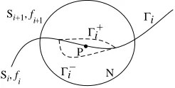
Let us now varyGiin a small neighbourhood of an arbitrary point P on contour Gi between two regions Si and SiC1 (as

shown in Fig. 1) and calculate variations of functional (1). Obviously, fi is varied in a neighbourhood N of P and these variations in fi are considered in the calculations of the functional variations.

Si+1, f_i+1

Si, f_i N

P Γi–

Γi+

Γi

IfGiis varied toGCi andG

K

i in the neighbourhood N of point

P shown inFig. 1, the variations of functional (1) are calculated as

EC_ðfC;

GC_Þ Z 1 2 X i ðð RC iKGC_i

½ðfC

i ðx;yÞKIðx;yÞÞ

2

CmðVf C

i Þ2S

C

i ðx;yÞdxdy

EK_ðfK;_GK_Þ

Z1 2 X i ðð RK iKGK_i

½ðfK

i ðx;yÞKIðx;yÞÞ

2

CmðVfKi Þ

2_SK

iðx;yÞdxdy

dEZECKEKZ1

2

XiC1

jZi

ðð

RC jKGC_j

½ðfC

j ðx;yÞKIðx;yÞÞ

2

CmðVfjCÞ

2

SC

j ðx;yÞdxdyK

1 2

!

XiC1

jZi

ðð

RK jKGK_j

½ðfK

j ðx;yÞKIðx;yÞÞ

2

CmðVf K

j Þ2S

K

jðx;yÞdxdy

or

dEZ1

2

ðð

RC igRCiC1KGC_i

½ðfC

ðx;yÞKIðx;yÞÞ2

CmðVf C

Þ2_SC

ðx;yÞdxdyK1

2

!

ðð

RK igR

K iC1KGK_i

½ðfK_ðx;_yÞKIðx;_yÞÞ2

CmðVfKÞ2SKðx;yÞdxdy

dEZ

1 2

ðð

N

½ðfC_ðx;_yÞKIðx;_yÞÞ2

CmðVfCÞ2

KðfK

ðx;yÞKIðx;yÞÞ2KmðVfKÞ2dxdy (6)

wherefC

andfK

are defined as:

fC Z

fC

i ðx;yÞ2N&ðx;yÞ2Ri

fC

iC1 ðx;yÞ2N&ðx;yÞ2RiC1

unchanged ðx;yÞ_;N

8 > > < > > : fK Z fK

i ðx;yÞ2N&ðx;yÞ2Ri

fK

iC1 ðx;yÞ2N&ðx;yÞ2RiC1

unchanged ðx;yÞ;N

8 > < > :

If we represent contourGias a natural representationGiZ

Gi(x(s),y(s)), then GCi can be represented as either

GC

i ZG

C

iðxðsÞ;yðsÞCmdyðsÞ=2Þ or G

C

i ZG

C

i ðxðsÞCmdxðsÞ=2;

yðsÞÞ.GK

i can be represented by the same form asG

C

i. Using

the first form forGC

i andG

K

i, Eq. (6) can, therefore, be rewritten

as

dEZ1

2

ðyCmðdy=2

yKmdy=2

½ðfC_ðx;_yÞKIðx;_yÞÞ2

CmðVfCÞ2

KðfK_ðx;_yÞKIðx;_yÞÞ2

KmðVfKÞ2dydx

or

dE

dGi

ZLim

m/0

dE m Z 1 2 ð N ½ðfC

ðx;yÞKIðx;yÞÞ2CmðVfCÞ2

KðfK

ðx;yÞKIðx;yÞÞ2 KmðVf

K Þ2_dydx

In order to find the condition under which functional (1) is optimised with respect to the variations of Gi, the above equation is set to 0, i.e.

ð

N

½ðfC_ðx;_yÞKIðx;_yÞÞ2

CmðVfCÞ2KðfKðx;yÞKIðx;yÞÞ2

KmðVfKÞ2dydxZ0

Sincedyis not zero in the neighbourhood N, we obtain

ðfC

ðx;yÞKIðx;yÞÞ2CmðVfCÞ2KðfKðx;yÞKIðx;yÞÞ2

KmðVfKÞ2Z0

(7)

The geometrical concept of Eq. (7) is that the contourGiis the intersection between two surfaces ðfCðx;yÞKIðx;yÞÞ2

C

mðVfC_Þ2

andðfK_ðx;_yÞKIðx;_yÞÞ2

CmðVfKÞ2. Although the two

surfaces have common points in continuous regions, however, in the neighbourhood of discontinuity, they only intersect at the contourGi. Eqs. (4), (5) and (7) can also be extended to obtain optimised solutions for the case where Gi is any nonclosed curve, i.e. they optimise functional (2) as well.

3. Implementation method

Original image can be approximated by minimising linear functional (8) to obtain a smooth and differentiable surface

f(x,y):

EðfÞZ1

2

X ðð

R

½ðfðx;yÞKIðx;yÞÞ2CmðVfÞ2dxdy (8)

By optimising functional (8) using Euler–Lagrange equation, the following differential equation is obtained:

mV2f ZfKI (9)

The solution for the above partial differential equation can be considered as a smooth differentiable Monge patch represented as[11,12]:

Sðx1_;

x2Þ_Zx1e1Cx2e2Cfðx 1_;

where (x1,x2) are coordinates corresponding to (x,y) ande1,e2, e3are unit vectorsi,jandkin a Euclidean manifold of three dimensions. This surface can be described using Gauss differential equations in tensor notation as (chapter 10 in [11]pp. 201–215, chapter 4 in[12] pp. 231–237)

vivjSZG k

ijvkSCbijN ði;j;kZ1;2Þ (11)

whereGkij are Christoffel symbols of the second kind, bij are components of a covariant tensor field of rank two representing the second fundamental coefficients of surfaces and Nis the unit normal vector to the surface. In Eq. (11), Einstein summation convention is employed (chapter 1 in [26]). Christoffel symbols are computed by the first fundamental coefficients or metric tensors represented by gij and their derivatives [11,12]. Therefore, according to Eq. (11), a surface can be uniquely determined by using its metric tensors and tensors representing its second funda-mental coefficients (chapter 10 in[11] pp. 203–208). In this paper, an algorithm is proposed to detect edges represented as discontinuities of the original imageI(x,y), by considering the smooth surface calculated from Eq. (9).

Normal curvature in any point on a smooth surface with metric tensors gij and the second fundamental coefficients tensorsbijis calculated as (chapter 9 in[11]pp. 179–181)

knZ

b11ðdx1Þ2C2b12dx1dx2Cb22ðdx2Þ2 g11ðdx1Þ2C2g12dx1dx2Cg22ðdx2Þ2

(12)

where dx1:dx2is the orientation along which normal curvature is computed. On the smooth surface obtained by solving Eq. (9), normal curvature along an orientation perpendicular to the tangent of the contour representing discontinuity is zero. This can further be investigated in Eq. (12), by substitutingXZdx1/dx2

knZ

b11X2C2b12XCb22 g11X2C2g12XCg22

Zero value for normal curvature requires that

b11X2C2b12XCb22Z0 (13)

In general, if bijs0, there is only one orientation along which normal curvature is zero. This is the orientation normal to the contour. Therefore, Eq. (13) should have only one single real root with multiplicity two. This is achieved when the discriminant of Eq. (13) is zero, i.e.:

b212Kb11b22Z0 (14)

Quantity b212Kb11b22 is a GI property of surfaces and is known as covariant Riemann tensor curvature. Orientation, along which normal curvature is zero, is the single real root of Eq. (13). This orientation is normal to edge path and calculated as:

XZK

b12 b11

(15)

Eq. (15) could be used to apply boundary condition of Eq. (5) on edge paths and contours. The condition indicated in

Eq. (14) can also be obtained by considering zero value for one of the principle curvatures. This implies that the Gaussian curvature of the surface in the point in question should be zero and hence condition (14) is satisfied. Such points on the surface are known as parabolic points (chapter 9 in[11]pp. 175–187). The other principle curvature then determines the curvature of the contour.

Area element on a smooth surface is another GI property that is used to detect discontinuities in the original image. On a smooth surface of an image, discontinuities correspond to regions with maximum area element on the smooth surface. For a surface with metric tensorgij, area element on the surface is calculated as the discriminant of metric tensor

gZ

jDSj Dx1_Dx2Z

ffiffiffiffiffiffiffiffiffiffiffiffiffiffiffiffiffiffiffiffiffiffiffiffi

g11g22Kg212

q

(16)

Therefore, if we start from a smooth surface obtained from Eq. (9), the edges correspond to points where Riemann tensor curvature is zero and Eq. (16) is maximised. Riemann curvature tensor and area variation calculated by Eq. (16) are initially computed for the whole image. Maximum values for this quantity in regions of zero Riemann curvature correspond to edges in the image. Since discriminant of metric tensor is definite positive, its minimum value is one corresponding to points with no variations. Therefore, a point is considered edge point if its tensor curvature is zero, its area is a local maximum and this maximum value is greater than a threshold.

Having segmented the image, Eq. (4) with the boundary condition (5) is applied to reduce the noise from the original image. To implement this noise reduction process, we start from the segmented image. For every pixel located ati,ja 3!3

window whose centre is at i, j is considered. If there is no segmented pixel in this window, the value of pixel ati,jfor the smoothed image is calculated using the discrete version of Eq. (4) estimated by finite difference method[14], i.e.

fði;jÞZmðfðiK1;jÞCfðiC1;jÞCfði;jK1ÞCfði;jC1ÞÞ

4mC1

C Iði;jÞ

4mC1

where I(i,j) is the pixel value at i, j from the noisy image. However, if any of the pixels’ locations at (iK1,j), (i,jK1), (iC1,j), and (i,jC1) are segmented, then the second derivative in Eq. (4) is estimated using the pixel values of the unsegmented pixels. For instance if the pixel at location (iK

1,j) is segmented, the pixel value of the smoothed image at location (i,j) is estimated as:

fði_;jÞ_ZmðfðiC1;jÞCfði;jK1ÞCfði;jC1ÞÞ

3mC1

C Iði_;jÞ

3mC1

depending on how close their pixel value is to f(i,j). This method guarantees sharp edges in a neighbourhood of an edge path in the smoothed image. Calculation methods of parameters bij, gij and curvature tensor are presented in the Appendix.

4. Results

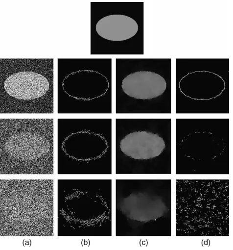
A noiseless synthetic image shown in Fig. 2(a), is contaminated with Gaussian noise to obtain a noisy image shown in Fig. 2(b) with SNRZ4.2. The GI based algorithm

described in Section 3 is applied to this noisy image. The segmented images are depicted inFig. 2(c)-(e) and smoothed images obtained by applying Eq. (4) with boundary condition (5) is shown in Fig. 2(f)-(h). mZ0.1, 5, and 50 are used to

smooth the noisy image. As shown from this figure, segmentation is unaffected for values of m higher than a threshold depending on the SNR of the image.

Values of mlower than this threshold result in partial or under segmentation, as shown inFig. 2(c). This is due to the fact that with low values ofm, edges as well as some portions of noise in the image have the required geometrical properties for segmentation. However, by increasing m, the required geometrical properties for edges remain unchanged, while noise is heavily smoothed which results in changes in their geometrical properties. This also suggests that small objects of the order of few pixels such as noise might not be detected when a high value ofmis chosen. It is, therefore, concluded that higher values formshould be chosen when the amount of noise in an image is increased. A smoother image is also obtained when higher values ofmare chosen. This is demonstrated in Fig. 2(f)–(h).

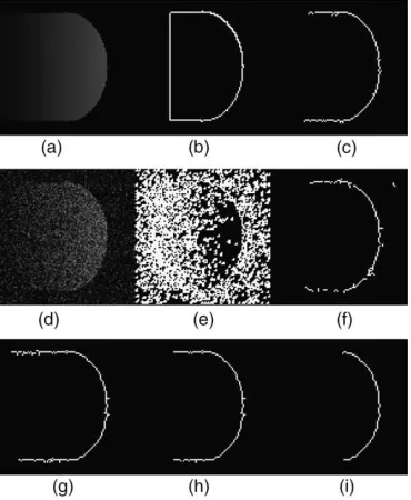
Contour of objects in images can also be open. Fig. 3(a) shows an image containing an object with a nonclosed contour. Gaussian noise is added to this image to obtain the image of Fig. 3(d) with SNRZ1. The edge detected images using an

iterative method implementing Mumford–Shah functional [6,17–20] and GI method are depicted in Fig. 3(b) and (c), respectively.

As shown in Fig. 3(b), the detected contour using this iterative algorithm is a closed contour, i.e. one part of the resulting contour does not actually exist as an edge in the original image. This is basically an artefact of the iterative method. This problem is resolved in the GI algorithm as seen in Fig. 3(c). The iterative method proposed in[6,17–20]and GI algorithm is applied to the noisy image ofFig. 3(d). While the GI algorithm successfully segments the image as depicted in Fig. 3(f), the iterative method which is operational for a favourable SNR, fails to segment the image as demonstrated in Fig. 3(e). The GI algorithm with different threshold values is applied to the noiseless image ofFig. 3(a), and the results are shown inFig. 3(g)–(i).

At this stage, it is interesting to investigate the noise sensitivity of our algorithm and compare this method to the derivative of Gaussian (DroG) edge detection algorithm[13]. An original noiseless image is contaminated with Gaussian noise with different variances to obtain noisy images with SNRZ0.5, 0.25, 0.03 as depicted inFig. 4. The proposed GI

algorithm in this paper is applied to the noisy images to obtain the segmented images. Noise reduction is also achieved by applying Eq. (4) with boundary condition (5) as shown in Fig. (4). Edge detection algorithm based on DroG is finally Fig. 2. Original noiseless image (a) noisy image contaminated with Gaussian

noise with SNRZ4.2 (b) Segmented image using the GI algorithm described in Section 3 usingmZ0.1 (c),mZ5 (d) andmZ50 (e) smoothed image withmZ 0.1 (f),mZ5 (g) andmZ50 (h).

applied to the noisy images for comparison. It should be noted that in both cases, empirically optimised threshold values were used for fair comparison. The window size for this DroG

algorithm is chosen as 9!9 and empirically optimal standard

deviations of the Gaussian function is chosen. As can be seen fromFig. (4),DroGoperator starts failing for the noisy image with SNRZ0.25. This failure is more clear for the noisy image

with SNRZ0.03. A better performance of GI algorithm than

that of theDroGoperator is clearly observed from this figure. This point is further investigated inFig. 5. It should be noted that noise reduction is considered as a by-product of our method. This bonus however is absent in the DroG edge detector.

A further comparison has been made between the DroG

edge detector and GI algorithm as depicted in Fig. 5. A noiseless image of Fig. 5(a) is contaminated with Gaussian noise to obtain a noisy image with SNRZ0.28 as shown in

Fig. 5(b). This image is segmented using the DroG edge

detector with two different threshold values. The other parameters are chosen empirically optimal. As can be seen fromFig. 5(b) and (c), if the threshold is chosen so that a closed contour is obtained for the object, noise is also segmented in some parts of the image as depicted inFig. 5(c). If the threshold increases to remove the ‘segmented noise’, then according to Fig. 5(d), the segmentation does not result in a close contour as expected. The GI algorithm is also applied to the noisy image of Fig. 5(b), and the segmented image includes a closed contour with virtually not segmented noise as depicted in Fig. 5(e). This clearly indicates a better performance for the GI algorithm compared to theDroGedge detector.

For comparison, the proposed GI algorithm in this paper and aDroGbased edge detector have been applied to a real world image, a noisy image of polymersomes cells. As depicted in Fig. 6, DroG edge detector using empirically optimised parameters partially segment the objects and fail to avoid detecting noise. However, better segmentation result is achieved by using the GI algorithm. The smoothed image is calculated withmZ100. GI algorithm has also been applied to

Lena, Cameraman, and Golden gate images contaminated with Gaussian noise with SNRZ10.25, 5.81 and 8.25, respectively.

Segmentation and smoothing are achieved bymZ5 as shown in

Figs. 7–9.

5. Conclusion

A nonlinear functional is introduced in this paper for segmentation and noise reduction of images. The proposed functional is less complex than the Mumford–Shah functional, and its implementation is consequently numerically more efficient. A noniterative method based on intrinsic properties of Fig. 4. Original noiseless image (top) noisy images contaminated with Gaussian

noise with SNRZ0.5, 0.25 and 0.03 (column a) segmented images using the proposed GI algorithm (column b) smoothed images using the proposed algorithm (column c) segmented images using DroG edge detector with window size 9!9, and empirically optimised standard deviations and threshold values (column d).

Fig. 5. Original noiseless image (a), noisy image with SNRZ0.28 (b) segmented image usingDroGoperator with different threshold values (c) and (d) segmented image using GI algorithm withmZ100 (e).

a differentiable surface approximating the original image is proposed. Results indicate that this method is very robust in the presence of noise and more effective than methods based on

DroG such as the Canny operator. The proposed method is generic and can be applied to signals and 3D images for segmentation and noise reduction.

Appendix

In this appendix, we calculate metric and curvature tensor by assuming that the differentiable surface is a Monge patchS. Normal unit vectorN,bijandgijare calculated as[11,12]:

g11Zv1S$v1SZðe1Cf;1e3Þ$ðe1Cf;1e3ÞZ1Cf;21

g12Zv1S$v2SZðe1Cf;1e3Þ$ðe2Cf;2e3ÞZf;1f;2

g22Zv2S$v2SZðe2Cf;2e3Þ$ðe2Cf;2e3ÞZ1Cf 2 ;2

NZ

v₁S!v2S jv1S!v2Sj

ZKf;1effiffiffiffiffiffiffiffiffiffiffiffiffiffiffiffiffiffiffiffiffiffiffiffi1Kf;2e2Ce3

1Cf_;2₁Cf_;2₂

q

b11Zv 2

1S$NZ ffiffiffiffiffiffiffiffiffiffiffiffiffiffiffiffiffiffiffiffiffiffiffiffif;11

1Cf2 ;1Cf;22

q

b12Zv1v2S$NZ ffiffiffiffiffiffiffiffiffiffiffiffiffiffiffiffiffiffiffiffiffiffiffiffif;12

1Cf_;2₁Cf_;2₂

q

b22Zv 2

2S$NZ ffiffiffiffiffiffiffiffiffiffiffiffiffiffiffiffiffiffiffiffiffiffiffiffif;22

1Cf2 ;1Cf_;2₂

q

wheref;iZvf/vx i

andf;ijZv 2

f/vxjvxi. Riemann curvature tensor and discriminant of metric tensor can therefore be rewritten as

RZb212Kb11b22Z

f;212Kf;11f;22 1Cf_;2₁Cf_;2₂

Fig. 7. Lena image (top left) and its noisy image contaminated with the Gaussian noise with SNRZ10.25 (top right) segmented and smoothed images using the GI method withmZ5 (bottom left and right, respectively).

Fig. 8. Cameraman image (top left) and its noisy image contaminated with the Gaussian noise with SNRZ5.81 (top right) segmented and smoothed images using the GI method withmZ5 (bottom left and right, respectively).

gZ

ffiffiffiffiffiffiffiffiffiffiffiffiffiffiffiffiffiffiffiffiffiffiffiffi

g11g22Kg212

q

Z

ffiffiffiffiffiffiffiffiffiffiffiffiffiffiffiffiffiffiffiffiffiffiffiffi

1Cf2 ;1Cf_;2₂

q

To find the points inx1x2plane where g is maximum, the zero-crossing in the directional derivative along unit vector normal to contour, i.e.vg/vn is examined. To ensure that in edge candidate points, g is maximised, v2g/vn2 should be negative. This can be written as:

vg

vnZ

ð

Vg$nZðg;1e1Cg;2e2Þ

$

g;1

ffiffiffiffiffiffiffiffiffiffiffiffiffiffiffiffiffi

g2_;1Cg2_;2

q e1C

g;2

ffiffiffiffiffiffiffiffiffiffiffiffiffiffiffiffiffi

g2_;1Cg2_;2

q e2

0 B @

1 C

AZ

ffiffiffiffiffiffiffiffiffiffiffiffiffiffiffiffiffi

g2 ;1Cg2;2

q

v2_g

vn2 Z

v vn

vg

vn Z

ð V vg

vn $n

Z g;1g;11ffiffiffiffiffiffiffiffiffiffiffiffiffiffiffiffiffiCg;2g;12 g2

;1Cg2_;2

q e1C

g;1g;12Cg;2g;22

ffiffiffiffiffiffiffiffiffiffiffiffiffiffiffiffiffi

g2 ;1Cg2_;2

q e2

0 B @

1 C A

$

g;1

ffiffiffiffiffiffiffiffiffiffiffiffiffiffiffiffiffi

g2 ;1Cg2_;2

q e1C

g;2

ffiffiffiffiffiffiffiffiffiffiffiffiffiffiffiffiffi

g2 ;1Cg2_;2

q e2

0 B @

1 C A

Therefore, in edge points the following inequality should apply

v2g

vn2Z

g2_;1g;11C2g;1g;2g;12Cg2;2g;22 g2

;1Cg2_;2

!0

References

[1] M. Kass, A. Witkin, D. Terzopoulos, Snakes: active contour models, Int. J. Comput. Vis. 1 (1987) 321–331.

[2] D. Mumford, J. Shah, Optimal approximations by piecewise smooth functions and associated variational problems, Commun. Pure Appl. Math. 42 (4) (1989) 577–688.

[3] J.M. Morel, S. Solimini, Variational Methods in Image Segmentation with Seven Image Processing Experiments, Birkhauser, Boston, 1995. [4] G. Aubert, P. Kornprobst, Mathematical Problems in Image Processing:

Partial Differential Equations and the Calculus of Variations, Springer, New York, 2002.

[5] A. Tsai, A. Yezzi, A.S. Willsky, Curve evolution implementation of the Mumford–Shah functional for image segmentation, denoising, interp-olation and magnification, IEEE Trans. Image Process. 10 (8) (2001) 1169–1186.

[6] T.F. Chan, L.A. Vese, Active contours without edges, IEEE Trans. Image Process. 10 (2) (2001) 266–277.

[7] M. Hintermuller, W. Ring, An inexact-CG-type active contour approach for the minimization of the Mumford–Shah functional, J. Math. Imaging Vis. 20 (2004) 19–42.

[8] J.A. Sethian, Levet Set Methods: Evolving Interfaces in Geometry, Fluid Mechanics, Computer Vision and Material Science, Cambridge Univer-sity Press, Cambridge, 1996.

[9] U.B. Manderscheid, Introduction to the Calculus of Variations, Chapman & Hall, London, 1991.

[10] I.M. Gelfand, S.V. Fomin, Calculus of Variations, Prentice-Hall, New Jersey, 1963.

[11] M.M. Lipschutz, Theory and Problems of Differential Geometry, Schaum’s Outline Series, McGraw-Hill, New York, 1969.

[12] M.P. Carmo, Differential Geometry of Curves and Surfaces, Prentice-Hall, New Jersy, 1976.

[13] J. Canny, A computational approach to edge detection, IEEE Trans. Pattern Anal. Mach. Intell. 8 (6) (1986) 679–698.

[14] E. Kreyszig, Advanced Engineering Mathematics, Wiley, London, 1999. [15] V. Caselle, R. Kimmel, G. Sapiro, Geodesic active contours, Procedings of the Fifth International Conference on Computer Vision, IEEE Computer Society Press, Silverspring, MD, 1995, pp. 694–699. [16] V. Caselles, R. Kimmel, G. Saprio, Geodesic active contours, Int.

J. Comput. Vis. 22 (1) (1997) 61–79.

[17] L.A. Vese, T.F. Chan, A multiphase level set framework for image segmentation using the Mumford and Shah model, Int. J. Comput. Vis. 50 (3) (2002) 271–293.

[18] T.F. Chan, B.Y. Sandberg, L.A. Vese, Active contours without edges for vector-valued images, J. Vis. Commun. Image Rep. 11 (2000) 130–141. [19] T.F. Chan, L.A. Vese, Level set algorithm for minimising the Mumford– Shah functional in image processing, Proceedings of the IEEE Workshop on Variational and Level Set Methods in Computer Vision, 2001, pp. 161–168.

[20] L.A. Vese, Multiphase object detection and image segmentation, in: S. Osher, N. Paragios (Eds.), Geometrical Level Set Methods in Imaging, Vision, and Graphics, Springer, New York, 2003, pp. 175–194. [21] A.N. Tikhonov, V.Y. Arsenin, Solutions of Ill-posed Problems, Winston

& Sons, Washington, DC, 1977.

[22] L. Rudin, S. Osher, E. Fatemi, Nonlinear total variation based noise removal algorithms, Physica D 60 (1992) 259–268.

[23] W. Hinterberger, M. Hintermuller, K. Kunisch, M. von Oehsen, O. Scherzer, Tube methods for BV regularization, J. Math. Imaging Vis. 19 (2003) 219–235.

[24] S. Mahmoodi, B.S. Sharif, Noise reduction, smoothing, and time interval segmentation of noisy signals using an energy optimisation method, IEE Proceedings Vision, Image and Signal Processing, in press.

[25] S. Mahmoodi, B.S. Sharif, Signal segmentation and denoising algorithm based on energy optimisation, Signal Process. 85 (2005) 1845–1851. [26] D.C. Kay, Tensor Calculus, Schaum’s Outline Series, McGraw-Hill, New