A Utility-Based Sensing and Communication Model for a
Glacial Sensor Network
Paritosh Padhy, Rajdeep K. Dash, Kirk Martinez and Nicholas R. Jennings
School of Electronics and Computer Science,University of Southampton, Southampton, SO17 1BJ ,UK.{
pp04r,rkd02r,km,nrj
}@ecs.soton.ac.uk
ABSTRACT
This paper reports on the development of a utility-based mechanism for managing sensing and communication in co-operative multi-sensor networks. The specific application considered is that of GLACSWEB, a deployed system that uses battery-powered sensors to collect environmental data related to glaciers which it transmits back to a base station so that it can be made available world-wide to researchers. In this context, we first develop a sensing protocol in which each sensor locally adjusts its sensing rate based on the value of the data it believes it will observe. Then, we detail a communication protocol that finds optimal routes for relay-ing this data back to the base station based on the cost of communicating it (derived from the opportunity cost of using the battery power for relaying data). Finally, we em-pirically evaluate our protocol by examining the impact on efficiency of the network topology, the size of the network, and the degree of dynamism of the environment. In so doing, we demonstrate that the efficiency gains of our new proto-col, over the currently implemented method over a 6 month period, are 470%, 250% and 300% respectively.
Categories and Subject Descriptors
I.2.11 [Artificial Intelligence]: Distributed Artificial In-telligence, Multiagent systems, Coherence and coordination.
General Terms
Algorithms, Design, Experimentation
Keywords
Agents and ambient intelligence, agents and novel comput-ing paradigms, Agent-based sensor networks.
1.
INTRODUCTION
Multi-sensor networks are being deployed in a wide variety of application areas and, in particular, they have recently
Permission to make digital or hard copies of all or part of this work for personal or classroom use is granted without fee provided that copies are not made or distributed for profit or commercial advantage and that copies bear this notice and the full citation on the first page. To copy otherwise, to republish, to post on servers or to redistribute to lists, requires prior specific permission and/or a fee.
AAMAS’06 May 8–12 2006, Hakodate, Hokkaido, Japan.
Copyright 2006 ACM 1-59593-303-4/06/0005 ...$5.00.
been advocated for a number of environmental monitoring applications [8]. Moreover, there is an increasing interest in controlling these networks using multi-agent system tech-niques [7]. In this vein, we consider a particular sensor network, GLACSWEB [8], that we have deployed in the Brikdalsbreen glacier in Norway, and examine how it can be modelled as a (cooperative) multi-agent system. In this case, the two main tasks performed by the sensors (agents) are gathering data from the environment and communicat-ing it towards a central sink node (i.e. an agent that harvests data from all other agents). In general, the agents work to-wards the predefined system goal of maximising data collec-tion (hence the cooperative nature of the system). However, they are invariably constrained in at least one of the follow-ing dimensions: their available power, their communication bandwidth, their memory storage and their processing ca-pability. Of these, power is the most important since it is required for everything else. Thus, it directly influences the life-span of the agents and, hence, that of the system as a whole. Given this, we focus on developing a communica-tion and a sensing protocol for this network. Nevertheless, the solution we develop is also more broadly applicable to networks that have any form of limited power supply.
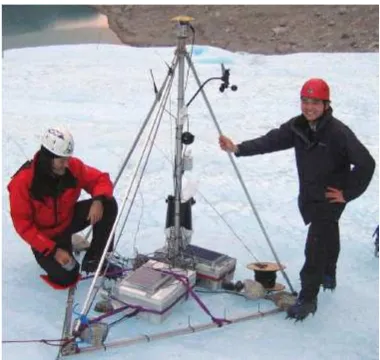
In more detail, the purpose of the GLACSWEB multi-sensor network is to monitor sub-glacial behaviour in or-der to unor-derstand climatic change. Figure 1 shows GLAC-SWEB’s central base station that is located on top of the glacier and figure 2 shows a typical GLACSWEB node. The individual nodes each sense their own data and then com-municate it directly to this sink node. As such, the sys-tem’s communication protocol is energy inefficient since it lacks the energy savings that a multi-hop approach would provide [12] (i.e. one in which agents relay data for one an-other). Furthermore, at present, sensing in GLACSWEB is carried out at a pre-determined constant rate which is blind to the actual variations in the environment. This decoupling results in unnecessary sampling because, given the same en-ergy expenditure, the information gained by sensing a slowly varying environment is less than what could be gained in a more dynamic situation.
Against this background, this paper develops a Utility-based Sensing and Communication protocol (called USAC). This consists of a sensing and a routing protocol that uses the cost of transmission and the value of observed data as utility metrics in the agents’ decision-making process. In doing so, we advance the state of the art in the following ways :
Figure 1: GLACSWEB base station Figure 2: A GLACSWEB sensor probe
In this, each agent adjusts its rate depending on the rate of change of its observations and a valuation func-tion (based on a sound informafunc-tion theoretic founda-tion) that the agents use for assigning a value to the data they observe.
• We devise a new routing protocol that finds the cheap-est cost route from an agent to the centre. Here, the cost of a link from one agent to another is derived us-ing the opportunity cost of the energy spent relayus-ing the data (i.e. the value that a relay could have gained by using the energy in sensing instead of relaying).
• We empirically evaluate the USAC protocol against the current GLACSWEB protocol and show that it introduces a significantly higher gain in information, whilst reducing power consumption.
The remainder of this paper is organised as follows. Sec-tion 2 provides some basic background on GLACSWEB and a discussion about related work in the area of sensor net-works modelled as multi-agent systems. We then detail the sensing protocol and the routing protocol of USAC in sec-tions 3 and 4 respectively. The USAC protocol is then em-pirically evaluated in section 5 in a wide range of scenarios. We conclude in section 6.
2.
BACKGROUND AND RELATED WORK
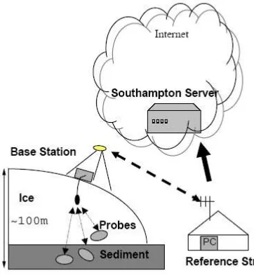
GLACSWEB is a deployed pervasive sensor network that directly monitors sub-glacial movement to determine how it is affected by climatic changes. In order to do this, it uses a network of sub-glacial probes which are placed at different locations inside the glacier as shown in figure 3.
The protocol currently followed by GLACSWEB is a sim-ple one in which the probes samsim-ple the glacier every four hours and then transmit these readings directly to the base station located at the top of the glacier daily. At this time, there are twenty probes in the glacier with an additional batch of ten deployed every summer. However, as a result of the hostile environment (due to the low temperatures, the strain resulting from moving ice and the englacial wa-ter bodies) and the power hungry protocol, there is a high
probe failure rate of around 50% per year. This provides the motivation for the research carried out in this paper.
Speaking more generally, it is widely recognised that there is a strong need for a well defined protocol stack in a sensor network that helps combine power and routing awareness, and that integrates data with the networking protocols. To this end, a number of routing protocols have been inves-tigated in this area. In particular, flooding [4] is one of the oldest and most common routing techniques. In flood-ing, each agent receives an item of data and then repeats it by broadcasting unless the destination of the packet is the agent itself. This is a reactive technique and does not require costly topology maintenance or complex route dis-covery algorithms. However, it can easily cause data im-plosion and/or data overlap which results in unnecessary wastage in communication power. The SPIN [5] routing protocol adopts a publish-subscribe approach to the prob-lem in which the agent nodes operate efficiently and conserve energy by all sending meta-data describing the sensor data instead of sending the actual data. Thus, this model is use-ful for those agents interested in the data advertised and is an effective protocol to minimise energy spent in consump-tion until the actual data is transmitted. However, it fails to place a limit on the energy consumed in wasted adver-tisements (i.e. for which there are no subscribers for the data). Moreover, the downside of both these models is that they involve significant amounts of communication and so consume large amounts of power which is often limiting.
To combat this, a number of researchers have focused on intelligent adaptive sensing [3]. Such work demonstrates that an active sensing approach can maximize a mobile sen-sor network’s lifetime by sensing only during the most infor-mative situations. However, our research differs from such approaches in that we focus on the sudden changes in the observed data rather than simply investigating regular pat-terns. In addition, our work reuses the utility derived from the sensing protocol in the communication protocol, thereby intertwining these two critical aspects of a sensor network. As a result, our model is sensor-centric, in contrast to the query-centric model adopted in [3].
[image:2.595.338.542.52.233.2]Figure 3: Architecture of the GLACSWEB network.
agents [2, 11]. In the latter case, the concept of selfishness arises mainly in those applications where agents are individ-ually owned by different stakeholders (which is not true in our case). The focus of our work is on cooperative agents (since all nodes are owned by one stakeholder, the Univer-sity of Southampton) and differs from existing research by combining the sensing and communication protocol via the utility function.
3.
THE SENSING PROTOCOL
In this section, we detail the sensing protocol of USAC which provides the agents with a sensing schedule. We concentrate here only on the sensing actions of an agent (thereby ignor-ing the communication actions dealt with in section 4 so as to simplify the exposition). This focus results in a single agent model in which the agent has to make optimal local decisions concerned with the timing of its sensing.
In more detail, the model for the sensing protocol is as follows. From the remaining battery energy, Ei, and the
energy,Esense, each sensing action takes1, agentican
cal-culate the maximum number of sensing actions,Nr s, it has
remaining (Nr
s = Ei/Esense). Given this, the agent then
needs to derive an optimal schedule for determining when
to carry out these actions. In order to do this, a metric is required to determine how well a particular schedule does compared to another. The metric we use in this case is derived frominformation-theory because this enables us to have a principled means of obtaining maximum information from the environment.
3.1
The Valuation Function
An optimal sampling rate can only be derived if the agent has knowledge about the future data. However, this require-ment is contradictory since in the case that the agent knows the future data, it does not need to sense the environment. As a result, an agent can only find an optimal sampling rate
1The sensors within GLACSWEB have the sameE
senseand
take the same amount of time to carry out one observation.
based on its forecast of the future data. Then, upon observ-ing previously forecasted data, the agent gains information by reducing its uncertainty about this data to zero. Here the representation we use for the uncertainty of the data is the confidence interval of a predicted data point. Specifically, thex% confidence interval of a data point is a range of val-ues centred around the mean of the forecast within which
x% of the data is guaranteed to fall. For example, a 100% confidence interval is the range of values the data can only ever take, whereas a 10% confidence interval implies that only 10% of the forecasted data is guaranteed to fall in this interval. From this, it can be seen that a lower confidence interval is more useful since its range is smaller. Therefore, a good forecast is one that minimises the confidence interval. The forecasting method we use here is based on a limited-window linear regression model. This is because it provides a good forecasting model for data that can be characterised as piecewise-linear functions of time with added Gaussian noise (which is the case for data collected in the GLACSWEB environment). Thus, the data can be represented by a set of equations of the form:
xTi+τ =αi+βiτ+η (1)
where{T1, T2, . . . , TI}represent the times at which a phase
change (i.e. a sudden variation in the data model) occurs,
αi+βiτ is the equation of the line after the phase change
at timeTi, andηis noise.
Thus, there are three major aspects of the data which are unknown:
• The current line segment equation (i.e. αi+βiτ).
• The time at which a phase change occurs (i.e.
{T1, T2, . . . , TI}).
• The level of noise in the environment (i.e. η).
Now, given observations (xb1, . . . ,bxn) taken at time (t1, . . . , tn),
a linear regression model of window sizemwould then esti-mateβias:
βi=
mP
m
i=lb(ti.xbi)− P
m i=lbti
P
m i=lbxbi)
nP
m i=lbt2i −
P
m i=lbti
2 (2)
where lb = max(n−m+ 1,1). Furthermore, using this model, we can estimateαias:
αi=
P
m
i=lbxbi−β
i
P
m i=lbti
n (3)
From this, the value at time intervalǫtafter the last mea-surement is predicted as:
xtn+ǫt=αi+βi(tn+ǫt) (4)
along with confidence intervals given by:
ci(tn) = 2σN(c/2) (5)
whereσis the standard deviation of the m samples andN(c) is the inverse of the positive part of the normal distribution function andc is the confidence level. Given this, we then calculate the value of a data point as:
Algorithm 1.
1. Observe data,nsample+ +
2. Ifnsample= 1thenV(data(ts)) =Vmax
3. If nsample = 2 then V(data(ts)) = Vmax, calculate
ci(ts)
4. Ifnsample>2then calculateci(ts) andV(data(ts))
• if data(ts) ∈ ci(ts−1) then fsample(ts) =
max(αfsample(ts−1), fmin)
• elsefsample(ts) =fmax andnsample= 1
[image:4.595.57.304.54.220.2]5. Go to Step 2
Figure 4: The sensing protocol algorithm.
whereci(ts−1) is the confidence interval before the data was sampled at timets andci(ts) is the confidence interval at
timetscalculated usingdata(ts). Having defined the sensing
protocol, we now turn to the algorithm to implement it.
3.2
The Algorithm
The algorithm we embed inside each agent for the sensing protocol is given in figure 4. The core concept behind this protocol is reflected in step 4. Here the reasoning is that if at timets the observed data falls outside the confidence
inter-val, then the agent should set its sampling ratefsampleto a
maximumfmax. This is because if the data falls outside the
interval then the agent believes that there has been a phase change in the environment. Hence it starts sampling at the most frequent rate in order to better incorporate this phase change in its forecasting model. However, if data falls within the confidence interval, it implies that the agent already has a good regression model. Hence, it can afford to reduce its sampling rate (represented in step 3 by the multiplicative factorα∈[0,1)) until the lower boundfminwhich has been
set by the requirements of the glaciologists. Steps 2 and 3 enable the agent to obtain the two data points required to carry out a linear regression.
4.
THE ROUTING PROTOCOL
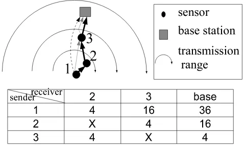
Once a sensor has collected data from the environment, it needs to transmit it towards the base station. So far, in GLACSWEB this is done by direct transmission to the cen-tre [10]. However, as discussed in section 2, this is inef-ficient since the power required to transmit data from one node to another is proportional to the square of the distance between the nodes (from basic radio transmission theory). As a result, the total energy spent by transmitting data directly to the centre via a single hop is more than the en-ergy spent when the data is relayed via successive interme-diaries to the centre. In order to see this effect, consider the example shown in figure 5. Here, sensor 1 could transmit data to the base station (bs) via the following three routes: 1→ 2→ 3 →bs (bold), 1 →3 → bs (grey) and 1→ bs
(broken line). The total energy consumed for the transmis-sion of one packet of data would then be 12 (4 + 4 + 4), 20 (16 + 4) and 36 respectively, thereby suggesting the use of route 1→2→3→bs.
Figure 5: Three possible routes via which sensor
1 can transmit its data to the base station. The concentric semi-circles show the range of sensor 1
with three power levels chosen such that the range grows linearly. The table shows the energy required for a sensor to transmit a packet directly to another.
However, an approach based solely on the transmission power is too na¨ıve since it disregards the two following as-pects:
1. The opportunity cost of the energy used by each sensor. If a sensor does not relay data, it could then use that energy in order to carry out additional sensing (which contributes towards the value of the network). Since each sensor is in a different local envi-ronment (due to the different placement of the sensors in the glacier), they derive different values by sens-ing the environment. Hence, it might be preferable for a sensor to transmit its data via a more energy-consuming route if the least energy-energy-consuming route contains a sensor in a highly dynamic environment.
2. The total power required to transmit along a particular route. The transmission of data also re-quires the receiving node to be in a listening mode (i.e. the agent needs to switch on its antenna for re-ceiving data which also consumes power). Thus the route 1→2→3→bsrequires both sensor 2 and 3 to additionally spend energy receiving the data.
We tackle these two problems by developing a utility-based communication protocol. This protocol is utility-based on the value of the data to be routed to the base station (which is derived according to section 3) and the cost of transmit-ting the data. We next detail how to calculate the cost of communication, before going onto the algorithm used for the communication protocol in section 4.2.
4.1
The Cost of Communication
The multisensor network is modelled as a multi-agent system consisting of a number of agents,I={1, . . . , n}, that each haveKdifferent discrete power levels,{pt1i, . . . , ptKi }, (with
ptk+1 i > pt
k
i) at which they can transmit. At each level,
there is a set of neighbours ni(ptki) ⊆ I to which agent i
can transmit data. Due to the nature of radio transmission,
ni(ptki)⊆ni(ptki+1).
Thus, the direct communication of data from any agent
[image:4.595.316.556.55.197.2]amount of energyEtji which is given by:
Etji(data) =pt k∗
i ×t j i(data)
where ptk∗
i is the lowest power level at which j ∈ ni(ptki)
andtj
i(data) is the amount of time a data packet takes to
transmit. Now, in this scenario the size of each sensed data packet and the bandwidth available to each agent is the same, sotj
i(data) is constant for all agents and sensed data
packets. Therefore, by slight abuse of notation, we shall hereafter refer toEtji(data) asEt
j i.
The cost of communication of an agentito another agentj
is then the opportunity cost of that decision. Now, there are two particular scenarios to consider when communicating data. If, on one hand, an agent is originating the data, then its cost of communication is given by:
cj
i(originate) =
Etj i
Etj
i+Esensei
×vsense
i (tn) (7)
whereEsense
i is the energy spent by iin sensing new data
andvsense
i (tn) is the value of the new data. On the other
hand, if an agent is relaying data, then its cost of transmis-sion is given by:
cj
i(relay) =
Etj i+E
receive i
Etj
i+Eisense
×vsense
i (tn) (8)
where Ereceive
i is the energy spent by the agent receiving
the data which it then relays.
Now, since it is not possible to assign vsense
i (tn) before
actually carrying out the observation, we need to estimate it. Due to the nature of the data (where sudden changes are possible) we estimatevsense
i (tn) using a moving average
with window sizew. Thus at timetnthe estimated value of
the data is given by:
visense(tn) =
1 min(n, w)
n−1
X
i=max(n−w,0)
vsensei (ti)
We choose such a forecasting method since it evens out the changes in value that random noise can introduce, whilst at the same time updating the value of the data fairly quickly as time progresses. However, it should be noted that this fore-casting method (or for that matter any forefore-casting method) cannot guarantee to correctly predict the value of the data all the time. Also, the moving average only starts once the number of samples collected by the sensor> w. Up to that point, the estimated value is just an average.
Having thus explained how the cost of communication is calculated, we now detail the algorithm followed by each agent when communicating data.
4.2
The Algorithm
The algorithm we use for the communication protocol is given in figure 6. It consists of four main steps, namely:
1. Initialisation. In this phase, the network topology is discovered and each agent is made aware of the power level it must transmit at in order to reach each of its neighbours. This phase is run each time probes are deployed within the glacier.
Algorithm 2.
1. Initialisation.
Run a network discovery protocol that establishes
ni(ptki) ∀k, i. Go to step 3.
2. Update transmission power.
At predefined intervals of time, tupdate (> 1/fmin),
the centre broadcasts a messagemsg0=hP0trans, P0reci
at the highest power level ptK
0, where P0trans is the
power at which the centre has transmitted this message and Prec
0 is the minimum power at which the centre
can receive data. An agent can then calculate the minimum power required to transmit to the centre as:
Pimin=
Prec
0 Pirec(msg0)
Ptrans 0
assuming that the dissipation of power is symmetric between 0 and i. From Pmin
i , an agent can then
determine the minimum power level ptk∗
i (0) required
to transmit to the base station (since 0 ∈ ni(ptki) if
ptk
i > Pimin ). It can then determine Et0i(data) and
thuscji(originate).
3. Update cost of transmission to base.
Let I(k∗) ∈ I be the set of agents that require the minimum power level ptk∗
i to transmit to base
(I(k∗) =n0(ptk0∗)−n0(ptk0∗−1))). Note thatpt00 ={0}.
Agentsi∈I(1)can calculate their own cost of relaying data to the base station, c0
i(relay). Upon calculation,
they broadcast the messagehc0
i(relay)i at power level
ptK i .
Then fork∗= 2toK do
• Agents i ∈ I(k∗) calculate the cost of relaying datacji(relay)to all agentsj∈I(k∗ −1).
• They also update their cost of transmission,
c0
i(originate), as min(cli(originate) +c0l(relay))
wherel∈ ∪k∗−1
a=1 I(k∗ −a)
• They then broadcast the message hc0 i(relay)i
at power level ptK
i where c0i(relay) =
min(cl
i(relay) +c0l(relay)).
4. Transmit data.
Send the data packet through the lowest cost path if Vi(data(ts)) > c0i(originate). Update
cji(originate), c j
i(relay) from the value of newly
sensed data. 5. Repeat Step.
Iftime to update transmission power levels,
thengo to Step 2
else iftime to update relay and originate costs
thengo to Step 3
elsesense data and go to step 4.
2. Update energy band of agent. This step is respon-sible for dividing the agents into different power level groups with respect to the base. This segmentation is then used in the next step in order to update the cost of relaying data.
3. Update cost of transmission to base. This step is required so as to find the minimum cost route from each agent to the centre. In order to do so, agents in each power level group successively transmit the cost of their cheapest route to the centre.
4. Transmit data. Having found the cheapest cost of transmission to the base, the agent then decides whether or not to transmit its observed data.
5.
EMPIRICAL EVALUATION
The aim of these experiments is to determine the relative performance of USAC when compared to the currently de-ployed GLACSWEB protocol. Now, the performance of any protocol in this scenario is contingent on a number of fac-tors such as the network topology, the number of agents within the network and the type of environment in which it is employed. Thus, in order to generalise our results, we benchmark the performance of USAC against GLACSWEB, whilst independently varying each of the factors mentioned above. We also calculate theefficiency(i.e. the value of the data gained over the energy consumed) of USAC relative to GLACSWEB in each case.
5.1
Experimental Setup
The GLACSWEB simulator lets each of the nodes take one of the following actions in a single time period:sense,idle−
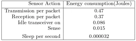
[image:6.595.52.291.603.676.2]listen(where an agent enables its antenna so that it is ready to receive data),transmita single packet,receivea single packet andsleep. With the exception oftransmit, all ac-tions have a set power consumption value affixed to them. The power consumption of thetransmitaction is dependent on the variable transmission power of the agent transmitter. Each such agent has five levels of transmission power to com-municate with agents at different transmission ranges. The radio propagation model in the simulation was assumed to be symmetric. We decided to ignore theprocessingaction of the agent due to its near negligible power consumption. Specifically table 1 shows the typical energy consumption of each action based on the values obtained from the fielded system. Furthermore, the energy capacity of the node was 77760 J and the confidence level within the sensing proto-col was set to 10% (again based on our experience with the fielded system).
Table 1: Energy consumption of sensor node actions
Sensor Action Energy consumption(Joules)
Transmission per packet 0.47
Reception per packet 0.37
Idle transceiver on 0.086
Sense 0.015
Sleep per second 0.000032
We also decided to use a simple version of the IEEE 802.11 Medium Access Control [9] where RTS/CTS2 control pack-2Request-To-Send/Clear-To-Send.
ets are only used before transmission of the data packets that are sent in a burst. Also there was no difference between overhearing and receiving in terms of power consumption. However, agents were programmed to ignore packets that were not destined to them and thereafter lower their power consumption by switching to the idle transceiver mode. In order to obtain statistically significant results, we report av-erage result and standard deviations of 200 simulations in each of the experiments carried out. The data used in our experiments are derived from segments of the data collected3 by the fielded probes over the last year.
5.2
Network Topology
In this experiment, we simulated the two protocols for a fixed number of agents (10) randomly distributed around the centre. The sensed data model for each agent and number of agents in the networks were fixed for each instance of the simulation. The purpose of this was to analyse how the two protocols fared against each other with the changing topology of the network. The results of these simulations are shown in the two plots in Figure 7.
Both plots show the superiority of USAC over GLAC-SWEB. The big jump at the beginning of USAC’s value graph is attributed to the maximum rate of sampling in the initial stages. Once a sufficient number of samples have been collected, the sampling rate is reduced and adjusted accord-ing to the change in observed data. The overall graphs of both protocols are linear. However, the gradient of USAC is steeper than that of GLACSWEB. This is because USAC increases its sampling whenever the observed data changes. The efficiency gain of USAC over GLACSWEB in this ex-periment was calculated to be 470%.
5.3
Network Size
In this experiment, we conducted simulations by varying the number of agents in the network from 1 to 20. Figure 8 illustrates the performance of USAC against GLACSWEB with varying network size. Due to the variability of the data, we concern ourselves with the average of the final total at the end of each simulation to ensure an effective comparison. As can be seen, USAC consistently consumes less energy and still manages to collect more valued data at the sink node (even as the size of the network is increased). How-ever, the random placement of the agent nodes results in a greater variance in the total value of data collected using USAC. This is due to the way that USAC reallocates the energy saved, when not relaying, to the task of sensing. In particular, the network topology in an instance of the exper-iment determines the amount of energy an agent spends on communication and therefore the amount of sensing it per-forms. In other words, an agent closer to the base station might relay and communicate more data since the value of the data derived might often be more than the cost of com-munication. On the other hand, an agent further away from the base station might be forced to communicate and relay less data because the cost of communication may now have surpassed the value of data it has sensed. The efficiency gain of USAC over GLACSWEB in this part of the experiment was calculated to be 250%.
0 50 100 150 200 0
2000 4000 6000 8000 10000 12000
Total energy consumed by all sensors over a 6−month period
time
Energy consumed
Glacsweb
USAC
(a) Energy Consumption
0 50 100 150 200
0 500 1000 1500 2000
Total value of data gathered over a 6−month period
time
Value of data
Glacsweb USAC Glacsweb data4
[image:7.595.122.481.70.218.2](b) Value Derived
Figure 7: The total energy spent and total data value gathered over a 6-month period plotted against time.
0 5 10 15 20
0 0.5 1 1.5 2 2.5
3x 10
4Total power spent at end of 6−month period
Number of agents
Power
Glacsweb USAC
(a) Energy Consumption
0 4 8 12 16 18
0 500 1000 1500 2000 2500 3000 3500 4000
Total value of data collected at base at end of 6−month period
Number of agents
Value of data
Glacsweb USAC
[image:7.595.126.480.282.434.2](b) Value Derived
Figure 8: The total energy spent and total data value gathered at the end of a 6-month period plotted against number of agents in the network
0 5 10 15 20 25
3000 4000 5000 6000 7000 8000 9000
Total energy spent at end of 6−month period
Number of phase changes in data
Energy
Glacsweb USAC
(a) Energy Consumption
0 5 10 15 20 25
0 2000 4000 6000 8000 10000
Total value of data collected at base at end of 6−month period
Number of phase changes in data
Value of data
Glacsweb USAC
(b) Value Derived
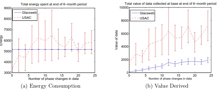
[image:7.595.123.486.510.661.2]5.4
Dynamism of the Environment
In this experiment, simulations were carried out by vary-ing the data model of the agent nodes whilst keepvary-ing the topology and size of the network constant. The degree of dynamism in the data model is defined as the number of phase changes that occur in the piecewise linear data model of the environment used by the agent. The results of these simulations are shown in figure 9.
The results from sub-figure 9(a) show that USAC adapts its power consumption based on the dynamism of the data (in contrast to GLACSWEB where the sensing protocol is static and unaffected by the type of data it is measuring). This results in the higher total value of data collected at the sink for USAC as shown in sub-figure 9(b). The high variance observed with USAC is due to the random times at which phase changes occur. Thus, if two phase changes oc-cur very close to each other, there is a possibility of misrep-resenting the changes which leads to low power consumption and low value. This experiment showed that USAC has an efficiency gain of 300% over GLACSWEB.
6.
CONCLUSIONS AND FUTURE WORK
The protocol we have developed in this paper allows agents to act in a decentralised (based on the nature of their local environment) manner, while self-organising to form a net-work whose performance is high in terms of minimising en-ergy consumption and maximising the value of data gained. It makes use of the localisation ability of individual agents to determine the cheapest cost path to the sink and incorpo-rates the value of the observed data to calculate the cheapest path. We have also shown that our protocol is superior to the currently deployed GLACSWEB protocol, even when the distribution of agents around the sink and the nature of observed environment is varied.
Whilst we have specifically considered evaluating the ef-fectiveness of our protocol in the GLACSWEB sensor net-work, the challenges involved here are very similar to those that occur in the design of many other sensor networks. For example, we are currently exploring the possibility of using it in the FloodNet system (a sensor network for monitoring river levels in which the sensors are solar powered)4. Also, in the current work, we have considered just one particular way of calculating the value of information. In future work, we wish to investigate whether more complicated information theoretic measures, such as Kullback-Liebler divergence and Mahanalobis distance, would be a better basis for measuring information and whether these more sophisticated measures would improve the system’s efficiency. It would also be inter-esting to introduce additional factors in the simulation such as network openness and scalability (where agents come and leave the system) and extend our protocol to accommodate this aspect of dynamism in the network.
7.
REFERENCES
[1] J. Byers and G. Nasser. Utility-based decision-making in wireless sensor networks. InProceedings of the first ACM international symposium on Mobile ad hoc networking & computing(MOBIHOC’00), pages 143–144, Piscataway, NJ, USA, 2000. IEEE Press. [2] R. Dash, A. Rogers, S. Reece, S. Roberts, and N. R.
Jennings. Constrained bandwidth allocation in 4http://envisense.org/floodnet/floodnet.htm
multi-sensor information fusion: a mechanism design approach. InProceedings of the 8th International Conference on Information Fusion, 2005.
[3] A. Deshpande, C. Guestrin, S. Madden, J. Hellerstein, and W. Hong. Model-based approximate querying in sensor networks.International Journal on Very Large Data Bases, 2005. To appear.
[4] P. Downey and R. Cardell-Oliver. Evaluating the impact of limited resource on the performance of flooding in wireless sensor networks. InProceedings of the International Conference on Dependable Systems and Networks (DSN’04), pages 785–794, 2004. [5] W. R. Heinzelman, J. Kulik, and H. Balakrishnan.
Adaptive protocols for information dissemination in wireless sensor networks. InProceedings of the ACM/IEEE International Conference on Mobile Computing and Networking (MobiCom’99), pages 174–185, 1999.
[6] B. Horling, R. Vincent, R. Mailler, J. Shen, R. Becker, K. Rawlins, and V. Lesser. Distributed sensor network for real time tracking. InProceedings of the Fifth International Conference on Autonomous Agents (AGENTS ’01), pages 417–424, New York, NY, USA, 2001. ACM Press.
[7] V. Lesser, C. Ortiz, and M. Tambe, editors.
Distributed sensor networks: a multiagent perspective. Kluwer Publishing, 2003.
[8] K. Martinez, J.K. Hart, and R. Ong. Environmental sensor networks.Computer, 37(8):50–56, 2004. [9] LAN MAN Standards Committee of the IEEE
Computer Society.Wireless LAN medium access control (MAC) and physical layer (PHY) specification. IEEE, New York, NY, USA, 802.11-1997 edition, 1997. [10] P. Padhy, K. Martinez, A. Riddoch, J.K. Hart, and
H.L.R. Ong. Glacial environment monitoring using sensor networks. InProceedings of the First Real-World Wireless Sensor Networks
Workshop(REALWSN’05), pages 10–14, 2005. [11] A. Rogers, E. David, and N. R. Jennings. Self
organised routing for wireless micro-sensor networks.
IEEE Transactions on Systems, Man and Cybernetics (Part A), 35(3):349–359, 2005.
[12] A. Woo, T. Tong, and D.Culler. Taming the underlying challenges or reliable multihop routing in sensor networks. InProceedings of the First
International Conference on Embedded Networked Sensor Systems (SenSys’03), pages 14–27, 2003.