The numerical simulation of ship waves using cartesian grid and volume of fluid methods

26th_{Symposium on Naval Hydrodynamics} Rome, ITALY, 17-22 September 2006

The numerical simulation of ship waves using cartesian-grid

and volume-of-fluid methods

Douglas G. Dommermuth

, Thomas T. O’Shea

, Donald C. Wyatt

,

Mark Sussman

, Gabriel D. Weymouth

, Dick K.P. Yue

,

Paul Adams

, and Randall Hand

Naval Hydrodynamics Division, Science Applications International Corporation, 10260 Campus Point Drive, MS 35, San Diego, CA 92121

2

Department of Mathematics, Florida State University, Tallahassee, FL 32306 3

Department of Mechanical Engineering, Massachusetts Institute of Technology, Cambridge, MA 02139 4

U.S. Army Engineer Research and Development Center, Vicksburg, MS 39180

Abstract

Numerical predictions are compared to experimental measurements of ship models moving with forward speed, including model 5415 and model 5365 (Athena). The ability to model forced-motions is illustrated using a heaving sphere moving with forward speed.

Introduction

The Numerical Flow Analysis (NFA) code provides turnkey capabilities to model breaking waves around a ship, including both plunging and spilling breaking waves, the formation of spray, and the entrainment of air. NFA uses a cartesian-grid formulation with immersed-body and volume-of-fluid (VOF) methods. The govern-ing equations are formulated on a cartesian grid thereby eliminating complications associated with body-fitted grids. The sole geometric input into NFA is a surface panelization of the ship hull. No additional gridding be-yond what is already used in potential-flow methods and hydrostatics calculations is required. The ease of input in combination with a flow solver that is implemented using parallel-computing methods permit the rapid turn around of numerical simulations of complex interactions between free surfaces and ships.

Based on Colella, Graves, Modiano, Puckett & Sussman (1999), free-slip boundary conditions are im-posed on the surface of the ship hull. The fractional areas and volumes of very small cells are merged to improve the conditioning of the Poission solver (Mampaey & Xu 1995). The grid is stretched along the cartesian axes using one-dimensional elliptic equations to improve res-olution near the ship hull and the free-surface interface. Away from the ship and the free-surface interface, where the flow is less complicated, the mesh is coarser. Details of the grid stretching algorithm, which uses weight func-tions that are specified in physical space, are provided in

Knupp & Steinerg (1993). Free-slip boundary conditions are also imposed at the entrance, along the sides, and at the top and bottom of the computational domain. At the exit, Orlanski-like boundary conditions are imposed (Orlanski 1976).

The VOF portion of the numerical algorithm is used to track the free-surface interface, including the large-scale effects of breaking waves, spray formation and air entrainment. A novel regridding scheme is introduced whereby the level of water at the entrance of the com-putational domain is preserved. The interface tracking of the free surface is second-order accurate in space and time. At each time step, the position of the free surface is reconstructed using piece-wise planar surfaces (Rider, Kothe, Mosso, Cerutti & Hochstein 1994, Gueyffier, Li, Nadim, Scardovelli & Zaleski 1999). The advection por-tion of the VOF algorithm uses an operator-split method (Puckett, Almgren, Bell, Marcus & Rider 1997). The advection algorithm implements a correction to improve mass conservation when the flow is not solenodal due to numerical errors.

The convective terms in the momentum equations are treated using a slope-limited, third-order QUICK scheme as discussed in Leonard (1997). A Smagorin-sky turbulence model is also implemented.. There are no special treatments required to model either the flow sepa-ration at the transom or the wave overturning at the bow. A second-order, variable-coefficient Poisson equation is used project the velocity onto a solenoidal field. A pre-conditioned conjugate-gradient method is used to solve the Poisson equation.

grid points and inversely proportional to the number of processors. For the most part, NFA performed equally well on the Cray X1, which is a vector machine, and the Cray XT3, which is a massively parallel machine. The main exception involved portions of NFA that involved conditional statements that could not be vectorized on the Cray X1. Together, the ease of input and usage, the ability to model and resolve complex free-surface phe-nomena, and the speed of the numerical algorithm pro-vide a robust capability for simulating the free-surface disturbances near a ship.

Formulation

Consider turbulent flow at the interface between air and water. Letuidenote the three-dimensional velocity field

as a function of space (xi) and time (t). The coordinate

system is fixed with respect to the ship.viis the velocity of the ship. viincludes the effects of rigid-body transla-tion and rigid-body rotatransla-tion. For an incompressible flow, the conservation of mass gives

∂ui

∂xi = 0 . (1)

uiandxiare normalized byUoandLo, which denote the free-stream velocity and the length of the body, respec-tively.

Following a procedure that is similar to Rider et al. (1994), we letφdenote the fraction of fluid that is inside a cell. By definition,φ= 0for a cell that is totally filled with air, and φ = 1for a cell that is totally filled with water.

The convection ofφis expressed as follows:

∂φ ∂t +

∂

∂xj[(ui−vi)φ] = ∂Q

∂xj , (2)

vi is the velocity of the body. The coordinate system is fixed with respect to the body (Repetto 2000). Qis a sub-grid-scale flux which can model the entrainment of gas into the liquid. Dommermuth, Innis, Luth, Novikov, Schlageter & Talcott (1998) provide details of a sub-grid model that is appropriate for interface capturing meth-ods that allow mixing of air and water. Since the present formulation maintains a sharp interface,Q= 0.

Let ρ` andµ` respectively denote the density and dynamic viscosity of water. Similarly,ρgandµgare the corresponding properties of air. The flows in the water and the air are governed by the Navier-Stokes equations:

dui

dt +

∂

∂xj[(ui−vi)uj] =−

1 ρ ∂P ∂xi + 1 ρRe ∂

∂xj (2µSij)− Gi F2

r

+∂τij

∂xj , (3)

whereRe = ρ`UoLo/µ` is the Reynolds number and

Fr2 =Uo2/(gLo)is the Froude number. gis the

acceler-ation of gravity. Gi is a body force that rotates with the body (Repetto 2000).Pis the pressure. As described in Dommermuth et al. (1998),τijis the subgrid-scale stress

tensor.Sijis the deformation tensor: Sij =

1 2 _∂ui ∂xj +∂uj ∂xi . (4)

ρandµare respectively the dimensionless variable den-sities and viscoden-sities:

ρ(φ) = λ+ (1−λ)H(φ)

µ(φ) = η+ (1−η)H(φ) , (5)

whereλ=ρg/ρ`andη=µg/µ`are the density and

vis-cosity ratios between air and water. For a sharp interface, with no mixing of air and water,His a step function. In practice, a mollified step function is used to provide a smooth transition between air and water.

A no-flux condition is imposed on the surface of the ship hull:

uini=vini (6)

whereni denotes the normal to the ship hull that points into the fluid.

As discussed in Dommermuth et al. (1998), the di-vergence of the momentum equations (3) in combina-tion with the conservacombina-tion of mass (1) provides a Poisson equation for the dynamic pressure:

∂ ∂xi

1

ρ ∂P

∂xi = Σ , (7)

where Σis a source term. As shown in the next sec-tion, the pressure is used to project the velocity onto a solenoidal field.

NUMERICALTIMEINTEGRATION

Based on Sussman (2003a), a second-order Runge-Kutta scheme is used to integrate with respect to time the field equations for the velocity field. Here, we illustrate how a volume of fluid formulation is used to advance the volume-fraction function Similar examples are pro-vided by Rider et al. (1994). During the first stage of the Runge-Kutta algorithm, a Poisson equation for the pres-sure is solved:

∂ ∂xi

1

ρ(φk₎ ∂P∗

∂xi =

∂ ∂xi

uk_i

∆t +Ri

, (8)

whereRidenotes the nonlinear convective, hydrostatic, viscous, sub-grid-scale, and body-force terms in the mo-mentum equations.uk

i andρkare respectively the

For the next step, this pressure is used to project the velocity onto a solenoidal field. The first prediction for the velocity field (u∗_i) is

u∗_i =uk_i + ∆t

Ri− 1

ρ(φk₎ ∂P∗

∂xi

(9)

The volume fraction is advanced using a volume of fluid operator (VOF):

φ∗=φk−VOF uk_i, φk,∆t

(10) Details of the VOF operator are provided later. A Pois-son equation for the pressure is solved again during the second stage of the Runge-Kutta algorithm:

∂ ∂xi

1

ρ(φ∗₎ ∂Pk+1

∂xi =

∂ ∂xi

u∗_i +uk_i

∆t +Ri

(11)

uiis advanced to the next step to complete one cycle of the Runge-Kutta algorithm:

uk_i+1= 1 2

u∗_i +uk_i + ∆t

Ri−

1

ρ(φ∗₎ ∂Pk+1

∂xi

,(12)

and the volume fraction is advanced to complete the al-gorithm:

φk+1=φk−VOF

_u∗ i +uki

2 , φ

k ,∆t

(13)

GRIDDING

Along the cartesian axes, one-dimensional stretch-ing is performed usstretch-ing a differential equation. Letx de-note the position of the grid points in physical space, and letξdenote the position of the grid points in a mapped space. As shown by Knupp & Steinerg (1993), the dif-ferential equation that describes grid stretching in one di-mension is as follows:

∂2_x

∂ξ2 + 1

w ∂w

∂ξ ∂x

∂ξ = 0 , (14)

wherew(x)is a weight function that is specified in phys-ical space. For example, suppose the grid spacing is con-stant but different for x < xo andx > x1. Between

xo ≤ x ≤ x1, there is a transition zone from one grid spacing to the next. Then the following weight function may be used to describe this distribution of grid points:

w(x) = w0 for x < x0

w(x) = w0−w1 2

1 + cos(π(x−x0)

x1−x0 )

+ w1 for x0≤x≤x1

w(x) = w1 for x > x1 . (15)

Using this approach, multiple zones of grid clustering may be specified. For example, along the x-axis (x1in indical notation), grid points may be clustered near the bow and stern. For the y-axis (x2 in indical notation), grid points are clustered near the centerline out beyond the half beam. Finally, for the z-axis (x3in indical no-tation), grid points are clustered near the mean waterline in a region that is between the top and bottom of the ship hull. Note that equation 14, is a nonlinear equation that is solved iteratively.

ENFORCEMENT OFBODYBOUNDARYCONDITIONS

A no-flux boundary condition is imposed on the sur-face of the body using a finite-volume technique. A signed distance functionψis used to represent the body.

ψ is positive outside the body and negative inside the body. The magnitude of ψis the minimal distance be-tween the position ofψand the surface of the body.ψis zero on the surface of the body. ψis calculated using a surface panelization of the hull form. Green’s theorem is used to indicate whether a point is inside or outside the body, and then the shortest distance from the point to the surface of the body is calculated. Triangular panels are used to discretize the surface of the body. The shortest distance to the surface of the body can occur on either a surface, edge, or vertice of a triangular panel. Details associated with the calculation ofψare provided in Suss-man & Dommermuth (2001).

Cells near the ship hull may have an irregular shape, depending on how the surface of the ship hull cuts the cell. On these irregular boundaries, the finite-volume ap-proach is used to impose free-slip boundary conditions. LetSbdenote the portion of the cell whose surface is on the body, and letSodenote the other bounding surfaces of the cell that are not on the body. Gauss’s theorem is applied to the volume integral of equation 8:

Z

So+Sb

ds ni

ρ(φk₎ ∂P∗

∂xi

=

Z

So+Sb

ds

_uk ini

∆t +Rini

.(16)

Here,ni denotes the components of the unit normal on

the surfaces that bound the cell. Based on equation 9, a Neumann condition is derived for the pressure onSb as follows:

ni ρ(φk₎

∂P∗

∂xi =−

u∗_ini

∆t + uk_ini

∆t +Rini . (17)

The Neumann condition for the velocity (6) is substituted into the preceding equation to complete the Neumann condition for the pressure onSb:

ni ρ(φk₎

∂P∗ ∂xi

=−v ∗ ini

∆t + uk

ini

This Neumann condition for the pressure is substituted into the integral formulation in equation 16:

Z

So

ds 1

ρ(φk₎ ∂P∗

∂xi ni =

Z

So

ds

uk_ini

∆t +Rini

+ Z Sb dsv ∗ ini

∆t (19)

This equation is solved using the method of fractional areas. Details associated with the calculation of the area fractions are provided in Sussman & Dommermuth (2001) along with additional references. Cells whose cut volume is less than 25% of the full volume of the cell are merged with neighbors. The merging occurs along the direction of the steepest gradient of the signed-distance functionψ. This improves the conditioning of the Pois-son equation for the pressure. As a result, the stability of the projection operator for the velocity is also improved (see equations 9 and 12).

INTERFACE RECONSTRUCTION AND ADVECTION

In our VOF formulation, the free surface is recon-structed from the volume fractions using piece-wise lin-ear polynomials. The reconstruction is based on algo-rithms that are described by Gueyffier et al. (1999). The surface normals are estimated using weighted central dif-ferencing of the volume fractions. A similar algorithm is described by Pilliod & Puckett (1997). Near the body, care must be taken to use cells whose volume fraction is exterior to the body in the calculation of the normal to the free-surface interface. The advection portion of the algorithm is operator split, and it is based on similar al-gorithms reported in Puckett et al. (1997). Major differ-ences between the present algorithm and earlier methods include special treatments to account for the body and to alleviate mass-conservation errors due to the presence of non-solenoidal velocity fields.

LetFidenote flux through the faces of a cell. Fi is

expressed in terms of the relative velocity (ui−vi) and

the areas of the faces of the cell (Ai) that are cut by the ship hull:

Fi=Ai(ui−vi) . (20)

If the ship hull does not cut the cell, thenAicorrespond to the surface areas that bound the cell. Near the ship hull,Aiis some fraction of the surface areas that bound the cell. Note thatAi= 0inside the ship hull. Based on an application of Gauss’s theorem to the volume integral of Equation 1 and making use of Equation 6:

F_i+−F_i−= 0 , (21)

whereF_i+is the flux on the positive i-th face of the cell andF_i− is the flux on the negative i-th face of the cell.

Due to numerical errors, equation 21 is not necessarily satisfied. LetE denote the resulting numerical error for any given cell. For each cell whose flux is not conserved, a correction is applied prior to performing the VOF ad-vection. For example, the following reassignment of the flux along the vertical direction ensures that the redefined flux is conserved:

˜

F₃+ = F₃+− EA + 3

A+₃ +A−₃

˜

F₃− = F₃−+ EA

−

3

A+₃ +A−₃ (22)

Based on this new flux, new relative velocities are de-fined on the faces of the cell:

ˆ

ui =

∆xiF˜i

V (23)

where∆xi is the grid spacing and V = ∆x1∆x2∆x3 is the volume of the cell. Away from the ship hull, uˆi

is the relative velocity with a corrective term to conserve mass. Inside the ship hull,uiˆ = 0becauseAi= 0. Near the ship hull,uiˆ is scaled by the fraction of area that is cut by the presence of the ship hull. uiˆ is continuous across the faces of the cells along x−andy−axes, but discontinuous across the faces along thez−axis because in this particular example that is the axis where the flux has been corrected.

Equation 2 is operator split. A dilation term is added to ensure that the volume fraction remains between0≤ φ ≤ 1during each stage of the splitting (Puckett et al. 1997). The resulting discrete set of equations for the first stage of the time-stepping procedure is provided below:

˜

φ=φk −

F1

h

ˆ

u+₁k, φk,∆ti− F1

h

ˆ

u−₁k, φk,∆ti

V

+ ∆tφ˜ uˆ

+ 1

k

− uˆ−₁k

∆x1

˜˜

φ= ˜φ − F2

h

ˆ

u+₂k,φ,˜ ∆ti− F2

h

ˆ

u−₂k,φ,˜ ∆ti

V

+ ∆tφ˜˜ uˆ

+ 2

k

− uˆ−₂k

∆x2

φ∗=˜˜φ − F3

h

ˆ

u+₃k,φ,ˆ ∆ti− F3

h

ˆ

u−₃k,φ,ˆ ∆ti

V

+ ∆tφ˜˜ uˆ

+ 3

k

− uˆ−₃k ∆x3

, (24)

Fi denotes VOF advection based on the uncut areas of

the preceding equation. Note that the order of the split-ting is alternated from time step to time step to preserve second-order accuracy.

The free-surface interface that is reconstructed from the volume fractions is most often calculated and visual-ized using commercial codes. Specifically, commercial codes calculate the 0.5 isosurface of the volume-fraction functionφ. The free-surface interface that is calculated from the 0.5 isosurface is different from the free-surface interface that is reconstructed from the volume fractions. To illustrate this point, consider a cell whose volume fractionφois between half full and full,0.5≤φo ≤1. Let∆z denote the height of the cell. Assume that the free-surface interface is horizontal and that all the fluid is sitting in the bottom of the cell. Then the height of the free-surface interface above the bottom of the cell based on VOF reconstruction is as follows:

η=φo∆z . (25)

In contrast, based on the 0.5 isosurface, the height of the free-surface interface is

η =

₃

2 − 1 2φo

. (26)

The maximum difference between equations 25 and 26 occurs whenφo = 3/4. The error at this point is about 11% higher for 0.5 isosurface relative to VOF reconstruc-tion. If the volume fraction is less thanφ <0.5, then the 0.5 isosurface does not even exist. This is problematic in visualizations of turbulent flows with lots of spray be-cause droplets and sheets of water can suddenly appear and disappear.

RADIATIONCONDITIONS

Exit boundary conditions are required in order to conserve mass and flux. For ships with forward speed, an Orlanski-like formulation (Orlanski 1976) provides the necessary radiation condition.

∂u1

∂t +uc ∂u1

∂x = 0 . (27)

ucis the forward speed of the ship, andu1is the water-particle velocity along the x-axis. For the other compo-nents of velocity and the volume fraction, zero gradients are imposed at the exit of the computational domain:

∂u2

∂x =

∂u3

∂x =

∂φ

∂x = 0 . (28)

Neumman conditions are specified for the pressure in a manner that is very similar to the imposition of free-slip conditions on the ship hull (see equations 16 thru 19). Based on the x-component of momentum,

1

ρ ∂P

∂x =−

∂u1

∂t +R1 . (29)

Upon substitution of equation 27 into the preceding equation, the following Neumann condition is derived for the pressure at the exit of the computational domain:

1

ρ ∂P

∂x =uc

∂u1

∂x +R1 . (30)

This equation is substituted into the set of finite-volume equations that govern the pressure (see equation 19).

Equations 27 thru 30 prevent the reflection of distur-bances back into the interior of the computational do-main. However, these equations do not guarantee the conservation of mass. In order to conserve mass, a re-gridding procedure is introduced. The initial volume fraction is integrated for the grid cells that are on the leading edge of the computational domain. This inte-grated quantity is used to maintain a constant mean water level at the entrance to the computational domain. At the end of each time step, changes in the integrated volume fraction are calculated. Any changes in the integrated volume fraction are eliminated by imposing a vertical ve-locity that brings the mean water level at the leading edge back into alignment. The velocity correction is used to move the volume fractions over the entire computational domain either up or down, depending on the situation. A VOF method is used to move the volume fractions. The VOF method ensures that the free-surface interface re-mains sharp during the regridding process.

INITIALTRANSIENTS

Initial transients are minimized using an adjustment procedure. An analysis of adjustment procedures as it applies to free-surface problems is provided in Dommer-muth (1994) and DommerDommer-muth (2000). Letf(t)denote the adjustment factor as a function of time, thenf(t)and its derivativef0(t)are by definition

f(t) = 1−exp(−( t

To

)2)

f0(t) = 2 t

T2

o

exp(−( t

To)

2_{) , (31)}

whereTois the adjustment time. The adjusted velocity of a ship moving with unit forward speed along the x-axis is

v1=f(t) . (32)

For a ship hull that is oscillating up and down, the vertical motion (z) and vertical velocity (v3) of the free surface in a body-fixed coordinate system are

z = Asin(ωt)f(t)

v3 = Aωcos(ωt)f(t) +Asin(ωt)f0(t) . (33)

ship hull, there is no need to recalculate how the ship hull intersects the cartesian grid. This is the major ad-vantage of body-fixed coordinate systems relative to co-ordinate systems that are not fixed relative to the body (Repetto 2000). The main disadvantage of body-fixed coordinate systems is that for rotational modes of mo-tion, the Courant condition may be very restrictive near the edges of the computational domain.

ENFORCEMENT OFCOURANTCONDITIONS

The momentum equations are integrated in time us-ing an explicit Runge-Kutta algorithm. As a result, a Courant condition must be enforced for the maximum relative velocity:

|ui−vi| ≤C∆xi

∆t (34)

C is a coefficient that ensures that the Courant condi-tion is satisfied for both the momentum equacondi-tions and the VOF advection. Typically,C = 0.45in the numeri-cal results that are presented in this paper. If the Courant condition is exceeded, the magnitude of the velocity is reduced such that the Courant condition is satisfied. This clipping of the velocity field tends to occur in regions where fine spray is formed, especially in the rooster-tail region.

TREATMENT OF CONVECTIVE TERMS

The convective terms in the momentum equations (see Equation 3) are calculated using a slope-limited, QUICK, finite-difference scheme (Leonard 1997). Spe-cial treatments are required near the ship hull. One pos-sibility is to use sided differencing. However, one-sided differencing is often unstable. Another possibility is to extend the velocity of the fluid into the ship hull. In this case, setting the velocity equal to zero inside the body is stable, but too “sticky.” Another possibility is to extend the fluid velocity into the ship hull in such a man-ner that the no-flux condition is met right at the ship hull. The interior flow that meets this condition is as follows:

ui= (vjnj)ni , (35)

where recallvjis velocity of the body andniis the unit normal that points along gradient of the signed-distance function (ψ). At the ship hull, uini = vini using this

formulation of the interior flow. DENSITYSMOOTHING

The density as a function of the volume fraction is smoothed using a three-point stencil (1/4,1/2,1/4) that is applied consecutively along each of the cartesian axes. This improves the conditioning of the Poisson equation

(Equations 8 & 11). If the density is smoothed, then the same smoothed density must be used in the projection steps (Equations 9 & 12).

Results

5365 geometry

Experimental measurements of model 5365 have been performed at Froude numbers F r = 0.2518and 0.4316that correspond to equivalent full-scale speeds of 10.5 and 18 knots, respectively. Details of the experi-mental measurements are provided in Wilson, Fu, Pence & Gorski (2006).

Corresponding to these experiments, three-dimensional numerical simulations using 680x192x128=16,711,680 grid points, 4x8x4=128 sub-domains, and 128 nodes have been performed on a Cray XT3. The length, width, depth, and height of the computational domain are respectively 3.0, 1.0, 1.0, 0.5 ship lengths (L). Grid stretching is employed in all directions. The smallest grid spacing is 0.002L near the ship and mean waterline, and the largest grid spacing is 0.02L in the far field. This provides about 8 x 61 cells across the transom of the low Froude-number case, and 11 x 61 grid cells for the high Froude-number case. For the low Froude-number case, there are 200 cells per transverse wavelength (0.398L) where the grid spacing is fine and 20 grid cells where it is coarse. For the high Froude-number case, there are 585 cells per transverse wavelength (1.17L) where the grid spacing is fine and 58.5 grid cells where it is coarse. Initial transients are minimized by slowly ramping up the free-stream current. The period of adjustment associated with this ramp up is 0.5 in non-dimensional units of time, where T = (L/g)1/2 _{is the normalization factor.} For these simulations, the non-dimensional time step is t=0.0005. The numerical simulations run 12001 time steps corresponding to 6 ship lengths. They each require 50 hours of wall-clock time.

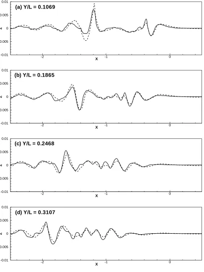
Figure 1 shows wave cuts for the 10.5 knot case. The correlation coefficients between experimental mea-surements and numerical predictions for parts (a) thru (d) of Figure 1 are 0.89, 0.91, 0.85, and 0.86, respec-tively. The solid and dashed lines respectively denote the experimental measurements and the numerical pre-dictions. The correlation gets poorer in the region where the grid spacing along the y-axis gets poorer. The short-est waves are not resolved by the numerical simulations. More grid resolution is required. Convergence studies are in progress.

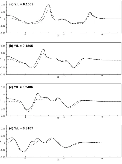
Figure 2 are 0.89, 0.92, 0.88, and 0.91, respectively. In general, the high Froude-number simulation is in slightly better agreement with the experimental measurements than the low Froude-number simulation, probably be-cause the waves are longer. However, both simulations would benefit from using higher resolution, especially near the bow and transom where there is wave breaking and flow separation.

5415 geometry

Experimental measurements of a DDG model 5415 have been performed at Froude numbersF r=0.2755 and 0.4136that correspond to equivalent full-scale speeds of 20 and 30 knots, respectively. The measurements include free-surface profiles on the ship hull, free-surface eleva-tions near the bow and stern using a whisker probe, and total drag. The length, beam, and draft of the model are respectively 5.72m, 0.388m, and 0.248m. The model-scale speeds are 4.01 and 6.02 knots. Details of the hull geometry, including the sinkage and trim, are provided by the Carderock Division (2005).

A three-dimensional numerical simulation using 800x192x192=29,491,200 grid points, 4x8x8=256 sub-domains, and 256 nodes has been performed on a Cray XT3. The length, width, depth, and height of the com-putational domain are respectively 3.0, 1.0, 1.0, 0.5 ship lengths (L). Grid stretching is employed in all directions. The smallest grid spacing is 0.0008L near the ship and mean waterline, and the largest grid spacing is 0.05L in the far field. For the high Froude-number case, this provides about 15 x 100 grid cells across the transom and 1340 grid cells per transverse wavelength (1.07L) where the grid spacing is fine and 20 grid cells where it is coarse. Initial transients are minimized by slowly ramping up the free-stream current. As before, the pe-riod of adjustment associated with this ramp up is 0.5 in non-dimensional units of time. For this simulation, the non-dimensional time step is t=0.0002. The numerical simulation runs 28001 time steps corresponding to 5.6 ship lengths. It requires 125 hours of wall-clock time.

Figure 4 compares NFA predictions to experimen-tal measurements for the flow near the bow. The free-surface profile measurements are denoted by spherical symbols along the ship hull. The ship hull is outlined in grey. Whisker-probe measurements are indicated by the small spherical symbols transverse to the ship. Due to the measuring technique, whisker-probe data provides an upper bound of the free-surface elevation. NFA pre-dictions of the free surface are denoted by the color con-tour. In general, the whisker-probe measurements agree well with the upper bound of the free-surface predictions. NFA correctly predicts the overturning of the bow wave and the resulting splash up slightly aft of the bow. At this resolution, the numerical simulations do not resolve the very thin sheets which characterize the run-up near

the bow. As a result, the NFA predictions are slightly lower than the maximum free-surface profile that has been measured.

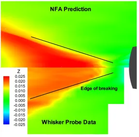
Figure 3 compares NFA predictions to whisker-probe measurements for the flow near the stern. The portion above the centerline of the ship represents NFA results while the portion below is based on experiments. Black lines mark the edges where spilling occurs. NFA accurately captures the flow separation from the transom stern and agreement between predictions and measure-ments is good overall. However, at this resolution some spilling along the edges of the rooster tail is not captured. As a result, the predicted rooster-tail amplitude directly astern of the transom is higher than measurements. Sim-ulations that resolve the breaking in this region may pro-vide the dissipation of energy that is necessary to reduce the wave amplitude in the rooster-tail region.

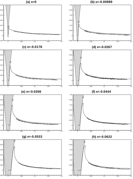
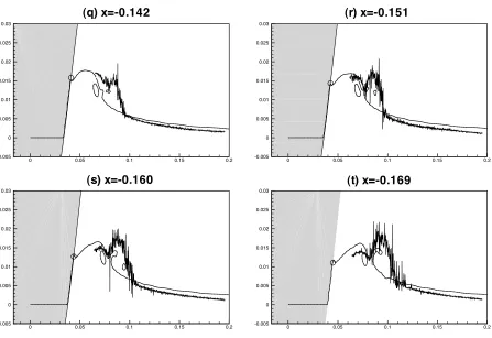
Figure 5 shows transverse cuts of the free-surface elevation near the bow. The cross section of the port side of the hull is outlined using a grey shade. Circular symbols denote the profile measurements along the side of the hull. Solid lines denote whisker-probe measure-ments. Dashed lines denote NFA predictions. Results are shown for various stations aft of the bow from (a) x=0 to (t) x=-0.169L, where L is the ship length. The figures show the overturning of the bow wave. The initial onset of air entrainment is evident in the NFA predictions. In addition, fragments of splash up are also captured. As expected, the whisker-probe measurements provide an upper envelope to the numerical predictions. This effect is illustrated in Figure 5k, where the bow wave is just beginning to overturn. For this station, there is a sud-den jump in the whisker-probe measurement that corre-sponds to the instrument measuring the top of the spray sheet. The envelop of the plunging event is captured well by the numerical simulations as illustrated in Figures 5k-o. Figures 5o & 5p show the initial stages of splash up. The results of the numerical simulation are not as ener-getic as the experiments. Higher resolution may help in this particular region. The entrainment of air is observed in Figure 5p-t. The splash up is resolved better by the numerical simulations in Figures 5s & 5t. However, the whisker-probe measurements are consistently lower than the numerical simulations in Figures 5q-t. This requires further study to find the source of the discrepancy.

Figure 6 shows the total resistance as a function of time. Time is normalized byLo/Uo, whereLo= 5.72m

an Euler code that does not directly predict skin-friction drag. Unlike potential-flow formulations, NFA does not require a correction for residuary resistance associated with the shedding of vorticity because Euler formula-tions account for base drag. The figure shows NFA re-sults converging to the steady-state resistance. We note that there are known long-time transients associated with a ship accelerating from rest to constant forward speed (Dommermuth, Sussman, Beck, T.O’Shea, Wyatt, Olson & MacNeice 2004).

Sphere geometry

Consider the motion of a heaving sphere that is mov-ing with forward speed. The purpose of this study is to build toward developing a capability that is suitable for forced-motion studies and seakeeping. The Froude number isF r = Uo/√gD = 0.5, whereD is the di-ameter of the sphere. The normalized didi-ameter of the sphere is D = 1. The amplitude of the heaving mo-tion is A = 0.25 and the frequency of oscillation is

ω = 2π(see Equation 33). Three grid resolutions are studied: 643 _{= 262,144, 128}3 _{= 2,097,152, and} 2563 _{= 16,777,216grid points. The length, width, and} height of the computational domain are 4. The smallest grid spacings for the coarse, medium, and fine grids are respectively 0.00412, 0.0206, and 0.0103. The time steps are respectively 0.0025, 0.00125, and 0.0006225.

Figure 7 shows the x-component of force acting on a sphere moving with forward speed, and Figure 8 shows the z-component. The forces are normalized by the dis-placement of the sphere, which is initially half immersed. The forces only include the portion of the pressure that is directed normal to the surface of the sphere. The ef-fects of skin friction are not included. First- and second-harmonic interactions are evident in both components of force. The second-harmonic interactions are particularly strong for the vertical component of force, probably due to wave breaking and collapse beneath the sphere.

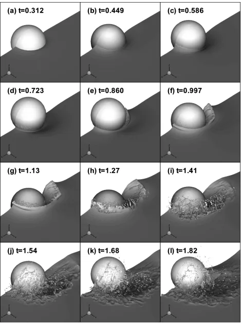
Figure 9 shows a time sequence of a heaving sphere moving with forward speed. The initial start-up stage is shown. A plunging breaker forms near the bow in Figure 9g. Upon breakup, the flow becomes very turbulent.

Conclusions

In terms of progress, it is interesting to consider the re-sults of research reported in earlier ONR symposiums. Dommermuth et al. (1998) study the flow near the bow of model 5415 using a variable-density, cartesian-grid for-mulation. A body force is used by Dommermuth et al. (1998) to impose the body boundary condition. The nu-merical results of Dommermuth et al. (1998) barely cap-ture the initial onset of wave overturning near the bow. Sussman & Dommermuth (2001) continue to develop

interface capturing methods. Once again, comparisons are shown to the bow flow of model 5415. The results do not show significant improvement over their earlier results. However, their calculations of the breakup of a turbulent spray sheet illustrate a novel application of interface-capturing methods. Dommermuth et al. (2004) use two methods to study the flow around model 5415, a vertical strut, and a bluff wedge. The first method uses free-slip conditions on the hull in combination with a hy-brid level-set and VOF interface-capturing method. In addition, adaptive mesh refinement (AMR) is used to im-prove grid resolution near the hull and free-surface inter-face. Their preliminary results illustrate the efficiency of AMR. The second method uses body-force and VOF formulations on a cartesian grid with no grid stretching. The results show more fine-scale detail than the earlier studies. The predicted free-surface elevations compare well with experiments, but the body-force method is too “sticky.” Based on these results, the present research uses free-slip boundary conditions to impose the body bound-ary condition to reduce stickiness. The VOF algorithm has been generalized to include free-slip conditions on the ship hull. The grid is stretched along the cartesian axes to improve grid resolution. Together, these new for-mulations enable the modeling of complex free-surface flows.

It is not possible to show all of the details in the cur-rent numerical predictions through the use of figures. In order to study the flow in even more detail, several ani-mations have been prepared at the flow visualization cen-ter at ERDC. The animations are accessible by contact-ing the authors. Animations are available for all the cases shown in this paper.

Acknowledgements

This research is supported by ONR under contract numbers N00014-04-C-0097. Dr. Patrick Purtell is the program manager. This work was supported in part by a grant of computer time from the DOD High Performance Computing Modernization Program (http://www.hpcmo.hpc.mil/). The numerical simula-tions have been performed on the Cray XT3 at the U.S. Army Engineering Research and Development Center and the Cray X1 at the Army High Performance Com-puting Research Center..

References

Carderock Division, Surface Ship Model 5415, Tech. rep., Naval Surface Warfare Center, 2005.

URL: http://www.dt.navy.mil/hyd/sur-shi-mod/

M., “An embedded boundary / volume of fluid method for free-surface flows in irregular geometries,” Proceedings of FEDSM99, 3rd ASME/JSME Joint Fluids Engineering Conference, San Francisco, CA., 1999, pp. 0–0.

Dommermuth, D., “The initialization of vortical free-surface flows,” J. Fluids Eng., Vol. 116, 1994, pp. 95–102.

Dommermuth, D., Innis, G., Luth, T., Novikov, E., Schlageter, E., & Talcott, J., “Numerical simulation of bow waves,” Proceedings of the 22nd Symposium on Naval Hydrodynamics, Washington, D.C., 1998, pp. 508–521.

Dommermuth, D. G., “The initialization of nonlinear waves using an adjustment scheme,” Wave Motion, Vol. 32, 2000, pp. 307–317.

Dommermuth, D. G., Sussman, M., Beck, R. F., T.O’Shea, T., Wyatt, D. C., Olson, K., & MacNeice, P., “The numerical simulation of ship waves using cartesian-grid methods with adaptive mesh refinement,” Proceedings of the 25th Symposium on Naval Hydrodynamics, St. John’s, Newfoundland and Labrador, Canada, 2004, pp. 0–0.

Gueyffier, D., Li, J., Nadim, A., Scardovelli, R., & Zaleski, S., “Volume-of-fluid interface tracking with smoothed surface stress methods for three-dimensional flows,” J. Comp. Phys., Vol. 152, 1999, pp. 423–456.

Knupp, P. M. & Steinerg, S., Fundamentals of grid generation, CRC Press, Inc., 1993.

Leonard, B., “Bounded higher-order upwind multidimensional finite-volume convection-diffusion algorithms,” W. Minkowycz & E. Sparrow, eds., Advances in Numerical Heat Transfer, Taylor and Francis, Washington, D.C., 1997, pp. 1–57.

Mampaey, F. & Xu, Z.-A., “Simulation and experimental validation of mould filling,” Modeling of Casting, Welding and Advanced Solidification Processes VII, London, England, 1995, pp. 10–12.

Orlanski, I., “A simple boundary condition for unbounded hyperbolic flows,” J. Comp. Phys., Vol. 21, 1976, pp. 251–269.

Pilliod, J. & Puckett, E., Second-Order Accurate Volume-of-Fluid Algorithms for Tracking Material Interfaces, Technical Report LBNL–40744, Lawrence Berkeley National Laboratory, 1997.

Puckett, E., Almgren, A., Bell, J., Marcus, D., & Rider, W., “A second-order projection method for tracking fluid interfaces in variable density incompressible flows,” J. Comp. Physics, Vol. 130, 1997, pp. 269–282.

Repetto, R. A., Computation of turbulent free-surface flows around ships and floating bodies, Ph.D. thesis, Technischen Universit¨at Hamburg-Harburg, 2000.

Rider, W., Kothe, D., Mosso, S., Cerutti, J., & Hochstein, J.,

“Accurate solution algorithms for incompressible multiphase flows,” AIAA paper 95–0699. Sussman, M., “A second order coupled level set and

volume-of-fluid method for computing growth and collapse of vapor bubbles,” J. Comp. Phys., Vol. 187, 2003a, pp. 110–136.

Sussman, M. & Dommermuth, D., “The numerical simulation of ship waves using cartesian-grid methods,”

Proceedings of the 23rd Symposium on Naval Ship Hydrodynamics, Nantes, France, 2001, pp. 762–779. Wilson, W., Fu, T., Pence, A., & Gorski, J., “The measured and

X

Z

-2 -1 0

-0.01 -0.005 0 0.005 0.01

(b) Y/L = 0.1865

X

Z

-2 -1 0

-0.01 -0.005 0 0.005 0.01

(d) Y/L = 0.3107

X

Z

-2 -1 0

-0.01 -0.005 0 0.005 0.01

(c) Y/L = 0.2468

X

Z

-2 -1 0

-0.01 -0.005 0 0.005 0.01

(a) Y/L = 0.1069

X

Z

-2 -1 0

-0.02 -0.01 0 0.01

0.02

(b) Y/L = 0.1865

X

Z

-2 -1 0

-0.02 -0.01 0 0.01

0.02

(d) Y/L = 0.3107

X

Z

-2 -1 0

-0.02 -0.01 0 0.01

0.02

(c) Y/L = 0.2486

X

Z

-2 -1 0

-0.02 -0.01 0 0.01

0.02

(a) Y/L = 0.1069

Figure 3: Model 5415 bow view.

0 0.05 0.1 0.15 0.2 -0.005

0 0.005 0.01 0.015 0.02 0.025 0.03

(a) x=0

0 0.05 0.1 0.15 0.2

-0.005 0 0.005 0.01 0.015 0.02 0.025 0.03

(a) x=0

0 0.05 0.1 0.15 0.2

-0.005 0 0.005 0.01 0.015 0.02 0.025 0.03

(b) x=-0.00889

0 0.05 0.1 0.15 0.2

-0.005 0 0.005 0.01 0.015 0.02 0.025 0.03

(c) x=-0.0178

0 0.05 0.1 0.15 0.2

-0.005 0 0.005 0.01 0.015 0.02 0.025 0.03

(d) x=-0.0267

0 0.05 0.1 0.15 0.2

-0.005 0 0.005 0.01 0.015 0.02 0.025 0.03

(e) x=-0.0356

0 0.05 0.1 0.15 0.2

-0.005 0 0.005 0.01 0.015 0.02 0.025 0.03

(f) x=-0.0444

0 0.05 0.1 0.15 0.2

-0.005 0 0.005 0.01 0.015 0.02 0.025 0.03

(g) x=-0.0533

0 0.05 0.1 0.15 0.2

-0.005 0 0.005 0.01 0.015 0.02 0.025 0.03

(h) x=-0.0622

0 0.05 0.1 0.15 0.2 -0.005

0 0.005 0.01 0.015 0.02 0.025 0.03

(a) x=0

0 0.05 0.1 0.15 0.2

-0.005 0 0.005 0.01 0.015 0.02 0.025 0.03

(i) x=-0.0711

0 0.05 0.1 0.15 0.2

-0.005 0 0.005 0.01 0.015 0.02 0.025 0.03

(j) x=-0.0800

0 0.05 0.1 0.15 0.2

-0.005 0 0.005 0.01 0.015 0.02 0.025 0.03

(k) x=-0.0889

0 0.05 0.1 0.15 0.2

-0.005 0 0.005 0.01 0.015 0.02 0.025 0.03

(l) x=-0.0978

0 0.05 0.1 0.15 0.2

-0.005 0 0.005 0.01 0.015 0.02 0.025 0.03

(m) x=-0.107

0 0.05 0.1 0.15 0.2

-0.005 0 0.005 0.01 0.015 0.02 0.025 0.03

(n) x=-0.116

0 0.05 0.1 0.15 0.2

-0.005 0 0.005 0.01 0.015 0.02 0.025 0.03

(o) x=-0.124

0 0.05 0.1 0.15 0.2

-0.005 0 0.005 0.01 0.015 0.02 0.025 0.03

(p) x=-0.133

0 0.05 0.1 0.15 0.2 -0.005

0 0.005 0.01 0.015 0.02 0.025 0.03

(a) x=0

0 0.05 0.1 0.15 0.2

-0.005 0 0.005 0.01 0.015 0.02 0.025 0.03

(q) x=-0.142

0 0.05 0.1 0.15 0.2

-0.005 0 0.005 0.01 0.015 0.02 0.025 0.03

(r) x=-0.151

0 0.05 0.1 0.15 0.2

-0.005 0 0.005 0.01 0.015 0.02 0.025 0.03

(s) x=-0.160

0 0.05 0.1 0.15 0.2

-0.005 0 0.005 0.01 0.015 0.02 0.025 0.03

(t) x=-0.169

Figure 5: Model 5415 transverse wave cuts, continued

Time

Fo

rc

e

X

(k

g

)

0 1 2 3 4 5 6

-30 -25 -20 -15 -10 -5 0

NFA Experiment

Time

XF

o

rc

e

0 1 2 3 4 5

-0.8 -0.6 -0.4 -0.2 0 0.2 0.4 0.6 0.8

Fine Medium Coarse

Figure 7: X-component of force acting on a heaving sphere moving with forward speed.

Time

ZF

o

rc

e

0 0.5 1 1.5 2 2.5 3 3.5 4 4.5 5

0 0.2 0.4 0.6 0.8 1 1.2 1.4 1.6 1.8 2

Fine Medium Coarse