FIR GEM: A SOE DSGE Model for fiscal policy analysis in Ireland ESRI WP620, March 2019

FIR-GEM: A SOE-DSGE Model for fiscal policy analysis in Ireland

Petros Varthalitis

Abstract: This paper presents FIR-GEM: Fiscal IRish General Equilibrium Model. FIR-GEM is a small open economy DSGE model designed as fiscal toolkit for fiscal policy analysis in Ireland. To illustrate the model's potential for fiscal policy analysis, we conduct three types of experiments. First, we analyse the fiscal transmission mechanism through which Irish fiscal policy affects the Irish economy. Second, we compute fiscal multipliers for the main tax-spending instruments, namely government consumption, public investment, public wage bill, public transfers, consumption, labour and capital tax. We focus on a fiscal policy stimulus that is either implemented through spending increases or tax cuts. Third, we perform robustness analysis on key structural characteristics that can affect quantitatively the size of fiscal multipliers. We find that the size of fiscal multipliers in the Irish economy heavily depends on its degree of openness, the method of fiscal financing employed, the elasticity of the sovereign risk premia to Irish debt dynamics and the flexibility of Irish labour and product markets.

Keywords: Fiscal policy, DSGE, Ireland, Openness.

JEL classifications: E62, F41, F42.

Acknowledgements: FIR-GEM was developed as part of the joint research programme 'Macroeconomy, Taxation and Banking' between the ESRI, the Department of Finance and Revenue Commisioners and I am grateful for helpful comments of the programme steering committee. I would like to especially thank Alan Barrett, Martina Lawless, Campbell Leith, Kieran McQuinn, Dimitris Papageorgiou and Apostolis Philippopoulos for many helpful suggestions and comments. I would also like to thank Adele Bergin, Abian Garcia-Rodriguez, Stelios Gogos, Ilias Kostarakos, Conor O'Toole and participants at the Quarterly Macro Meet up at the ESRI for useful comments. The views presented in this paper are those of the author and do not represent the official views of the ESRI, the Department of Finance and Revenue Commissioners. Any remaining errors are my own.

a. Economic and Social Research Institute, Economic Analysis, Whitaker Square, Sir John Rogerson's Quay, Dublin 2,. Ireland. Email: petros.varthalitis@esri.ie

ESRI working papers represent un-refereed work-in-progress by researchers who are solely responsible for the content

Working Paper No.

6

20

1

Introduction

FIR-GEM: Fiscal IRish General Equilibrium Model is a small open economy dynamic stochastic general

equilibrium model (SOE-DSGE) that attempts to capture the main features of the Irish economy. The primary

aim of FIR-GEM is to serve as a …scal policy toolkit for …scal policy analysis in Ireland. The present model

belongs to the class of medium-scale DSGE models that are widely used in policy institutions1_{. These models}

are based on microeconomic foundations and economic agent’s intertemporal choice. The general equilibrium

framework captures the interaction between policy actions and private agent’s economic behaviour. These

features are vital for …scal policy analysis. Fiscal policymaking can utilize a rich menu of tax and spending

instruments that could result in a wide range of macroeconomic outcomes. Fiscal actions do not only a¤ect

private agents’current economic decisions but their economic behaviour over time (intertemporal choices) by

in‡uencing their expectations about future …scal policy. This makes …scal policy analysis a complex task (see

Leeper (2010)). To evaluate and rank alternative …scal policies, research economists should take into account

an explicit analysis of the structure of the economy, private agent’s expectations and the dynamic adjustment

of their economic behaviour to those …scal policies2.

In addition, any macroeconomic and …scal policy analysis should take into account the speci…c structure

of the Irish economy3_{. In the next paragraphs, we summarize some structural characteristics of the Irish}

economy that the present model is designed to capture.

First, a key structural characteristic of Ireland is its exceptional degree of openness4_{. Ireland’s openness}

is re‡ected in a number of key macroeconomic aggregates. In particular, the larger size of the Irish tradable

sector5 _{vis-à-vis the non-tradable sector. For example, the ratio of the value added in the tradable sector}

to the value added in both sectors averages 59% over the period 2001 to 2014. Moreover, the Irish tradable

1_{For example European Commission DG ECFIN uses the Quest III model, see Ratto, Roeger, and in ’t Veld (2009) and the}

Global Multi-Country Model (GM), see Albonico et al. (2017). The ECB uses the New Area Wide Model (NAWM), see Warne, Coenen, and Christo¤el (2008) and Coenen et al. (2018). While several european countries have developped DSGE models, e.g. REMS, see Bosca et al. (2010) , and FiMOD for Spain, see Stahler and Thomas (2012), BoGGEM for Greece, see Papageorgiou (2014), GEAR for Germany see Gadatsch et al. (2015), AINO 2.0 see Kilponen et al. (2016) and many others.

2_{For a thorough discussion on the current state and role of DSGE models in policymaking see Gurkaynak and Tille (2017),}

Reis (2017) and Christiano, Eichenbaum, and Trabandt (2018).

3_{Papers focusing on various aspects of the Irish economy over time include FitzGerald (2000), Honohan and Walsh (2002),}

Lane (2009), Whelan (2014), Fitzgerald (2018).

4_{On the role of openness see CESifo (2014), Fitzgerald (2014) and McQuinn and Varthalitis (2018).}

5_{The Irish tradable sector is dominated by foreign a¢ liated …rms (Multinational Enterpirses), this is re‡ected in the sector}

sector is highly export-oriented6, for example the exports to GDP ratio averages 96% between 2001 and 20147.

Domestic consumption and production heavily rely on imports while the Irish trade surplus averages 14% as a

share of GDP over the period 2001 to 2014. In order to capture these characteristics of the Irish economy, we

incorporate two sectors of domestic private production, i.e. we distinguish between the tradable and the

non-tradable sectors. The factors of production are sector speci…c while sectoral reallocation entails production

costs (as in Uribe and Schmitt-Grohe (2017)).

Second, Ireland is modelled as a small open economy participating in a currency union (Eurozone). This

implies that households and government can participate in global …nancial and capital markets but their

behaviour cannot in‡uence the world interest rate8. As a result, we follow Schmitt-Grohe and Uribe (2003) and

assume that the nominal interest rate faced by domestic residents in the world …nancial markets is an increasing

function of the deviation of the Irish public debt to GDP ratio from a threshold level (for similar modelling

see Garcia-Cicco, Pancrazi, and Uribe (2010) and Philippopoulos, Varthalitis, and Vassilatos (2017)). This

assumption is empirically relevant and has non trivial implications for the e¢ cacy of …scal policy. Being a

member of the Eurozone implies the loss of monetary independence and a …xed nominal exchange rate regime

for the Irish economy. Thus the only macroeconomic policy tool available is …scal policy.

Third, Irish …scal policy over the period 2001 to 2014 is characterized by relatively low automatic

stabiliz-ers.9 Indicatively, government expenditures and tax revenues as shares of GDP are among the lowest within

Eurozone countries, they amount to 38% and 34%10 _{of GDP between 2001 and 2014.}11 _{The present model}

incorporates a rich menu of …scal policy instruments. In particular, the Government has four spending

instru-ments at its disposal, namely government consumption, public investment, public wages and agent-speci…c

public transfers and three tax instruments, namely consumption, labour and capital taxes. In addition, the

Government can issue domestic and foreign public debt (along with taxes levied on households) which are

6_{For more details on the composition of the Irish tradable sector see Barry and Bergin (2012) and Barry and Bergin (2018).}

7_{Although this …gure reduces to 52% in value added terms for 2001-2011, it still highlights the importance of exports in the}

Irish economy.

8_{As is well known, a small open economy with an exogenous world interest rate induces non-stationary dynamics.}

9_{For e.g. Kostarakos and Varthalitis (2019) compare e¤ective tax rates in Ireland with Eurozone average and …nd that Irish}

ETRs rank amongst the lowest.

1 0_{We also express Irish …scal aggregates as GNI shares, since GDP and GNI di¤er by 15% on average over 2001-2014. Although}

the gap between Eurozone averages and Ireland closes, Irish …scal aggregates remain amongst the lowest within Eurozone countries. For example government expenditures and tax revenues amount to 45% and 39% in Ireland while Eurozone averages are 48% and 45% respectively.

1 1_{Ireland recently implemented a front-loaded …scal consolidation package via mostly expenditure cuts (for more details on the}

used to …nance public expenditures. We adopt a rule-like approach to policy in that …scal policy is conducted

via simple and implementable …scal policy rules.12 Here, all the main tax-spending instruments are allowed

to react to the public debt to GDP ratio and the level of the de…cit so as to ensure …scal sustainability.13 _In

addition, a …rm in the public sector utilizes goods purchased from the private sector, public employment and

public capital to produce a good that provides both welfare-enhancing and productivity-enhancing services.14

Fourth, we incorporate in the model several features that quantitatitavely matter for the …scal transmission

mechanism and are empirically relevant (see e.g. in Zubairy (2014) and in Leeper, Traum, and Walker (2017)).

Namely households with non-Ricardian behaviour (as in e.g. Gali, Lopez-Salido, and Valles (2007)), real

frictions and nominal rigidities, while, we allow for complementarity/subsitutability between private/public

consumption and productivity-enhancing public goods.

We calibrate the model using Irish annual data over the period 2001-201415_{. To illustrate the model’s}

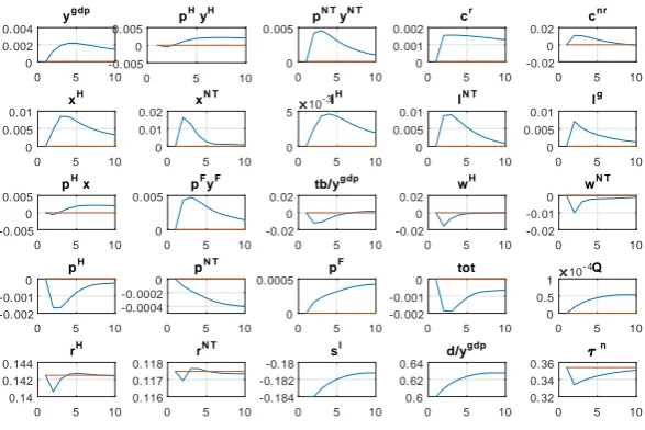
ability to assess …scal policy, we conduct three types of simulations. First, we use the model to examine the

…scal transmission mechanism through which Irish …scal policy a¤ects the Irish economy. Second, we compute

…scal multipliers for the main tax-spending instruments, namely government consumption, public investment,

public wage bill, public transfers, consumption, labour and capital tax. We focus on a …scal stimulus policy

that is either implemented through spending increases or tax cuts. Third, we perform robustness analysis on

structural characteristics that can a¤ect qualitatively and quantitatively the size of …scal multipliers in the

Irish case. These include the degree of openness, alternative …scal …nancing methods, the sensitivity of the

international nominal rate at which Ireland borrows from the rest of the world to Irish public debt dynamics,

complementarity/subsitutability of public and private consumption, ‡exibility of the Irish labour and product

markets.

The main results are as follows: …rst Irish …scal multipliers are expected to be smaller in magnitude than

most EU countries due to the degree of openness of the domestic economy and the large in‡uence of the

tradable sector. Second …scal policy a¤ects the composition of aggregate output. The …scal stimulus works

1 2_{In Schmitt-Grohe and Uribe (2005) and (2007) “simple” and “implementable” means that policy can easily and e¤ectively}

be communicated to the public; that is policy instruments react to a small number of easily observed macroeconomic indicators.

1 3_{Most European countries set their policy by following some type of …scal rules so this is an empirically relevant assumption}

(see European Commission 2012).

1 4_{For DSGE models that incorporate a public production function see e.g. Forni et al. (2010), Papageorgiou (2014), Economides}

et al. (2013) and (2017).

1 5_{We focus over the period 2001-2014 since there are well documented problems with Irish national accounts after 2014 for}

solely through the non-tradable sector while the tradable sector remains una¤ected or contracts in size. The

latter is crucial in the Irish case where the tradable sector is signi…cantly larger than the non-tradable sector.

Third a …scal stimulus via spending produces more output than a stimulus via tax cuts in the short run;

that is spending multipliers are consistently larger than tax multipliers. Fourth, in terms of the e¤ect on

GDP in the …rst year, the most e¤ective Irish …scal instruments are as follows: public investment, government

consumption, consumption taxes, capital taxes, public transfers, public wages and, …nally, labour taxes. Fifth,

a …scal expansion via spending is expected to have a negative e¤ect on the competitiveness of the domestic

economy. Our results show a deterioration of the Irish external balance in the early years of the stimulus era;

that is the …scal stimulus is likely to crowd out exports and at the same time crowd in imports. Sixth, income

tax cuts induce a smaller e¤ect on the Irish external balance. Capital and labour tax cuts are expected to

reduce production costs and prices in Ireland vis-à-vis the rest of the world leading to an improvement in

the competitiveness of the Irish economy. As such, a …scal expansion via tax cuts induces supply-side e¤ects

that take time to materialize (i.e. multipliers are smaller in the short run) but their e¤ects are long lasting.

Seventh, the method of …scal …nancing is crucial for the e¢ cacy of a …scal stimulus. A spending stimulus

…nanced via tax increases mitigates the positive e¤ect on GDP.

The remainder of the paper is organized as follows. Section 2 reviews the literature. Section 3 solves the

model. Section 4 develops the calibration strategy and presents the steady state solution. Section 5 analyses

the …scal transmission mechanism of the model. Section 6 quanti…es …scal multipliers in the Irish case. Section

7 conducts a robustness analysis, while Section 8 concludes and discusses possible avenues for future research.

An appendix presents details of the model.

2

Related Literature

This paper contributes to the literature on medium scale SOE-DSGE models for …scal policy analysis in

policy institutions. Our work emphasizes the role played by the degree of openness in the …scal transmission

mechanism in Ireland and quanti…es …scal multipliers for the main tax-spending Irish …scal instruments. There

are three papers that quantify …scal multpliers for Ireland, in particular, Clancy, Jacquinot, and Lozej (2016)

model (EAGLE), Bergin and Garcia-Rodriguez (2019) use the ESRI COSMO large-scale macroeconometric

model16 to compute …scal multipliers for tax-spending Irish …scal instruments and Ivory, Casey, and Conroy

(2019) estimate spending multipliers using a suite of VAR-type models. To the best of our knowledge this is the

…rst paper that quanti…es all the main tax-spending multipliers for Ireland using a medium scale SOE-DSGE

model with a rich …scal sector, analyses the associated …scal transmission mechanism, provides an Irish …scal

instrument ranking with respect to their e¤ect in the Irish GDP and computes the e¤ects of …scal policy on

the composition of aggregate output and the competitiveness of the Irish economy.

DSGE models for Ireland17 include EIRE Mod, see Clancy and Merola (2016b), which however does not

incorporate an explicit …scal sector. Klein and Ventura (2018) develop a growth model for Ireland to study

the Ireland’s remarkable historical economic performance over 1980-2005 focusing on the role of …scal policy

while Ahearne, Kydland, and Wynne (2006) study Ireland’s depression episode over the period from 1973 to

1985.

This paper also contributes to the vast literature on …scal multipliers using DSGE models by quantifying

…scal multipliers in Ireland for the main tax-spending instruments18_{. For example, a similar study, Kilponen}

et al. (2015), compare tax-spending multipliers across fourteen countries in Europe. Our contribution also

lies in the …eld of …scal policy e¤ects on the trade balance and the composition of output, e.g. Monacelli and

Perotti (2008) and Monacelli and Perotti (2010) study the e¤ect of government spending on trade balance and

international relative prices19_.

1 6_{Bergin et al. (2017) develop a large-scale macroeconometric model estimated for Ireland in the spirit of NiGEM model}

developed by National Institute of Economic and Social Research.

1 7_{Clancy and Merola (2016a) and Lozej, Onorante, and Rannenberg (2018) develop SOE-DSGE models with …nancial frictions}

for Ireland focusing on macroprudential policies.

1 8_{The literature on …scal multipliers is volunimous for a detailed review see Battini et al. (2014) and the references therein. Some}

selective references are: Coenen, Straub, and Trabandt (2013) use a suite of DSGE models to compute multipliers, Leeper, Traum, and Walker (2017) use bayesian techniques to quantify the size of multipliers across di¤erent model speci…cations, Zubairy (2014) and Drautzburg and Uhlig (2015) use estimated models to compute …scal multipliers for U.S economy. Christiano, Eichenbaum, and Rebelo (2011) compute spending multipliers when the zero lower bound on the nominal interest rate binds, while Canzoneri, Collard, Dellas, and Diba (2016) …nd assymetric multipliers over the business cycle.

1 9_{Our results for Ireland with the remarkable degree of openness con…rm empirical studies, like Benetrix and Lane (2010) and}

3

A Small Open Economy Model

3.1

Informal description of the model

This section develops a small open economy dynamic general equilibrium model (SOE-DSGE) with a rich

…scal sector calibrated for Ireland. This model is designed as a …scal policy toolkit for Ireland, and thus

contains several key features seeking to resemble the structure of the Irish economy and, hence, be suitable

for …scal policy analysis. The model: (a) distinguishes between tradable and non-tradable production sectors;

(b) allows for sector-speci…city of factor inputs; (c) incorporates heterogeneous agents; (d) empirically relevant

nominal and real frictions; (e) debt-elastic interest rate; (f) delegated monetary policy (Ireland is a member of

a currency union) and independent national …scal authority and (g) it allows for an explicit …scal sector with

a rich menu of spending-tax …scal instruments, explicit …scal rules and a public production function.

This model belongs to the class of small open economies and thus incorporates several open economy

features. In particular, households and government can participate in international …nancial markets. To

ensure stationarity we assume that the international interest faced by domestic borrowers is debt elastic, as in

e.g. Schmitt-Grohe and Uribe (2003). Moreover, domestic economic agents can engage in international trade,

thus they can consume and invest in imports; while a share of domestic production is exported to the rest of

the world.

The model consists of three types of economic agents: households, …rms and a government. We

inco-prorate two type of households; …rst, forward-looking optimizing agents which have access to domestic and

international …nancial and capital markets while receiving dividends from domestic …rms. These households

are referred to as Ricardians or Savers. Second, …nancially constrained agents which do not have access to

…nancial and capital markets, that is they live hand to mouth and each period consume all of their after tax

disposable income. These households are referred to as non-Ricardians or non-Savers. The introduction of the

latter type of households in the model has non trivial e¤ects in the transmission mechanism of …scal policy

actions (see e.g. Gali, Lopez-Salido, and Valles (2007), Cespedes, Fornero, and Gali (2011) and Leeper, Traum,

and Walker (2017)). Non-Savers are relatively more prone to changes in government expenditures or/and taxes

since they cannot smooth out changes in their disposable income over time. Both type of households provide

they optimally allocate hours worked among these sectors. Both types of households pay consumption taxes

and receive household-speci…c public transfers, Ricardians pay labour and income taxes while non-Ricardians

pay only labour taxes.

The model incorporates private and public production. There are two stages of private production. In

the …nal stage, the …nal good, that is used for private and public consumption and investment, is produced.

There are two …rms namely a …nal good and a composite tradable good producer at this level. The …nal good

producer utilizes the composite tradable and the intermediate non-tradable good to produce the …nal good.

Similarly, the composite tradable good producer utilizes the home produced tradable good and the imported

good to produce the composite tradable good.

In the intermediate stage, the intermediate tradable and non-tradable bundles are produced. There are

Ni _{intermediate non-tradable …rms. Each non-tradable …rm indexed by i hires labour and rents physical}

capital from households to produce a di¤erentiated varietyi:A non-tradable distributor combines all varieties,

i= 1::Ni_{;into an intermediate non-tradable bundle. Similarly, there areN}j _{intermediate home tradable …rms.}

Each home tradable …rm indexed byj hires labour and rents physical capital from households to produce a

di¤erentiated varietyj: A tradable distributor combines all varieties, j = 1::Nj_{; into an intermediate home}

tradable bundle.

Firms in the public sector use goods purchased from the private sector, public employment and public

capital to produce a good that provides both utility-enhancing and productivity-enhancing services. The

associated public spending inputs are set exogenously by the government.

In terms of economic policy, Ireland is a member of the Eurozone thus we focus on a monetary policy

regime in which the nominal exchange rate is …xed and there is no monetary policy independence (this mimics

membership in a currency union). Fiscal policy is conducted via simple …scal policy rules.

3.2

Households

The economy is populated byNnumber of households. The population is comprised of two types of households,

Ricardian households (or Savers) indexed by the upperscriptr= 1::Nr _{and non-Ricardians (or Non Savers)}

3.2.1 Ricardian Households (Savers)

Preferences and Constraints There are Nr _{Ricardians/Savers indexed by the upperscript r = 1::N}r

t:

Each householdrmaximizes its expected discounted lifetime utility,Vr

0;in any given periodt :

V₀r E0

1

X

t=0

t

Ur ecr_t; l_tH;r; lN T ;r_t ; lP;r_t (1)

whereecrt crt+#gygt denotes composite consumption comprising ofcrt consumption of the …nal good (de…ned

in section 3.3.1 below) and y_tg consumption of public good per capita produced by a state …rm (de…ned

in section 3.4.2), #g > (<) 0, measures the degree of subsitutability (complementarity) between public and

private consumption, lH;r_t , lN T ;r_t and lP;r_t denote hours of work in the tradable, non-tradable and public

sectors20 _{respectively, 0< <1 is a subjective discount factor andE}

0 is the rational expectations operator

conditional on information at time0. Each household’s sequential budget constraint in periodt is given by

(in nominal terms):

Pt(1 + ct)crt+PtxH;rt +PtxN T ;rt +Ptbrt+StPtftr+ (ftr; f r)

= (1 n

t)Pt wHt l H;r

t +wN Tt l N T ;r t +wtPl

P;r

t + 1 kt Pt rtN T ;rk N T ;r t 1 +!

N T ;r t

+ 1 k_t Pt rtH;kk H;r t 1+!

H;r

t +Rt 1Pt 1brt 1+Qt 1StPt 1ftr 1 Pt l;rt

(2)

wherePtis the nominal price of the …nal good,lj;rt ; x j;r t ; k

j;r t ; r

j;k t ; w

j;r t and!

j;r

t are hours worked, gross

invest-ment, the beginning-of-period physical capital, the real return of capital, real wage rate and real pro…ts in sector

j=H; N T, wp_t denotes public wages,br

t andftrare the real value of the end-of-period domestic government

bonds and internationally traded assets (the latter is expressed in foreign currency) respectively21_,S

t is the

nominal exchange rate de…ned as the domestic currency price of one unit of foreign currency,Rt 1; Qt 1 1

denote the gross nominal return of domestic government bonds and international assets between t 1 and

t respectively; ct; nt; kt are consumption, labour and capital tax rates respectively, l;rt is public transfers

2 0_{Our modelling implies that each household is comprised of many members which can be employed in all three sectors.}

Then, each household allocates its members to each sector by maximizing its lifetime utility, for similar modelling see Uribe and Schmitt-Grohe (2017). See Ardagna (2001), Forni, Gerali, and Pisani (2010), Economides, Papageorgiou, Philippopoulos, and Vassilatos (2013) and Papageorgiou (2014), Economides, Papageorgiou, and Philippopoulos (2017) for models which include public employment.

2 1_{For simplicity and notational convenience and without loss of generality, all quantities and relative prices will be expressed}

targeted to Ricardian householdr. Finally, borrowing on the international market entails an adjustment cost

(:). The laws of motion for physical capital in tradable and non-tradable sectors are given by:

kH;r_t = 1 H kH;r_{t 1}+xH;r_t H kH;r_t ; kH;r_{t 1} (3)

k_tN T ;r= 1 N T kN T ;r_{t 1} +xN T ;r_t N T kN T ;r_t ; k_tN T ;r₁ (4)

where H and N T; H_(:)and N T_{(:)are sector speci…c depreciation rates and adjustment costs respectively.}

Functional forms of the period utility and the adjustment costs are speci…ed in Appendix G.

A key element of the Irish macroeconomic structure is the presence of two distinct sectors of production,

i.e. the tradable and non-tradable sector. Both have di¤erent structural characteristics. We allow for sector

speci…city by including features that aim to slow down the sectoral re-allocation of factors of production,

i.e. labour and physical capital (as in e.g. Uribe and Schmitt-Grohe (2017)). To do this, we, …rst, allow

for imperfect substitutability of labour across di¤erent sectors by introducing sector-speci…c hours worked as

separate arguments in the utility function. Second, we allow for sector-speci…c depreciation rates and capital

adjustment costs in the associated laws of motion (3) and (4). Both elements imply that factor movements

among sectors entails costs; the magnitude of these costs are calibrated to re‡ect the relevant Irish data.

Choice of allocations Each householdrmaximizes its lifetime utility (1) in any given periodtby choosing

purchases of the …nal consumption good,cr

t; hours of work in the tradable,l H;r

t ; non-tradable sector, l N T ;r t ,

and public sector,lP;r_t ;the end-of-period physical capital stocks,k_tH;r;andk_tN T ;r; the end-of-period holdings

of domestic government bond,br

t; and international traded assets expressed in foreign currency,ftr; subject

to the constraint (2) (in which we incorporate constraints (3) and (4)). The Lagrange multiplier associated

with constraint (2) is r_t . The …rst-order conditions with respect tocr_t; lH;r_t ; l_tN T ;r; lP;r_t ; k_tH;r; k_tN T ;r; br_t andf_tr

are given by:

@Ur t

@cr t

@Ur t

@l_tH;r =

r

t(1 nt)wHt (6)

@Ur t

@lN T ;r_t =

r

t(1 nt)wN Tt (7)

@U_tr @lP;r_t =

r

t(1 nt)wPt (8)

r t 1 +

@ (kH t ;kHt 1)

@kH

t =

E0 rt+1 1

H

+ 1 k

t+1 r

H;k t+1

@ (kHt+1;k

H t )

@kH t

(9)

r t 1 +

@ N T_(kN T t ;kN Tt 1)

@kN T

t =

E0 rt+1 1 N T + 1 kt+1 r

N T ;k t+1

@ N T(kN Tt+1;k

N T t )

@kN T t

(10)

r

t =E0 rt+1Rt

Pt 1 Pt

(11)

r t

StPt

Pt +

(ftr;f r

)

@f r

t =

E0 Qt+1 rt+1

St+1Pt+1

Pt+1

P_t P_t+1

(12)

3.2.2 Non-Ricardian Households (Non-savers)

In line with the empirical evidence see e.g. in Gali, Lopez-Salido, and Valles (2007), Cespedes, Fornero,

and Gali (2011) and Leeper, Traum, and Walker (2017), we incorporate a fraction of …nancially constrained

households which we refer to as non-Ricardian households or non-Savers.

Preferences and Constraints Each non-Ricardian household nrhas the same preferences as Ricardian

households and choosescnr t ; l

T ;nr t ; l

N T ;nr t andl

P;nr

t to maximize its expected discounted lifetime utility,V0nr:

V₀nr E0

1

X

t=0

t_{U ec}nr t ; l

H;nr t ; l

N T ;nr t ; l

P;nr

t (13)

subject to the sequential budget constraint in periodt(in nominal terms):

(1 + ct)Ptcnrt = (1 nt)Pt wHt ltH;nr+wN Tt lN T ;nrt +wPtlP;nrt Pt l;nrt (14)

public sectors; but they have no access to capital or/and …nancial markets. In other words, they live

hand-to-mouth and consume their after tax labour income plus targeted government lump-sum transfers,Pt l;nrt <0:

Choice of allocations Each household nr maximizes its lifetime utility (13) in any given period t by

choosing purchases of the …nal good,cnr

t ;hours of work in the tradable,l H;nr

t ;non-tradable sector,l N T ;nr t ;and

public sector,lP;nr_t subject to the constraint (14). The Lagrange multiplier associated with constraint (14) is

nr

t . The …rst-order conditions with respect tocnrt ; l H;nr t ; l

N T ;nr t ; l

P;nr t are:

@U_tnr @cnr t

= nr_t (1 + c_t) (15)

@Unr t

@lH;nr_t =

nr

t (1 nt)wtH (16)

@U_tnr @l_tN T ;nr =

nr

t (1 nt)wtN T (17)

@Unr t

@lP;nr_t =

nr

t (1 nt)wPt (18)

3.3

Firms

There are two stages of private production. In the …nal stage, the …nal good that is used for private and public

consumption and investment is produced. There are two …rms namely a …nal good and a composite tradable

good producer (the associated problems are solved in sections 3.3.1 and 3.3.2). The …nal good producer utilizes

the composite tradable and the single intermediate non-tradable good to produce the …nal good. Similarly,

the composite tradable good producer utilizes the home produced tradable good and the imported good to

produce the composite tradable good.

In the intermediate stage, the intermediate non-tradable and tradable bundles are produced (the associated

problems are solved in sections 3.3.3 and 3.3.4). There are Ni _{intermediate tradable …rms, each}

non-tradable …rm indexed byi hires labour and rents physical capital from households to produce a di¤erianted

variety i: A non-tradable distributor combines all varieties, i = 1::Ni; into an intermediate non-tradable

bundle. Similarly, there areNj _{intermediate home tradable …rms, each home tradable …rm indexed byj hires}

combines all varieties,j= 1::Nj; into an intermediate home tradable bundle.

3.3.1 Final good producer

In this section, we solve the problem of the …nal good producer in per capita terms22_{. The …nal good is}

produced using a non-tradable good,yN T

t , and a composite tradable good,yTt;via a CES technology:

yt= (v)

1 ytT

1

+ (1 v)1 ytN T

1 1

(19)

where is the intratemporal elasticity of substitution between the composite tradable good and the

non-tradable good, andv₂(0;1]is a share parameter governing the share of the composite tradable input and the

non-tradable input in the production of the …nal good. The producer of the …nal good behaves competitively

and maximizes its pro…ts given by:

Ptyt PtTytT PtN TyN Tt

demand functions for the composite tradable good and the non-tradable good are given by:

@yt

@yT t

=P

T t

Pt

(20)

@yt

@yN T t

=P

N T t

Pt

(21)

Combining (20) and (21) yields:

y_tT = v

1 v

PT t

PN T t

yN T_t (22)

while the associated price index is:

Pt=

h

v P_tT 1 + (1 v) P_tN T 1

i 1 1

(23)

2 2_{Notice that throughout the paper small case letters denote per capita (…rm) quantitities,zt} Zt

N;while capital case letters

3.3.2 Composite tradable good producer

The composite tradable good is produced using the domestic absorption of the home tradable good,yH;d_t , and

an imported good,yF

t;via a CES technology:

y_tT =

"

vH 1

H

y_tH;d

H ₁ H

+ 1 vH

1

H

yF_t

H ₁ H

# H H 1

(24)

where His the intratemporal elasticity of subsitution between the domestic absorption of home tradable good

and the imported good andvH _{2(0;1]denotes a share parameter that determines the share of the domestic}

absortpion of the home tradable good vis-à-vis the imported good. Also it determines implicitly, the share of

the home tradable good which is exported to the rest of the world. This parameter can capture key features

of the Irish economy like the export orientation of home tradable production and the share of imported inputs

in the production of the composite and the …nal good. The producer of the composite tradable good behaves

competitively and maximizes its pro…ts given by:

PtTytT PtHyHt PtFyFt

demand functions for the domestic tradable good and imported good are given by:

@yT t

@yH t

=P

H t

PT t

(25)

@yt

@yN T t

=P

F t

PT t

(26)

Combining (25) and (26) yields:

yH;d_t = v

H

1 vH

PH t

PF t

H

yF_t (27)

while the associated price index is:

P_tT = vH P_tH 1

H

+ 1 vH P_tF 1

H

1 1 H

where

PtF =StPt (29)

In the next two subsections we explain how the tradable and non-tradable goods are produced.

3.3.3 Non-tradable sector

Non-tradable good distributor A non-tradable good distributor combines varieties, i = 1::Ni; of the

intermediate non-tradable goods, yN T ;it , into a composite non-tradable good, YtN T; using a Dixit-Stiglitz

aggregator:

Y_tN T

0 @

Ni X

i=1 y_tN T ;i

"N T 1

"N T 1 A

"N T "N T 1

whereY_tN T andyN T_t YtN T

N denote aggregate and per capita quantity respectively,"

N T _{>0is the elasticity}

of substitution across goods i. The non-tradable good distributor maximizes its pro…ts by choosing, YtN T;

while taking prices,PN T t andP

N T ;i

t ;as given:

P_tN TY_tN T

Ni

X

i=1

P_tN T ;iy_tN T ;i

The optimality condition yields a downward slopping demand function for each intermediate good of variety

i:

yN T ;i_t =

"

PtN T ;i

PN T t

# "N T

yN T_t

where the associated price index isPN T t

PNi i=1 P

N T ;i t

1 "N T

1 1 "N T

:

Intermediate non-tradable goods …rms There areNi_{intermediate non-tradable good …rms indexed by}

the upperscripti:Each intermediate non-tradable good …rmisupplies varietyiby solving a two-step problem.

First, intermediate …rmiminimizes its cost by choosing its factor inputskN T ;i_{t 1} andlN T ;it :

y_tN T ;i = min

fk_tN T ;i₁ ;lN T ;it g n

Ptrktk N T ;i

t 1 +PtwtN Tl N T ;i t

o

yN T ;it =AN Tt fygtg{

N T

1 _kN T ;i

t 1

aN T

ltN T ;i

1 aN T {N T2

(30)

Each intermediate non-tradable good …rm i produces a di¤erentiated product i utilising as inputs, yg_t; per

…rm public good (see section 3.4.2) which is used as an intermediate input in the private production,kN T ;i_{t 1} ;

physical capital rented from households in fully competitive capital markets and labour services rented from

households,l_tN T ;i;in fully competitive labour markets.23 _AN T

t is a scale parameter that measures productivity

in the non-tradable sector. {N T

1 > 0 is a parameter that determines the share of the public good as an

intermediate productive input,{2N T 2[0;1]determines the share of private productive inputs.24 WhileaN T

and1 aN T are structural parameters related to capital and labour income share in the non-tradable sector.

The …rst order conditions are given by (where N T ;i_t is the Lagrange multiplier associated with (30)):

Ptrkt = N T ;i

t aN T{N T2 yN T ;i_t

kN T ;i_{t 1} (31)

PtwtN T = N T ;i

t 1 aN T {2N T y_tN T ;i

lN T ;i_t (32)

Plugging the conditional factor demands into the nominal cost function we get the minimum nominal cost

function for any given level of production, yN T ;i_t :It can be shown that the associated Lagrange multiplier

is equal to the nominal marginal cost N T ;i_t = @ (y

N T ;i

t )

@ytN T ;i

:Nominal pro…ts of …rmi can be written as:

Pt!N T ;it =P N T ;i t y

N T ;i

t Ptrtkk N T ;i

t 1 PtwtN Tl N T ;i t

N T

2

P_tN T ;i P_tN T ;i₁ 1

!2

P_tN TyN T_t (33)

In the second step, each …rmichooses its price,P_tN T ;i;to maximize its nominal pro…ts facing Rotemberg-type

2 3_{Labour markets in Ireland are generally acknowledged as being among the most ‡exible in OECD countries (see McQuinn}

and Varthalitis (2018) for a comparison of Ireland labour market ‡exibility indicators with OECD and EU averages) and Babecky et al. (2010) for a comparison of wage rigidities across European countries. In addition, Ireland has a Social partnership model that promotes coordination in wage setting. This coordination approach enables wages to adjust to economy wide shocks. Thus, in the present model we assume perfectly competitive labour markets while we abstract from any form of nominal or real wage rigidity.

2 4_{In the benchmark calibration, we set {}N T

2 = 1; which yields a production function à la Baxter and King (1993),

yN T ;i_t =AN T

t y

g t {

N T

1 _kN T ;i t 1

aN T

lN T ;i_t 1 a

N T

:When we set{N T

2 = 1 {1N T we allow for complementarity between public

nominal rigidities (as in e.g. Bi et al. (2013)):

max

PtN T ;i

1

X

t=0 E0 0;t

8 < :P

N T ;i t y

N T ;i

t y

N T ;i t

N T

2

P_tN T ;i P_tN T ;i₁ 1

!2

P_tN Ty_tN T

9 = ;

subject to demand for each varietyi:

yN T ;i_t =

"

P_tN T ;i PN T

t

# "N T

yN T_t

After imposing symmetry, i.e. y_tN T =y_tN T ;i andP_tN T ;i =P_tN T the pro…t maximizing condition yields:

n

1 "N T _pN T

t yN Tt +"N T

0_{N T}

yN T t

o

N T pN T t

pN T t 1

Pt

Pt 1 1 p

N T t yN Tt

pN T t

pN T t 1

Pt

Pt 1 +

r t+1

r t

Pt

Pt+1

n

N T pN T t+1

pN T t

Pt+1

Pt 1 p

N T t+1yN Tt+1

pN T t+1

pN T t

Pt+1

Pt o

= 0 (34)

where 0N T denotes real marginal cost.

3.3.4 Tradable good sector

Home tradable good distributor A home tradable good distributor combines varietiesj = 1::Nj _{of the}

intermediate tradable goods,y_tH;j, into a composite tradable goodYH

t using a Dixit-Stiglitz aggregator:

Y_tH

0 @

Nj X

j=1 y_tH;j

"H 1 "H 1 A "H "H 1

where YH

t and yHt YtH

N denote aggregate and per capita quantity respectively; "

H _{>0 is the elasticity of}

subsitution across goodsj. The tradable good distributor maximizes pro…ts by choosing, YH

t ; while taking

prices,PH t andP

H;j

t ;as given:

P_tHY_tH

Nj X

j=1

P_tH;jyH;j_t

The optimality condition yields a downward slopping demand function for each intermediate good of variety

j:

y_tH;j=

"

P_tH;j PH

t

# "H

where the associated price index isPH t

PNj j=1 P

H;j t

1 "H

1 1 "H

:

3.3.5 Intermediate tradable good …rms

There areNj _{intermediate non-tradable good …rms indexed by the upperscriptj:Each intermediate tradable}

good …rmj supplies varietyj by solving a two-step problem. First, intermediate …rmj minimizes its cost by

choosing its factor inputskH;j_{t 1} andlH;j_t :

yH;j_t = min

fkH;jt 1;l

H;j t g

n

Ptrktk H;j

t 1+PtwHt l H;j t

o

taking prices as given and subject to the production function:

y_tH;j=AH_{t f}y_tg_g{1H _kH;j

t 1

aH

l_tH;j 1 a

H {H2

(35)

Each intermediate tradable good …rm j produces a di¤erentiated productj utilising as inputs, yg_t; per …rm

public good (see section 3.4.2) which as before is used as an intermediate productive input, k_tH;j₁; physical

capital rented from households in fully competitive capital markets and labour services rented from households,

l_tH;j. AH_t ; measure productivity in the tradable sector. {1H >0 is a parameter that determines the share of

public productive input;{H2 2[0;1];determines the share of private productive inputs. WhileaH and1 aH

are structural parameters related to capital and labour income share in the non-tradable sector. The …rst

order conditions are given by (where H;i_t is the Lagrange multiplier associated with (35)):

PtrH;kt = H;j t aH{2H

yH;j_t

kH;j_{t 1} (36)

PtwHt = H;j

t 1 aH {2H ytT ;j

lT ;j_t (37)

Plugging the conditional factor demands into the nominal cost function we get the minimum nominal cost

is equal to the nominal marginal cost H;j_t =@ (y

H;j t )

@yH;jt

:Nominal pro…ts of …rmj can be written as:

Pt!H;jt =P H;j t y

H;j

t PtrH;kt k H;j

t 1 PtwtHl H;j t

H

2

P_tH;j P_tH;j₁ 1

!2

P_tHy_tH (38)

In the second step, each …rmichooses its price,P_tH;j;to maximize its nominal pro…ts facing Rotemberg-type

nominal rigidities:

max

PtN T ;j

1

X

t=0 E0 0;t

8 < :P H;j t y H;j t y H;j t H 2

PtH;j

P_tH;j₁ 1

!2 P_tHyH_t

9 = ;

subject to demand for each varietyj:

y_tH;j=

"

P_tH;j PH

t

# "H

yH_t

After imposing symmetry, i.e. yH t =y

H;j t andP

H;j

t =PtH the pro…t mazimizing condition yields:

n

1 "H _pH

t ytH+"H

0_H

yH t

o

H pHt

pH t 1

Pt

Pt 1 1 p

H t ytH

pHt

pH t 1

Pt

Pt 1 +

r t+1

r t+1

Pt

Pt+1

n

H PtH+1

PH t

Pt+1

Pt 1 P

H t+1yHt+1

PH t+1

PH t

Pt+1

Pt o

= 0

(39)

where H_t 0 denotes real marginal cost.

3.4

Government

3.4.1 Government Budget Constraint

The sequential government budget constraint in real per capita terms is written as:

dt=Rt 1 gtdt 1+Qt 1 St

St 1

(1 g_t)dt 1+gtc+gti+gtw lt t (40)

where dt D_Nt is real per capita total public debt and gt = PPttBDtt and (1

g t)

StPtF g t

PtDt are shares of

total public debt held by domestic and foreign households respectively; gc

t; git; gwt and l;r t ,

l;nr

t < 0 are

l

t r l;rt + nr l;nrt 25;and tare total tax revenues in real and per capita terms de…ned as:

t ct( rcrt+ nrcnrt ) + nt r wtHl H;r

t +wN Tt l N T ;r t +wPtl

P;r t

+ n

t nr wHt l H;nr

t +wN Tt l N T ;nr t +wtPl

P;nr t

+ kt rPt rH;kt kH;rt 1+!e

H;r

t +rN T ;kt kN T ;rt 1 +!e

N T ;r t

(41)

Notice that the public wage bill is given by (in real and per capital terms):

g_tw w_tPlg_t (42)

Thus, the Government has nine …scal policy instruments,gc

t; gti; gtw, lt; tc; nt; kt; dt; gt at its disposal. In

each period …scal policy can set eight policy instruments exogenously while one needs to adjust residually to

satisfy the government budget constraint. In what follows, unless otherwise stated the residual …scal policy

instrument is public debt,dt:For more details see Appendix C.

3.4.2 Production of public goods-services

A single public …rm produces a public good utilizing purchases of private goods,gc

t, public capital,k g t 1; and

labour services rented from households,lg_t;via the following technology (as in Economides, Papageorgiou, and

Philippopoulos (2017)):

yg_t =At kgt 1

ag1 (lg_t)a

g

2_(gc

t)

1 ag1 a

g

2 ₍₄₃₎

whereyg_t Y

g t

N ; k g t 1

Ktg 1

N ,l g t

Lgt

N and gct denote per capita quantities anda g

1; a

g

2 2(0;1) are parameters

that measure the associated shares of public productive inputs. Public capital law of motion is given by:

kg_t = (1 g)kg_{t 1}+gi_t (44)

where0< g<1 is the depreciation rate of public capital stock.

2 5_Where r Nr

N and

nr Nnr

3.5

Market clearing conditions

In this section we solve for a symmetric equilibrium in per capita terms. Without loss of generality we set

Ni _=Nj _{=N and} r Nr

N , nr Nnr

N are Savers and Non-Savers population shares. Below, we present the

market clearing conditions by market, i.e. the …nal good, tradable and non-tradable goods markets, labour

markets, capital and bonds markets. In the …nal good market the market clearing condition yields:

yt= rcrt+ rxH;rt + rxN T ;rt + nrcnrt +gtc+gti (45)

The market clearing condition in the tradable good market yields:

yH_t =yH;d_t +xt (46)

where yH;d_t Y

H;d t

N and xt Xt

N denote domestic absorption the home tradable produced good and exports

per capita:For the non-tradable good the market clearing condition isyN T_t =_N1i

Ni X

i=1

y_tN T ;i:In capital markets:

1 N

Nj X

j=1

k_tH;j =k_tH;j = 1 N

Nr X

r=1

kH;r_t = rk_tH;r

1 N

Ni

X

i=1

k_tN T ;i=k_tN T ;i= 1 N

Nr

X

r=1

kN T ;r_t = rk_tN T ;r

In the labour market of the home tradable good the market clearing condition yields:

lHt =vrlH;rt +vnrlH;rt (47)

In the labour market of the non-tradable good the market clearing condition yields:

The market clearing condition in the labour market of the public good is:

lg_t =vrlP;r_t +vnrlP;nr_t (49)

The market clearing condition nn domestic government bonds market is:

Nr X

r=0

br_t =N_trbt (50)

Notice that aggregating total pro…ts in the two sectors across …rms and households yields PN_r=1r !H;r_t =

Nr!H;rt =

PNi

i=1!

H;i

t =Ni!H;it and

PNr

r=1!

N T ;r

t =Nr!N T ;rt =

PNj

j=1!

N T ;j

t =Nj!N T ;jt : For more details on

the aggregation and the market clearing conditions see Appendices A and B respectively.

3.6

The evolution of net foreign debt

Combining the aggregate Ricardian household budget constraint with the government budget constraint and

substituting the de…nitions for pro…ts in the tradable and non-tradable sector, the market clearing conditions

for …nal good, tradable and non-tradable goods, labour and capital markets and the aggregate budget

con-straint of non-Ricardian households yields a dynamic equation that governs the evolution of net foreign debt

(assets) (for more details see Appendix D). The evolution of net foreign debt in per capita terms is given by:

StPtf g

t StPtvrftr=Qt 1StPt 1f

g

t 1 Qt 1StPt 1vrftr1 +PF

t ytF PtHxt+ r (ft; f ) +

N T

2

pN Tt

pN T t 1

Pt

Pt 1 1 2

pN T t ytN T

+ ₂H pHt

pH t 1

Pt

Pt 1 1 2

pH t yHt

(51)

where ftg Ftg

N and y F t

YF t

N denote per capita quantities: StPt ftg vrftr is net external debt. A

positive (negative) value implies that the small open economy is a net debtor (creditor). The trade balance is

de…ned asPH

3.7

De…nition of GDP

For our quantitative analysis we need to de…ne a measure of aggregate domestic output,ygdp_t :In the present

model we incorporate public employment which yields income from public wages, thus, in order to be consistent

with national accounts de…nitions we include the public wage bill in the de…nition of aggregate domestic output

following Forni, Gerali, and Pisani (2010) and Papageorgiou (2014). Nominal GDP,Ptytgdp; at current prices

and per capita terms is given by:

Ptygdpt Pt( rcrt+ nrcnrt ) +Pt r xHt +xtN T +Pt gtc+gti+gtw +PtHxt PtFytF

where using the de…nition of zero pro…t conditions, clearing market conditions for the …nal good and the

tradable good yields:

y_tgdp=pH_t y_tH+pN T_t y_tN T+g_tw (52)

In what follows, we use,Ptytgdp;to express several theoretical variables as GDP shares.

3.8

Monetary and Fiscal policy regimes

To solve the model we need to specify the monetary and …scal policy regimes.

3.8.1 Monetary policy and exchange rate regime

Ireland is a member of a currency union; thus we solve for a monetary regime without monetary independence

and a …xed exchange rate regime. In particular, we assume that the nominal depreciation rate, t SStt1; is

exogenously set while at the same time the nominal interest rate on domestic government bonds,Rt;becomes

an endogenous variable (for similar modelling see Philippopoulos, Varthalitis, and Vassilatos (2017)).

3.8.2 Fiscal policy rules

The Irish Government can follow an independent …scal policy. In this paper we follow common practice in

the related literature and we adopt a rule-like approach to policy. That is the main spending-tax policy

instruments react to the debt-to-GDP ratio while …scal persistence is captured by including an autoregressive

as it is de…ned in section 3.7, namely, the ratio of government consumption to GDP,sg;c_t gct

ygdp; the ratio of

public investment to GDP,sg;i_t git

ygdp; the ratio of public wages to GDP,swt gwt

ygdp;the ratio of total public

transfers to GDP,sl t

gl t

ygdp:Then the associated …scal rules are given by:

sg;ct sg;c= g;c sg;ct 1 sg;c g;c dt

ygdp_t d ygdp

!

+"g;ct (53)

sg;i_t sg;i= g;i sg;i_{t 1} sg;i g;i dt ytgdp

d ygdp

!

+"g;i_t (54)

sw_t sw= w sw_{t 1} sw w dt y_tgdp

d ygdp

!

+"w_t (55)

sl_t sl= l sl_{t 1} sl l dt y_tgdp

d ygdp

!

+"l_t (56)

c

t c = c ct 1 c +

c d_t

y_tgdp d ygdp

!

+"ct (57)

k

t k= k kt 1 k +

k d_t

y_tgdp d ygdp

!

+"k_t (58)

n

t n = n nt 1 n +

n d_t

ygdp_t d ygdp

!

+"n_t (59)

where g;c_; g;i_; w_; l_; c_; k_; n _{2[0;1) are autoregressive coe¢ cients,} g;c_; g;i_; w_; l_, c_; k_; n ₀

are feedback policy coe¢ cients on public debt to GDP ratio while variables without time subscript denote

policy target values. Finally,"g;ct ; "g;it ; "g;wt ; "g;lt ; "ct; " g;k

t ; "g;nt are iid …scal shocks that capture discretionary

changes in …scal policy instruments. In section 7.3 we augment these rules to study alternative …scal …nancing

schemes.

3.9

Closing the Small Open Economy

As is well known, to avoid non-stationarity and convergence to a well de…ned steady state we need to depart

from the benchmark small open economy model (see Schmitt-Grohe and Uribe (2003)). In this paper, we

endogenize the world interest rate, i.e. the nominal interest rate at which the domestic country borrows from

Uribe (2010) and Philippopoulos, Varthalitis, and Vassilatos (2017) we assume that the small open economy

risk premium is an increasing function of the end-of-period total public debt as a share of nominal GDP,

Ptdt

Ptytgdp

;when this share exceeds an exogenous certain threshold_D:The equation governing the sovereign risk

premia is:

Qt=Qt+ d e

Ptdt Ptygdpt

D

1 +e"qt 1 _{1 (60)}

whereQ_t denotes the world interest rate plus the time-invariant component of the Irish sovereign premia and

is exogenously determined, d is a parameter which measures the elasticity of the interest rate with respect

to deviations of the total public debt to GDP ratio from its threshold value,"q_t;as follows:

log ("q_t) = qlog "q_{t 1} + q_t

where q _{2(0;1)is a parameter measuring the persistence of world interest rate shocks and} q

t is an iid shock.

The terms of trade are de…ned as the relative price of exports in terms of imports:

tott=

P_tH PF t

(61)

Following Philippopoulos, Varthalitis, and Vassilatos (2017) we assume that world demand for exports is

exogenous and thus the terms of trade become an endogenous variable. That is, domestic exports are given

by:

xt= xxt 1+ (1 x) tott

tot

x

(62)

where 0 < x _{<1 is a parameter that governs the persistence of exports while exports are also function of}

deviations in the terms of trade from its steady state value. The latter term ensures dynamic stability and

allows exports to have an endogenous feedback from changes in the relative price of Irish exports. Where,

x _{>0; implies that an increase in the relative price of exports to imports results in a decrease in the world}

3.10

Decentralized Equilibrium

The Decentralized Equilibrium is a set of 47 processescr t; rt; l

H;r t ; l

N T ;r t ; l

P;r t ; k

H;r t 1; k

N T ;r

t 1 ; ftr; cnrt ; nrt ; l H;nr t ;

l_tN T ;nr; lP;nr_t ; l_tH;i; l_tN T ;j; l_tg yH t ; H

0

t ; !Ht ; r H;k

t ; wHt ; ytN T; N T

0

t ; !N Tt ; r N T ;k

t ; wtN T; k g t; y

g

t; wtP; dt; t; yt;

yT t; y

H;d t ; ytF; y

gdp

t ; Qt; Rt; PtH; PtN T; PtT; Pt; PtF; xHt ; xN Tt ; xt; tott satisfying equations

(3)-(12),(14),(15)-(19),(22)-(24),(27)-(29), (30)-(34),(35)-(39),(40)-(46),(47)-(49),(51),(52), (60)-(62), and 11 processes gc t; git;

gw_t; l_t; sg;c_t ; sg;i_t ; s_tw; sl_t; c_t; k_t; n_t;satisfying the de…nitions of the output shares of government spending in

section 3.8.2 and the …scal rules (53)-(59) given the exogenous variablesPt; AHt ; AN Tt ; Agt and t26 and initial

conditions for the state variables. The full DE system is presented in Appendices F and H.

4

Calibration and steady-state solution

This section calibrates the model for Irish economy using annual data over 2001-2014, unless otherwise stated.

We employ data from various sources, namely ESRI database, CSO, Eurostat and OECD-TiVA (details are

in Appendix J). In the present model, there are 38 parameters that need to be calibrated ; ; H_; N T_;

g_; H_; N T_; g_{; #}g

; "H_{; "}N T_{; ;} H_{; ;} H

; aH_{; a}N T_; H_; N T_; H

; N T; g; g; Q ; d; d; H; N T; ; r_;

nr_; x_; x_; H

; N T; AH_{; A}N T_{; A}g_{:In addition, there are 8 feedback policy coe¢ cients in the associated …scal}

rules g;c; g;i; g;w; sl;r; sl;nr; c; k; n as well as 7 steady-state values for the …scal policy variables,

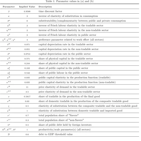
sg;c; sg;i; sw; sl; c; k; n. We assign values to the parameters of the model in three di¤erent ways: (a) based

on parameters widely used in related DSGE models, (b) parameters set to match …rst moments of the Irish

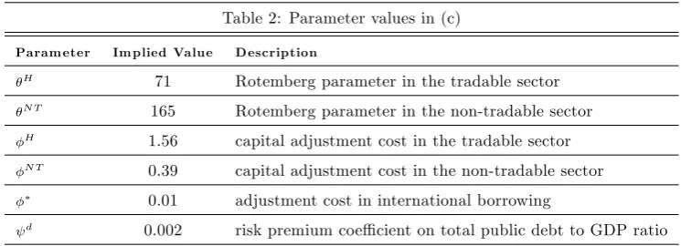
data and (c) parameters set to match second moments of the Irish data. The time unit is a year.

4.1

Parameters widely used in related DSGE models

We employ conventional parameter values used in the DSGE literature for the …fteen structural parameters

that belong to this category. In particular the inverse of the elasticity of intertemoral substitution, ; is set

equal to 2, the preference parameter which measures the degree of substitutability/complementarity between

private and public goods, #g; is set equal to 0 in the benchmark calibration (in section 7.4 we relax this

assumption); the inverse of the Frisch elasticity of labour supply for tradable, H_{; non-tradable,} N T_{; and}

2 6_{The exchange depreciation rate is exogenous since Ireland participates in a currency union, for simplicity we assume}

public, g;hours worked is set equal to 2, the intratemporal elasticity of substitution between the composite

tradable good and the non-tradable good, ; is set equal to 0.5, the intratemporal elasticity of substitution

between the domestic absorption of the home produced tradable good and the imported good, H;is set equal

to 1. H ₌ N T ₌ g_{are set equal to 4 so as the weighted average of hours worked to be equal to 0.4, 0.38 and}

0.31 in the tradable, non-tradable and public sector respectively. The elasticities of substitution among the

di¤erent intermediate good varieties in the tradable,"H_{;and non-tradable sector, "}N T _{, yield price markups}

equal to 1.1 and 1.4 respectively which are consistent with the fact that the tradable sector is more competitive

than the non-tradable sector in Eurozone countries (see also Papageorgiou and Vourvachaki (2017) and Sajedi

(2018)). Finally the scale parameters,AH; AN T; Ag are normalized to 1.

4.2

Parameters set to match …rst moments of the Irish data

The …fteen structural parameters in this category are ; ; H_{; a}H_{; a}N T_; H_; N T_; H

; N T; g; g; Q ;

d; r_; nr_{: The value of the time preference rate is implied by equation (12), = 1=Q; where in steady}

stateQ =R =Q = 1:043 (in‡ation is normalized to 1): Q is the sum of the world interest rate and the

invariant component of Ireland’s interest rate premium. In turn, R = Q = 1:043 follows from setting the

gross interest rate equal to the average value of the real interest rate plus the invariant component of the Irish

sovereign premium.27 _{Structural parameters and} H _{capture the degree of openness of the Irish economy.}

In particular, 1 , governs the share of the non-tradable input in the production of the …nal good, thus

this implicitly determines the size of the non-tradable sector vis-a-vis the tradable sector in gross value added

terms. To calibrate, ; we target the ratio of the gross value added produced in the non-tradable sector to

the sum of value added produced in the tradable and non-tradable sectors. This share is equal to 41% in the

Irish economy. To do this, we add the following restriction when we solve for the steady state solution of the

model:

PN T_yN T

PH_yH_+PN T_yN T = 0:41 (63)

2 7_{We de…ne Ireland’s sovereign risk premium as the di¤erence between Ireland’s and Germany’s nominal interest rates on 10}

This implies that the associated tradable share, _PH_yHP₊H_PyN TH _yN T;is equal to 59%. The parameter, H;governs

the share of domestic absorption of home produced tradable good vis-a-vis the imported good and implicitly

determines the share of the home produced tradable good that it is exported abroad. To calibrate this

parameter we target the value added export share in GDP which is equal to 52%28. Thus we impose:

PH_x

P ygdp = 0:52 (64)

The parameter,1 aH_{;is calibrated to match the average value of the labour share in the tradable sector}

over 2001-2014 which is equal to 0.39:

P wH_lH

PH_yN T = 0:39 (65)

which implies thataH equal to 0.571 is consistent with the capital intensity of the tradable sector. Similarly,

the labour share in the non-tradable sector, 1 aN T;is calibrated to match the average value of the labour

share in the non-tradable sector we observe in the Irish data, so we impose:

P wN T_lN T

PN T_yN T = 0:54

which in turn yieldsaN T _{equal to 0.244 indicating the labour intensity of the non-tradable sector}29_{. The shares}

of public capital in the production functions of both sectors, H _and N T_{;are set equal to the average public}

investment to GDP ratio found in the data as in Baxter and King (1993), i.e. are set equal to 0.035. The

depreciation rates, H; N T; g;are calibrated by constructing time series for the private and public capital

stock employing the methodology in Coenen, Karadi, Schmidt, and Warne (2018) and Gogos, Mylonidis,

Papageorgiou, and Vassilatos (2014). The associated values are H = 0:071; N T = 0:051 and g = 0:0741

(see Appendix I for details). The threshold value, _D; above which the sovereign risk premia emerge, is set

equal to 60%. That is the average value of the Irish public debt to GDP ratio between 2001 and 2014 and also

coincides with the limit imposed by the Maastricht Criteria for all EU countries. Finally, we set the fraction

2 8_{In the model exports and imports are value added while national accounts provide data on gross exports and imports which}

include intermediate goods. For that reason, we employ data from OECD-TiVA database which provide data on exports in value added (time series Domestic value added embodied in foreign …nal demand "FFD_DVA"). Irish data are only available for 2001-2011. We calibrate the model to match exports expressed in value added terms and the trade balance as share of GDP and thus we obtain residually a value for imports.

of "Savers" to total population, r;equal to 0.7, which is consistent with data reported in the Irish module of

the Household Finance and Consumption Survey30 (2013) and in line with values reported in previous studies,

e.g. Forni et al. (2009), Coenen, Straub, and Trabandt (2013), Papageorgiou (2014).

Table 1: Parameter values in (a) and (b)

Param eter Im plied Value D escription

0:9588 time discount factor

2 inverse of elasticity of substitution in consumption

#g _{0 substitutability/complementarity between public and private consumption} H

2 inverse of Frisch labour elasticity in the tradable sector

N T _{2 inverse of Frisch labour elasticity in the non-tradable sector}

P

2 inverse of Frisch labour elasticity in public sector

H_; N T_; g _{4 preference parameter related to work e¤ort (all sectors)} H

0:071 capital depreciation rate in the tradable sector

N T _{0:051 capital depreciation rate in the non-tradable sector} g

0:0741 capital depreciation rate in the public sector

aH _{0:571 share of physical capital in the tradable sector}

aN T 0:244 share of physical capital in the non-tradable sector

ag₁ 0:183 share of public capital in the public sector

ag2 0:542 share of public labour in the public sector

H _{0:035 public capital elasticity in the production function (tradable)} N T

0:035 public capital elasticity in the production function (non-tradable)

"H _{11 price elasticity of demand in the tradable sector}

"N T 3:5 price elasticity of demand in the non-tradable sector 0:5817 share of tradable in the production of the …nal good

H

0:03 share of domestic tradable in the production of the composite tradable good 0:5 elasticity of substitution between the composite tradable and the non-tradable good

H

1 elasticity of substitution between domestic tradable and imported good

r _{0:7 total population share of "Savers"} nr

0:3 total population share of "non-Savers"

g _{0:5 share of public debt held by foreign investors}

AH; AN T; Ag 1 productivity/scale parameter(s) (all sectors)

D 0:6 debt to GDP threshold value

3 0_{In Household Finance and Consumption Survey (2013) is reported that 88.6% of Irish households own a savings account}