Bayesian linear size and shape regression with applications to face data

Bayesian linear size-and-shape regression with

applications to face data

Ian L. Dryden, Kwang-Rae Kim and Huiling Le,

School of Mathematical Sciences, University of Nottingham, UK.

Abstract

Regression models for size-and-shape analysis are developed, where the model is specified in the Euclidean space of the landmark coordinates. Statistical models in this space (which is known as the top space or ambient space) are often easier for practitioners to understand than alternative models in the quotient space of size-and-shapes. We consider a Bayesian linear size-and-shape regression model in which the response variable is given by labelled configuration matrix, and the covariates represent quantities such as gender and age. It is important to parameterize the model so that it is identifiable, and we use the LQ decomposition in the intercept term in the model for this purpose. Gamma priors for the inverse variance of the error term, matrix Fisher priors for the random rotation matrix, and flat priors for the regression coefficients are used. Markov chain Monte Carlo algorithms are used for sampling from the posterior distribution, in particular by using combinations of Metropolis-Hastings updates and a Gibbs sampler. The proposed Bayesian methodology is illustrated with an application to forensic facial data in three dimensions, where we investigate the main changes in growth by describing relative movements of landmarks for each gender over time.

1

Introduction

Bayesian linear regression analysis has been extensively studied for various types of response vari-ables and covariates, where prior distributions are specified for the parameters in the classical re-gression model and statistical inference is carried out using the joint posterior distribution of the parameters (Gelman et al.,2013).

We wish to explore regression models for landmark data, where the location and orientation of the objects can be ignored. Such objects can be represented as points in the size-and-shape space (Dryden and Mardia,2016, Chapter 5), which is defined as the space of landmark co-ordinates after rotation and translation information has been removed (Kendall, 1989). The shape space on the other hand (Dryden and Mardia,2016, Chapter 4) is the space of landmark co-ordinates after rotation, translation

and scaleinformation has been removed (Kendall,1986). Throughout this paper we will concentrate on size-and-shape rather than shape.

An alternative approach is to specify a statistical model in the Euclidean space of the landmark co-ordinates and then integrate out the unwanted location and rotation information by considering the marginal distribution of size-and-shape. In this case, the space in which the statistical model is specified is called the top space in differential geometry, and also known as the ambient space by some authors (Cheng et al.,2016). A top space modelling approach has the advantage that the model is often easier to understand than a quotient space model, and relatively standard inference methods can be used. We shall develop a Bayesian linear model in the space of the Euclidean landmark co-ordinates, and carry out statistical inference using Markov chain Monte Carlo (MCMC) algorithms. Care needs to be taken with identifiability of parameters in the model, and this issue often arises in high-dimensional object data (Dryden,2014).

We consider a Bayesian regression model with response given by the size-and-shape of landmarks with real-valued covariates. A wide variety of regression problems on non-Euclidean spaces have been considered in previous work, and a summary of some approaches is given byDryden and Mardia (2016, Section 13.4). Some approaches include directional data regression (Mardia,1975;Mardia and Jupp,2000;Presnell et al.,1998), tangent space regression models (Kent et al.,2001;Bowman,2008; Faraway,2004), growth curve models (Goodall and Lange,1989), geodesic regression (Le and Kume, 2000;Hotz et al.,2010), principal geodesic analysis (Fletcher et al., 2004;Fletcher, 2013), geodesic PCA (Huckemann et al., 2010; Kenobi et al., 2010), principal nested spheres (Jung et al., 2012), intrinsic regression (Davis et al., 2007; Shi et al., 2009; Hinkle et al., 2014; Cornea et al., 2017), sphere-on-sphere regression (Rosenthal et al., 2014;Rosenthal et al.,2017; Di Marzio et al., 2018), unrolling and unwrapping (Jupp and Kent,1987;Kume et al.,2007), manifold splines (Su et al.,2012) and many applications (e.g.Machado and Leite,2006;Zhu et al.,2009;Samir et al.,2012;Yuan et al., 2012;Piras et al.,2014).

The remainder of this paper is organized as follows. In Section 2 we describe the Bayesian linear size-and-shape regression model, including the prior and posterior distributions. In Section

3, methods for Bayesian inference for the coefficients and model selection are presented. Finally an application to forensic facial data is given in Section4.

2

Bayesian linear size-and-shape regression model

2.1

Linear model

Consider a random sample of n configurations of k labelled landmarks in m dimensions, where each configuration is represented by a k ×m matrix Yi ∈ Rk×m, k > m, i = 1, . . . , n. We are

interested only in the size-and-shapes of Yi after removing translation and rotation, but preserving

scale information (Dryden and Mardia,2016, Chapter 5). In addition we have real valued covariates

xij, j = 1, . . . , p, corresponding to each configuration and without loss of generality we assume that

each covariate is centred, i.e. P

ixij = 0. Categorical variables withg levels can be represented by

g−1binary indicator variables in the standard way. We writexi = (1, x1j, . . . , xpj)> as a(p+

1)-dimensional column vector containing thepcovariates and1for the intercept. We aim to predict the size-and-shape ofYiusing the covariates, and explore the relationship betweenYiandxi,i= 1, . . . , n.

Suppose thatYiare modelled with a probability distribution with conditional mean functionµ(xi)

given covariatesxi and subject to an arbitrary unknown rotationΛi ∈ SO(m), whereSO(m)is the

group of special orthogonal matrices that satisfyΛiΛ>i = Λ

>

is them×midentity matrix. So we have the conditional mean

E[Yi|xi] =µ(xi)Λi, i= 1, . . . , n.

Including a noise term we have the model

Yi =µ(xi)Λi+εi,

whereεi are assumed to be i.i.d. random matrix normal variables of dimension k×m (Gupta and

Nagar, 1999, Chapter 2). In this paper we consider the conditional mean functionµ(xi)to be linear

so that the following linear regression model is of interest,

Yi = α0+

p

X

j=1

αjxij

!

Λi+εi, (1)

whereα0, αj ∈ Rk×m, j = 1, . . . , p, arek×mregression parameter matrices, the errors are matrix

normal

εi

i.i.d.

∼ M Nk×m 0, σ2Im, Ik

,

and so

vec(εi) i.i.d.

∼ Nkm vec(0), σ2Im⊗Ik

,

where vec(A)denotes the vectorization of the matrix A (i.e. stacking columns) and⊗ denotes the Kronecker product. The model (1) is not identifiable since the rotation effect from Λi dictates the

coefficients {α0, αj}. We can make the model identifiable using an LQ decomposition of α0. In particular we writeα0 = β0Q0, whereQ0 ∈ SO(m)andβ0 is lower triangular (i.e. has zero entries above the leading diagonal). Therefore the model (1) can be rewritten as

Yi = µ(xi)Γi+εi,

= β0+

p

X

j=1

βjxij

!

Γi+εi

= XiβΓi +εi, (2)

whereXi =x>i ⊗Ik ∈Rk×k(p+1) is ak×k(p+ 1)matrix,β =

β₀> β₁> · · · β_p>> ∈_Rk(p+1)×m

is ak(p+ 1)×mmatrix of regression parameters andΓi ∈ SO(m). In the following we describe a

Bayesian approach to estimateµ(xi)given deterministic covariatesxi.

2.2

Likelihood

It follows from the matrix normality ofεi thatYi ∼M Nk×m XiβΓi, σ2Im, Ik

,therefore the proba-bility density function ofYi is given by

f(Yi |β,Γi, σ2) =

1

(2πσ2₎km/2 exp

− 1

2σ2 tr

(Yi−XiβΓi)>(Yi−XiβΓi)

and the likelihood is given by

f(Y1, . . . , Yn,|β,Γ1, . . . ,Γn, σ2) =

1

(2πσ2₎nkm/2 exp − 1 2σ2

n

X

i=1

tr(Yi−XiβΓi)>(Yi−XiβΓi)

!

2.3

Prior and posterior

We shall concentrate on the m = 3 dimensional case and it is then helpful to adopt a particular parameterization of the rotation matrices. We can represent the three dimensional rotation matrix using theZXZ-convention where

Γ(θ1, θ2, θ3) =  

cosθ3 sinθ3 0

−sinθ3 cosθ3 0

0 0 1

 

 

1 0 0

0 cosθ2 sinθ2 0 −sinθ2 cosθ2

 

 

cosθ1 sinθ1 0

−sinθ1 cosθ1 0

0 0 1

 ,

0≤ θ1, θ3 < 2π and0≤ θ2 < π (Landau and Lifschitz, 1976). If we assume thatθ1, θ3 ∼ U[0,2π)

andθ2 ∼U[0, π), then using these co-ordinates the density of the uniform distribution onSO(m)is

g(θ1, θ2, θ3) =

1 2π

1 2sinθ2

1

2π ∝sinθ2. (3)

We consider the following priors for parameters(κ,Γi, β). Letκ= 1/σ2. Assume thatκfollows

a Gamma distribution with shape parameter a and scale parameterb. We consider the prior for the rotation matrix to be the matrix Fisher distribution (Mardia and Jupp, 2000, p.89) and F0 is a3×3 parameter matrix of that so thatp(Γi;F0) ∝ exp{tr(F0>Γi)}sinθi2 andsinθi2 is due to the uniform measure. The regression parametersβare taken to be uniform and all the parameters are independent, i.e.

κ∼Gamma(a, b) ;

Γi ∼matrix Fisher(F0), i= 1, . . . , n ;

p(β |Γ1, . . . ,Γn, κ)∝1,

independently. Then the joint posterior density for(β,Γ1, . . . ,Γn, κ)is given by

p(β,Γ1, . . . ,Γn, κ|Y1, . . . , Yn)

∝ exp

n

X

i=1

tr(F₀>Γi)

! " n

Y

i=1

sinθi2

#

κa+3nk/2−1exp−κ

b

exp −1

2κ

n

X

i=1

tr(Yi−XiβΓi)>(Yi−XiβΓi)

!

.

The conditional posterior for(κ|Γ1, . . . ,Γn, β, Y1, . . . , Yn)is

κ|Γ1, . . . ,Γn, β, Y1, . . . , Yn ∼Gam

   

a+ 3nk

2 ,

1

1

b +

1 2

Pn

i=1tr

Yi−XiβΓi

>

Yi−XiβΓi

   

.

The conditional posterior for(β |Γ1, . . . ,Γn, κ, Y1, . . . , Yn)is

vec(β>)(−0) |Γ1, . . . ,Γn, κ, Y1, . . . , Yn ∼N3k(p+1)−3 vec(ξ>)(−0),(Ω⊗Σ)(−0)

,

where

Σ = 1

κI3,

Ω =

n

X

i=1

X_i>Xi

!−1

,

ξ =

n

X

i=1

X_i>Xi

!−1 _n X

i=1

and

vec(β>) =     

vec(β₀>) vec(β₁>)

.. . vec(β_p>)

    

, vec(ξ>) =

    

vec(ξ>₀) vec(ξ>₁)

.. . vec(ξ>_p)

    

with size     

3k×1 3k×1

.. . 3k×1

    

,

Ω⊗Σis a3k(p+1)×3k(p+1)covariance matrix, and(−0)stands for removing2th,3th,6th elements of vec(β>)and vec(ξ>), and also removing those three rows and columns ofΩ⊗Σ. Hence for each vec(β₀>)(−0)_,vec(β>

1), . . . ,vec(β

>

p)of length3k−3,3k, . . . ,3k, we can use the following conditional

distribution of partitioned multivariate normal distribution

vec(β₀>)(−0) |Γ1, . . . ,Γn, κ, Y1, . . . , Yn,vec(β1>), . . . ,vec(β

>

p ),

vec(β_j>)|Γ1, . . . ,Γn, κ, Y1, . . . , Yn,vec(β0>)(

−0)_,vec(β>

−j), j = 1, . . . , p.

The conditional posterior for(Γ1, . . . ,Γn |κ, β, Y1, . . . , Yn)is proportional to

exp

n

X

i=1 tr

(F0+κβ>Xi>Yi)>Γi

! " _n

Y

i=1 sinθi2

#

.

Hence for a specific ith observation, using independence the conditional posterior for Γi is

propor-tional to

Γi |Γ−i, κ, β, Y1, . . . , Yn∝exp tr

F_i>Γi

sinθi2,

where

Fi =F0+κβ>Xi>Yi, i= 1, . . . , n.

Let us drop the observation indexifor a moment then

tr(F>Γ) = C1cosθ1+S1sinθ1+R1 = C2cosθ2+S2sinθ2+R2 = C3cosθ3+S3sinθ3+R3,

where

C1 = F11cosθ3−F21sinθ3+F12sinθ3cosθ2+F22cosθ3cosθ2−F32sinθ2,

S1 = −F11sinθ3cosθ2−F21cosθ3cosθ2+F31sinθ2+F12cosθ3−F22sinθ3,

C2 = −F11sinθ3sinθ1−F21cosθ3sinθ1+F12sinθ3cosθ1+F22cosθ3cosθ1+F33,

S2 = F31sinθ1+F13sinθ3+F23cosθ3−F32cosθ1,

C3 = F11cosθ1−F21cosθ2sinθ1+F12sinθ1+F22cosθ2cosθ1+F23sinθ2,

S3 = −F11cosθ2sinθ1−F21cosθ1+F12cosθ2cosθ1−F22sinθ1+F13sinθ2,

andR1, R2, R3 are remainder terms independent of each Euler angle. Hence forith observation, the conditional distributions forθi1andθi3 are von Mises distributions (Green and Mardia,2006). Since

θi2 |θi1, θi3,Γ−i, κ, β, Y1, . . . , Yn∝exp (Ci2cosθi2+Si2sinθi2) sinθi2,

Remark(Helmertized size-and-shape. LetYH

i = HYi be Helmertized size-and-shapes, whereH

is the Helmert sub-matrix (Dryden and Mardia,2016, p.49-50). It is often useful to work withYH

i as

this takes care of the location invariance for size-and-shapes, and reduces the number of parameters appropriately.

Condition(Identifiability). Consider the Helmertized model

Y_iH = β0+

p

X

j=1

βjxij

!

Γi+εi,

whereβj, j = 0,1, . . . , p,are(k−1)×3matrices. LetGbe the number of distinct sets of covariate

tuples in(x1, . . . ,xn), then fork ≥4

p1 =G{3(k−1)−3}=G(3k−6)

is the number of regression parameters that can be identifiable. Let

p2 ={3(k−1)−3}+p{3(k−1)}= (3k−6) +p(3k−3) = 3k(p+ 1)−6−3p

be the number of parameters in regression model. Then all p2 parameters in regression model are identifiable ifp1 ≥p2.

This identifiability condition indicates that the stability of estimation depends on how many dis-tinct tuples of covariates are used. Ifp1 < p2then MCMC draws of parameters can be away from the true values due to non-identifiability, or we may need a long number iterations ifp1 =p2.

3

Inference and model selection

3.1

Inference for the coefficients

After the posterior sample {β_j(t), j = 0, . . . , p, t = 1, . . . , T} is obtained from T iterations of the MCMC algorithm after burn-in, we can make an inference for β. Marginal100(1−α)% credible intervals forβj, j = 0, . . . , p, are given by

βj,α/2, βj,1−α/2

,

whereβj,P denotes the quantile at probabilityP based on order statistics from the sample after

burn-in. Sinceβ_j(t)is a matrix we define the matrix quantile as an element-wise quantile. An alternative approach based on marginal Gaussian distributions forβj is

h b

βj−zα/2·sd\(βj), βb_j +z_α/2·sd\(β_j)

i

,

where

b

βj =

1

T

T

X

t=1

β_j(t),

\

sd(βj) =

v u u t

1

T −1

T

X

t=1

β_j(t)−βb_j

◦ β_j(t)−βb_j

,

and◦is the Hadamard product defined by(X◦Y)i,j = (X)i,j·(Y)i,j for two matricesX andY of

3.2

Model selection

We now present measures for model selection. For convenience writeΘ = (β,Γ1, . . . ,Γn, σ2) and

letL(Y |Θ)be the likelihood function. Define the deviance asD(Θ) =−2 log L(Y |Θ), then the deviance information criterion (DIC) is defined by penalizing the deviance by the effective number of parameters,pD (Spiegelhalter et al.,2002)(Gelman et al.,2013, p.172), i.e.

DIC = D+pD

= D(Θ) + 2pD,

whereD=_E[D(Θ)]is the posterior expected deviance andΘis the posterior mean ofΘ. In practice the posterior expectations are obtained from the arithmetic means of the relevant terms from a MCMC algorithm after burn-in. The effective number of parameters can be estimated by eitherp(1)_D = D− D(Θ)(Spiegelhalter et al.,2002) orp(2)_D = 1₂var D(Θ)(Gelman et al.,2013, p.173).

The Watanabe-Akaike information criterion or widely available information criterion (WAIC) (Watanabe,2010) (Gelman et al.,2013, p.173) is a fully Bayesian criterion based on the log pointwise posterior predictive density adjusted by the effective number of parameters,pWAIC, to avoid overfitting and is defined by

WAIC=−2 ( _n

X

i=1

log _Ef Yi |β,Γi, σ2

+pWAIC )

,

where again we have two possible estimates of the effective number of parameters:

pWAIC1 = 2

n

X

i=1

log _E

f Yi |β,Γi, σ2

−_E

logf Yi |β,Γi, σ2

,

pWAIC2 =

n

X

i=1 var

logf Yi |β,Γi, σ2

.

The Akaike information criterion (AIC) (Akaike,1973) and the Bayesian information criterion (BIC) (Schwarz,1978) are defined by

AIC = −2 log L(Y |Θmle)

+ 2K,

BIC = −2 log L(Y |Θmle)

+Klogn,

whereΘmleis the sample point where the log-likelihood function is maximised after burn-in andK is

the number of parameters, so thatK = 3(k−1)p−3+n+1. It is well known that AIC is minimax-rate optimal in estimating the regression function (Barron et al.,1999;Yang,2005), and BIC is consistent in model selection (Shao, 1997;Yang, 2005). Note that the model which has smaller DIC, WAIC, AIC or BIC provides a better model.

4

Application to forensic facial data

4.1

Data description

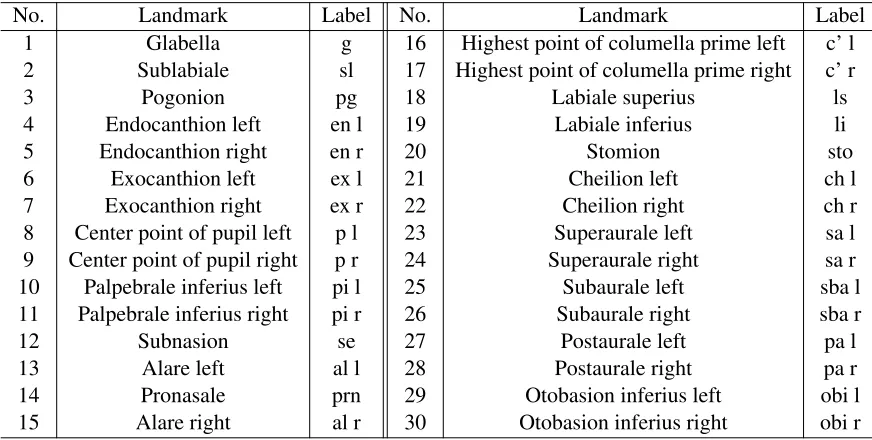
to be important covariates when describing the size and shape of the face landmark configurations, and so we develop some Bayesian regression models to explore the relationship. A set of 3D facial images was captured by a Geometrix FaceVision FV802 Series Biometric camera and then 30 an-thropometric landmarks in 3D were selected by trained observers. The volunteers in the study were primarily scanned at the Magma Science Adventure Centre, Rotherham, UK. Evison and Bruegge (2010, Chapter 3) give full details of the project and provide discussion about the selection of the 30 landmarks. Many of the face landmark sets were recorded twice, either with different observers or the same observer. In total we have3248 face landmark configurations from 1964volunteers, in particular956faces from 627females and2292faces from1337males. The landmark positions and descriptions are described in Table1 followingEvison and Bruegge (2010). Our main interest here involves investigating the relation between age and the size and shape of the faces for each gender.

Table 1: Landmark information (Evison and Bruegge,2010)

No. Landmark Label No. Landmark Label

1 Glabella g 16 Highest point of columella prime left c’ l 2 Sublabiale sl 17 Highest point of columella prime right c’ r

3 Pogonion pg 18 Labiale superius ls

4 Endocanthion left en l 19 Labiale inferius li

5 Endocanthion right en r 20 Stomion sto

6 Exocanthion left ex l 21 Cheilion left ch l

7 Exocanthion right ex r 22 Cheilion right ch r

8 Center point of pupil left p l 23 Superaurale left sa l 9 Center point of pupil right p r 24 Superaurale right sa r 10 Palpebrale inferius left pi l 25 Subaurale left sba l 11 Palpebrale inferius right pi r 26 Subaurale right sba r

12 Subnasion se 27 Postaurale left pa l

13 Alare left al l 28 Postaurale right pa r

14 Pronasale prn 29 Otobasion inferius left obi l

15 Alare right al r 30 Otobasion inferius right obi r

As would be expected on average male faces are larger and wider than female faces as shown in Figure1 (a), where the main growth direction corresponds to the first shape principal component’s direction indicated by black lines in Figure1(b),(c). SeeDryden and Mardia(2016, Section 7.7-7.8) for a summary of principal components analysis in shape and size-and-shape analysis, which has been implemented inRfunctionsprocGPA()andshapepca()in the packageshapes(Dryden, 2017). In order to measure the size of the face landmark configuration, we use the centroid size of a configurationXgiven by

S(X) =kHXk,

whereH is the Helmert submatrix (Dryden and Mardia, 2016, p.49) andkXk = ptrace(X>_X).

(a) Front view of size-and-shape configu-rations.

(b) Female (c) Male

Figure 1: (a) Front view of size-and-shape configurations. (b), (c) Mean (red) and 3 PCs direction in +3·sd (black: PC1, red: PC2, green: PC3).

−50 −25 0 25 50

360 380 400

Size

Siz

e−and−shape PC1 (18%)

(a) Female

−50 −25 0 25 50

380 400 420 440

Size

Siz

e−and−shape PC1 (19%)

(b) Male

4.2

Models and implementation

Recall from Section2.1that the intercept matrixβ0is lower triangular using an LQ decomposition for model identifiability, and the procedure is more stable if the landmarks in the first three positions are well separated. Hence in this application we re-ordered the landmarks as(1,3,30,2,4,5, ...,28,29). Note that the inference is invariant to a ordering of the landmarks, and so in theory such a re-ordering should make no difference in our modelling. However, in computational implementation it is best to avoid having the the first three landmarks too close together as otherwise some numerical in-stabilities can appear due to the standardisation via the LQ decomposition. The proposed re-ordering leads to stable results, which would in practice be equivalent to any other reordering with well sepa-rated landmarks in the first three positions.

For each gender we use the following three Helmertized models, where the Helmertizing takes care of the location invariance:

M1: Y_iH = {β0+β1agei}Γi+εi,

M2: Y_iH =

β0+β1agei+β2age2i Γi+εi

M3: Y_iH =

β0+β1agei+β2age3i Γi+εi,

whereYH

i = HYi, i = 1, . . . , n. We consider a weakly informative conjugate prior κ so that a =

0.001andb = 1000(Spiegelhalter et al.,2003), and the hyperparameterF0in the prior distribution for the rotation parameters is taken as a3×3matrix of zeroes. For the MCMC algorithm we set the initial value ofβto0,Γi, i= 1, . . . , n,to3×3identity matrices, andκto a random draw from Gamma(a, b).

The Gibbs samplers of Section2.3 are used for updating (κ, β, θ1, θ3)and in order to update θ2 via the Metropolis-Hastings algorithm we use a normal distribution with standard deviationσθ2 = 0.3as the proposal distribution. To obtain a centred predicted face configuration we pre-multiply each fitted valueYbibyC, for example for M2:

CYbi =

n

H>βb0+H>βb1agei+H>βb2age2i

o b Γi,

where C = Ik− 1_k1k1>k, Ik is the k ×k identity matrix, 1k is the column vector of k ones, βb_j = 1

T

PT

t=1β

(t)

j , bΓ_i = _T1 PT

t=1Γ

(t)

i are the arithmetic means of the MCMC sample ofT iterations forβj

andΓi after burn-in, and in our faces application we havek = 30landmarks.

4.3

Results

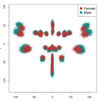
We run the MCMC chain for 200,000 iterations with 100,000 iterations of burn-in. The Metropolis-Hastings acceptance rate forθ2 is around 3.72% for female and 3.83% for male data. The posterior variance for females is smaller than that for males as the posterior mean estimates forκ are larger than those for males in Table2.

For the three models considered, model M2 is generally the best model for both female and male groups since M2 outperforms the others in terms of the model selection statistics DIC, WAIC and AIC in Table3(except that M1 has the smallest BIC for females). We now investigate the structure of the models of the fitted size-and-shapes of the face landmarks versus age and gender.

Table 2: Estimates forκand acceptance rate forθ2.

Model Posterior meanκ 95% cred.int. κ Acceptance rateθ2

Female

M1 0.1124 (0.1115, 0.1133) 3.73%

M2 0.1127 (0.1118, 0.1136) 3.72%

M3 0.1127 (0.1117, 0.1136) 3.72%

Male

M1 0.0911 (0.0906, 0.0916) 3.85%

M2 0.0925 (0.0920, 0.0930) 3.83%

M3 0.0924 (0.0919, 0.0929) 3.83%

Table 3: Model selection statistics. Note that the best model for each line is indicated in bold.

Statistics Female Male

M1 M2 M3 M1 M2 M3

# of parameters 1128 1215 1215 2464 2551 2551

Maximum log-likelihood -208753 -208635 -208649 -521561 -520026 -520187 DIC 420986 420837 420881 1050933 1047960 1048246 WAIC1 415056 414899 414944 1036202 1033334 1033605 WAIC2 416164 416020 416067 1038860 1035994 1036264 AIC 419763 419699 419727 1048050 1045155 1045475 BIC 425248 425607 425636 1062187 1059790 1060111

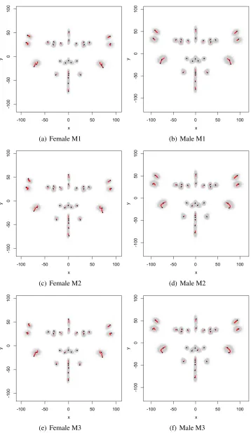
face. The fitted configurations can be arbitrarily rotated, and in order to compare the fitted configura-tions over age with the size-and-shapes of the Procrustes registered data, we apply ordinary Procrustes analysis to translate and rotate the fitted faces from the model (in red) onto the Procrustes mean size-and-shape of the data. The fitted faces are indicated by a red curved line from the fitted face at age 15 through to the fitted face at age 80 (which is identified with a black dot).

The fitted models for the females and males show important differences in Figure3. In particular it is noticeable that the amount and direction of facial growth as age increases differ between females and males. For model M1, the males’ fitted face linearly grows as age increases but the change is different for females as age increases. In some areas such as the eyes and ears, the face grows quicker later for females. The growth direction of the ears of females is relatively wider than that for males. The credible intervals for age for eight landmarks on the ears (landmarks 23 – 30), indicated by red line thickness, are relatively longer than the others for both the females and males. On the other hand, the credible intervals for the eight landmarks on the eyes (landmarks 4 – 11) are relatively shorter. For models M2 and M3, it is notable that the growth direction of the four landmarks on the bottom of the ears (landmarks 29, 30, 25 and 26) is different for females and males, where the females’ ears grow wider than the males’. The results of models M2 and M3 are more similar to each other than M1 for both females and males. This observation can be inferred from Table3showing smaller differences in the model selection criteria for M2 versus M3 compared to M1 versus M2.

(a) Female M1 (b) Male M1

(c) Female M2 (d) Male M2

(e) Female M3 (f) Male M3

(a) Female: ear, top left. (b) Female: ear, top right.

(c) Male: ear, top left. (d) Male: ear, top right.

(e) Female: ear, bottom left.

(f) Female: ear, bottom right.

(g) Male: ear, bottom left. (h) Male: ear, bottom right.

(i) Female: lips. (j) Male: lips.

behaviour is different before and after the turning point. The age at the turning point of the predicted curves can be different depending on the landmark position. We mark blue points to indicate age 37 for female and age 52 for male, and a black dot for age 80. Note that the predicted red points were obtained at equal age intervals. The speed of facial growth varies over age, for example for the top of the ears of females, (a) and (b), the upper parts of the top ears grow slowly for young women but those parts grow rapidly for older women. For the lower parts of the top of the ears, the speed of growth starts slowly and then becomes faster after age 37. For men in (c) and (d), a similar pattern to the lower parts of the top of the ears appears with the turning age 52. For the bottom of the ears and lips, (e) – (j) females and males show opposite results in growing speed, where females grow rapidly as age increases, however males grow slowly as age increases.

0.6

0.8

1.0

1.2

1.4

1.6

1.8

Landmark No.

Length of credib

le inter

v

al (mean)

1 3 5 7 9 11 13 15 17 19 21 23 25 27 29

(a) Female: mean configuration.

0.4

0.6

0.8

1.0

Landmark No.

Length of credib

le inter

v

al (mean)

1 3 5 7 9 11 13 15 17 19 21 23 25 27 29

(b) Male: mean configuration.

0.4

0.6

0.8

1.0

1.2

1.4

1.6

Landmark No.

Length of credib

le inter

v

al (age)

1 3 5 7 9 11 13 15 17 19 21 23 25 27 29

(c) Female:age.

0.3

0.4

0.5

0.6

0.7

0.8

Landmark No.

Length of credib

le inter

v

al (age)

1 3 5 7 9 11 13 15 17 19 21 23 25 27 29

(d) Male:age.

0.004

0.006

0.008

0.010

0.012

Landmark No.

Length of credib

le inter

v

al (age^2)

1 3 5 7 9 11 13 15 17 19 21 23 25 27 29

(e) Female:age2.

0.003

0.005

0.007

Landmark No.

Length of credib

le inter

v

al (age^2)

1 3 5 7 9 11 13 15 17 19 21 23 25 27 29

(f) Male:age2.

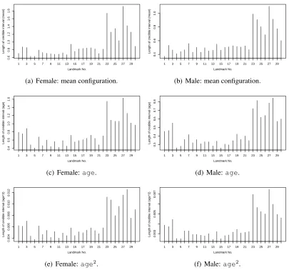
Figure 5: Length of credible interval (M2).

From Figure5(a) and (b) the outer parts of the face have more posterior variability which is shown in the length of the credible intervals for both ears (landmarks 23 to 30). In contrast near the eyes (landmarks 4 – 11), the lengths of credibility intervals are short. When faces grow as age increases for both females and males, the variability near both ears is larger as shown in (c), (d), (e) and (f).

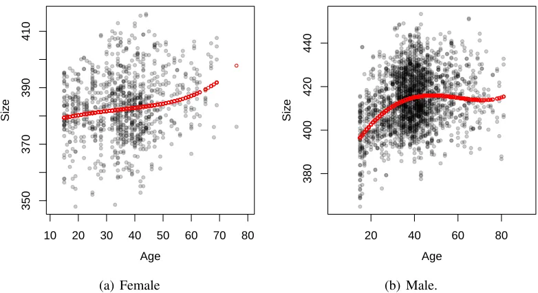
10 20 30 40 50 60 70 80 350 370 390 410 Age Siz e ● ● ● ● ●●●● ●● ● ● ● ● ● ●● ● ● ● ●●● ● ● ●● ● ● ● ● ● ● ● ● ●● ● ● ● ● ● ● ● ● ●● ● ●●●●●●● ● ● ●●●● ● ● ● ●● ● ● ● ● ● ● ● ●● ● ●●● ● ● ● ● ● ● ● ● ● ● ● ● ● ●● ● ● ● ● ● ●● ●● ● ● ● ● ● ● ● ● ● ● ● ● ●● ● ●●● ● ● ●● ● ● ● ● ● ● ● ● ● ● ● ● ● ● ● ● ● ●● ● ● ●● ● ● ● ● ● ● ● ●● ● ● ● ● ●●●●●● ● ● ● ● ● ● ● ● ● ● ● ● ● ● ● ●●● ● ●● ● ●● ● ● ● ● ● ● ● ● ● ●● ● ● ●●● ● ● ●● ● ● ● ● ●● ● ● ●●●● ● ● ● ● ● ● ● ● ● ● ●●●●● ● ● ● ● ● ●●●● ● ● ● ● ● ● ●● ●● ● ● ● ● ● ● ● ● ● ● ● ● ● ● ● ● ● ● ●●● ●● ● ● ●● ●● ● ● ●●● ●● ● ● ● ● ● ● ● ● ● ● ● ● ● ● ● ● ●● ● ●●●●●●● ●●●● ● ● ● ● ●●●● ● ● ● ● ● ● ● ●●● ● ● ●● ● ● ● ● ● ● ● ● ● ● ● ● ● ● ●●●●● ● ● ● ● ● ● ● ●● ● ● ● ● ● ● ● ● ● ● ● ●●● ● ● ● ● ● ● ●●● ●● ● ● ● ● ●● ● ● ●● ● ● ● ●● ● ● ●● ● ● ● ●● ● ● ● ● ● ● ● ● ● ● ● ● ● ● ● ● ● ● ● ● ●●●● ● ● ● ● ● ● ● ● ● ● ● ● ● ● ● ● ● ● ● ●●●●● ●● ● ● ● ● ● ●●● ● ● ● ●●● ● ● ● ●● ● ● ● ● ● ●● ● ● ● ● ● ● ● ● ● ●● ● ●● ● ● ● ● ●●● ● ● ● ● ● ● ● ● ● ● ● ●● ● ● ● ● ● ● ● ● ● ● ● ● ● ● ●● ● ● ●● ● ●●● ●●●● ● ● ● ●●●●●●●●●●●● ● ● ● ● ●● ● ● ● ● ●●● ● ●● ● ● ● ● ● ● ●● ● ● ● ● ● ●●●●● ●●●●●● ● ● ● ● ● ● ● ● ● ● ● ● ●● ● ● ● ● ● ● ● ● ● ● ● ● ● ●● ● ● ● ● ● ● ● ● ● ● ● ● ●●● ● ● ● ● ● ● ● ● ● ● ● ●● ● ● ● ● ● ● ● ● ● ● ● ● ● ● ● ●● ● ● ● ●● ● ●● ● ● ● ● ● ● ● ● ● ● ● ● ● ● ● ● ●● ● ● ● ● ● ● ● ● ● ●● ● ● ● ● ●● ● ● ● ● ●● ●●● ● ● ● ● ● ● ● ● ● ● ● ● ● ● ● ● ● ● ● ● ● ● ● ●●●●●●●● ● ● ● ● ● ● ● ● ● ● ● ● ● ● ● ● ● ● ● ● ● ● ● ●● ● ● ● ● ● ● ● ● ● ● ● ● ● ● ● ● ● ● ● ● ● ● ● ● ● ●● ● ● ●● ●● ● ● ●● ●●● ● ● ● ● ● ● ● ● ● ● ● ● ● ● ● ● ● ● ● ●● ● ● ● ● ● ● ● ● ● ● ● ● ● ● ● ● ● ● ● ● ● ● ● ● ● ● ● ● ● ● ● ● ●●● ● ● ● ● ● ● ● ● ● ● ● ● ● ● ● ● ● ● ●●●●●● ● ● ● ● ●● ● ● ● ● ●● ● ●●●● ● ● ●●● ●● ● ●● ● ● ● ● ● ● ● ● ● ● ● ● (a) Female

20 40 60 80

380 400 420 440 Age Siz

e ● ●

● ●●●●● ●● ● ● ● ●● ● ● ● ● ● ● ● ● ● ● ● ● ● ● ●●● ●● ● ● ● ●● ● ● ● ● ●● ● ● ● ●●● ● ● ● ● ● ● ● ● ● ● ● ● ● ● ●● ●● ● ● ● ● ● ● ● ● ● ●●● ●● ● ● ● ● ● ● ●● ● ● ● ● ● ● ●● ● ● ● ● ● ● ● ● ● ● ● ● ● ●●●●● ● ● ● ● ● ● ● ● ● ● ●● ● ● ●● ● ● ●● ● ●● ●●● ●● ●●●●● ● ● ● ● ● ● ● ● ● ●●●●● ● ● ● ● ● ● ● ● ● ● ●● ● ● ● ● ● ● ● ●● ●● ● ● ● ●●●●●●● ●● ●● ● ● ● ● ●●●● ● ● ● ●● ● ● ● ●●●●●●●● ● ● ●● ● ● ● ● ● ● ● ● ● ● ● ● ●● ● ● ● ● ● ● ●●●●● ● ● ● ● ● ● ●● ●● ● ●●● ●● ● ● ●● ● ● ● ● ● ● ● ● ● ● ● ● ● ● ●●● ● ● ●● ● ●●● ● ●● ● ● ● ●●●●● ● ● ●● ● ●● ● ●● ● ● ● ●●●● ●●● ● ● ● ● ● ● ●●● ●● ● ●●● ● ● ● ● ● ● ● ● ● ● ●● ● ● ● ● ● ● ● ● ●●●●● ●●●●●● ● ● ● ● ● ●●● ●● ● ● ● ●●●●●●●●● ● ● ● ● ● ● ● ●●●●● ● ● ● ●● ● ●● ● ● ● ●●●●● ●●●●●●●●●● ●● ●● ●●_●● ● ● ● ● ● ●●●●●●●● ●●●● ● ● ● ● ● ● ● ● ●● ● ● ● ● ● ● ● ● ● ● ● ●● ● ● ● ● ●● ●● ●●●● ● ●●● ● ● ●●●●● ●●●● ● ● ●● ● ● ● ● ● ● ●● ●● ● ●●● ● ● ● ● ● ● ● ● ● ● ● ● ●●●●● ●● ●●● ●● ● ● ● ● ●●●●● ● ● ● ● ● ● ● ● ● ● ● ● ● ● ● ● ● ● ● ● ● ● ●●●●●●●● ● _●● ● ● ● ● ● ● ● ● ● ● ● ● ●● ● ● ●●●● ●● _●● ● ● ● ● ● ● ● ●● ● ● ●● ● ● ●●● ● ● ● ● ● ● ● ● ● ● ● ● ● ● ●● ●● ● ● ● ● ●● ● ● ● ● ● ● ● ●●●●● ● ● ● ●●● ● ● ●● ● ● ● ● ● ● ● ● ● ● ● ● ● ● ● ● ● ●●● ●● ● ● ● ● _● ● ● ● ● ● ● ● ● ● ● ●●● ● ● ● ● ● ● ● ● ● ● ●● ● ● ● ● ● ● ● ● ● ● ● ● ● ● ● ● ●● ● ● ● ● ● ● ● ● ● ● ● ● ● ● ● ● ● ●●●● ● ● ● ●● ● ● ● ● ●● ● ● ●●●●●● ● ● ● ● ●● ● ● ● ● ● ● ● ● ●●●●●●●●●● ●● ●● ●● ● ●● ● ● ● ● ● ● ● ● ● ● ● ● ● ● ● ● ● ● ●● ● ● ● ● ● ● ● ● ● ● ● ● ● ● ● ● ● ● ● ● ● ● ● ● ● ● ● ● ● ● ● ● ● ● ● ● ● ● ● ● ● ● ● ● ● ● ● ● ● ● ● ● ● ● ● ● ●●●●●●●●●●● ●● ● ● ● ● ● ● _● ● ● ● ● ● ● ● ● ● ● ● ● ● ● ● ● ● ● ● ● ● ● ● ● ● ● ● ● ●● ● ● ● ● ● ● ● ● ● ● ● ● ● ●● ●● ● ● ● ● ● ● ● ●●● ● ●●● ● ●● ●●● ● ●●● ● ● ● ● ● ● ● ● ● ● ● ● ● ● ● ● ● ● ● ● ●●● ● ● ● ● ● ● ● ● ● ● ● ● ● ● ● ●●●● ● ● ● ● ● ● ● ● ● ●● ● ● ● ● ● ● ● ● ●●● ●● ● ●● ● ● ● ● ● ● ● ● ● ● ● ● ● ● ● ● ●● ● ● ● ● ● ● ● ● ● ● ●● ● ● ●● ● ● ● ● ● ● ● ● ● ● ● ● ● ● ● ● ● ● ● ● ● ● ● ● ● ● ●●● ● ● ● ●●● ●● ● ● ● ● ●● ● ● ●●● ● ● ●● ● ●● ● ● ● ●● ● ● ●● ● ● ● ● ● ● ● ● ● ● ● ● ● ● ● ● ●●●●● ● ● ● ● ● ● ● ● ● ●●●●●●● ●●●●●●● ● ● ● ● ● ● ●●●●● ●●●● ● ● ●● ● ● ● ● ●●●●● ●● ● ● ● ● ● ● ● ●● ● ● ● ● ● ●● ● ● ● ● ● ● ● ● ● ● ● ● ● _●● ● ● ● ● ● ● ● ● ●● ● ● ● ● ● ●● ● ●●● ● ● ● ● ● ● ● ● ● ● ● ● ● ●● ● ● ● ● ●●●● ● ● ● ● ● ● ● ● ●● ● ● ● ● ● ● ● ● ● ● ● ●● ● ●●● ●● ● ● ● ● ● ●● ● ● ●● ●● ● ● ●●● ●●●● ● ● ●●●● ● ● ● ● ● ● ● ●● ● ● ● ● ● ● ●●●●●●●●● ● ● ● ●● ● ● ● ● ● ● ●● ● ● ● ● ● ● ● ● ● ● ● ● ● ●●● ● ●●● ● ● ● ● ● ● ●● ●●● ● ● ● ● ● ● ● ● ● ● ● ● ● ● ● ● ● ● ● ● ● ● ● ● ●●●●● ● ● ● ● ● ● ● ● ● ● ● ● ● ● ● ● ● ● ● ● ● ● ● ● ● ● ● ●●● ● ● ● ● ●● ● ●●●●●● ●●● ● ● ● ● ● ●●●●●● ● ● ●●●● ●●●●●●●●●●●●●●●● ● ● ●●●●●●●●●●●●●●●●●●●●● ● ● ● ●●● ● ● ● ● ● ● ● ● ● ●● ●● ● ● ● ● ● ● ●● ● ● ● ● ● ● ● ● ● ● ● ● ● ● ●●●●● ● ● ●● ● ● ● ● ● ●●● ● ● ● ● ●●● ● ● _●● ● ● ● ●● ● ●● ●● ● ● ● ● ● ● ● ●● ● ● ● ● ●●●● ●● ● ● ● ● ● ● ● ● ● ● ● ● ● ● ● ● ●●●●● ● ● ● ● ● ● ● ● ● ● ● ● ● ● ● ● ● ● ● ● ● ● ● ● ● ● ● ● ● ● ● ● ● ● ● ● ● ● ● ● ●●● ● ● ● ● _●● ● ●●● ● ● ● ● ● ● ● ● ● ● ● ● ● ● ● ● ● ● ● ● ● ● ● ● ● ● ● ● ●●●●●● ●● ●● ● ● ● ●●● ●●● ● ● ● ● ● ● ● ● ● ●●● ●● ● ● ● ● ● ●● ●● ● ● ● ● ● ● ● ● ● ●●● ● ● ●●● ● ● ● ●● ● ● ● ● ● ● ● ● ● ● ● ● ●● ● ● ● ● ● ●● ● ●● ● ● ● ● ● ●●●● ●● ● ● ● ●● ●● ● ● ● ● ● ● ●●● ● ● ●●● ●● ● ● ● ● ●● ● ● ● ●● ● ● ● ● ● ● ● ● ● ● ●●● ● ● ● ● ● ● ● ● ● ● ● ● ● ● ● ● ● ● ● ● ● ●●● ● ● ●● ● ● ● ●●●●● ● ● ● ●● ●●● ●● ● ● ●● ● ● ● ●●● ● ● ● ● ● ● ● ● ●● ● ● ● ● ● ● ● ● ● ● ● ● ● ● ● ●● ● ●_●●● ●●●● ● ● ● ● ● ● ● ● ● ● ● ● ● ● ●●●●● ● ● ● ● ● ● ● ● ●●● ●● ●● ● ● ● ● ● ●● ● ● ● ● ● ● ● ● ●●● ● ● ● ●●●●●● ●● ● ● ● ● ● ● ● ● ● ● ● ● ●● ● ● ● ● ● ● ● ● ● ● ●● ● ● ● ●● ● ● ● ●● ● ● ●●● ● ● ●●● ● ● ● ● ● ● ● ● ● ● ● ●●● ● ● ● ● ● ● ● ● ● ● ● ● ● ●● ●● ● ● ● ● ● ● ● ● ● ● ● ● ● ● ●●● ●●●● ● ● ● ● ● ● ● ● ● ● ● ●● ●● ● ● ● ●●●●●● ●●●●●●●●●● ●● ● ● ● ● ●●● ●● ● ● ● ● ● ● ● ●●● ● ● ● ●●● ● ● ● _●● ● ● ● ● ● ● ● ● ● ● ● ● ● ● ● ● ● ● ● ●●● ● ● ● ● ● ● ● ● ● ● ● ● ● ● ● ● ● ● ● ● ● ● ● ● ● ● ●●● ●● ● ● ● ● ●●●●● (b) Male.

Figure 6: A scatter plot of age versus centroid size of raw configurations as dots and the centroid size of predicted configurations as red lines (M2).

differences here between the genders. Of course Figure6also illustrates the wide amount of individual variability in face data, and our model is just a first step in modelling average face shape. There is considerably more work required in modelling individual or sub-group face data, although our methodology provides a useful framework in which to develop these ideas.

Acklowedgements

This work was supported by the Engineering and Physical Sciences Research Council grant number EP/K022547/1 and Royal Society Wolfson Research Merit Award WM110140.

References

Akaike, H. (1973). Information theory and an extension of the maximum likelihood principle. In

Proc. 2nd International Symposium on Information Theory, pages 267–281. Budapest.

Barron, A., Birg´e, L., and Massart, P. (1999). Risk bounds for model selection via penalization.

Probab. Theory Relat. Fields, 113:301–413.

Bowman, A. (2008). Statistics with a human face. Significance, 5(2):74–77.

Cheng, W., Dryden, I. L., and Huang, X. (2016). Bayesian registration of functions and curves.

Bayesian Anal., 11(2):447–475.

Davis, B., Bullitt, E., Fletcher, P., and Joshi, S. (2007). Population shape regression from random design data. InIEEE 11th International Conference on Computer Vision.

Di Marzio, M., Panzera, A., and Taylor, C. C. (2018). Nonparametric rotations for sphere-sphere regression. Journal of the American Statistical Association. To appear.

Dryden, I. L. (2014). Shape and object data analysis [discussion of the paper by Marron and Alonso (2014)]. Biom. J., 56(5):758–760.

Dryden, I. L. (2017). Shapes: Statistical Shape Analysis. R package version 1.2.3.

Dryden, I. L. and Mardia, K. V. (2016).Statistical Shape Analysis, with Applications in R, 2nd edition. Wiley, Chichester.

Evison, M. and Bruegge, R. V. (2010). Computer-Aided Forensic Facial Comparison. CRC Press.

Faraway, J. (2004). Human animation using nonparametric regression.Journal of Computational and Graphical Statistics, 13:537–553.

Fletcher, P. T. (2013). Geodesic regression and the theory of least squares on Riemannian manifolds.

Int. J. Comput. Vis., 105(2):171–185.

Fletcher, P. T., Lu, C., Pizer, S. M., and Joshi, S. C. (2004). Principal geodesic analysis for the study of nonlinear statistics of shape. IEEE Trans. Med. Imaging, 23(8):995–1005.

Gelman, A., Carlin, J., Stern, H., Dunson, D., Vehtari, A., and Rubin, D. (2013). Bayesian Data Analysis. Chapman & Hall/CRC, Boca Raton. third edition.

Goodall, C. R. and Lange, N. (1989). Growth curve models for correlated triangular shapes. In Berk, K. and Malone, L., editors, Proceedings of the 21st Symposium on the Interface between Computing Science and Statistics, pages 445–454. Interface Foundation, Fairfax Station.

Green, P. J. and Mardia, K. V. (2006). Bayesian alignment using hierarchical models, with applica-tions in protein bioinformatics. Biometrika, 93:235–254.

Gupta, A. and Nagar, D. (1999). Matrix Variate Distributions. Chapman & Hall/CRC.

Hinkle, J., Fletcher, P., and Joshi, S. (2014). Intrinsic polynomials for regression on Riemannian manifolds. J. Math. Imaging Vision, 50:32–52.

Hotz, T., Huckemann, S., Munk, A., Gaffrey, D., and Sloboda, B. (2010). Shape spaces for prealigned star-shaped objects—studying the growth of plants by principal components analysis. J. R. Stat. Soc. Ser. C. Appl. Stat., 59(1):127–143.

Huckemann, S., Hotz, T., and Munk, A. (2010). Intrinsic shape analysis: geodesic PCA for Rieman-nian manifolds modulo isometric Lie group actions. Statist. Sinica, 20(1):1–58.

Jung, S., Dryden, I. L., and Marron, J. S. (2012). Analysis of principal nested spheres. Biometrika, 99(3):551–568.

Kendall, D. G. (1986). In discussion to ‘size and shape spaces for landmark data in two dimensions’ by F. L. Bookstein. Statistical Science, 1:222–226.

Kendall, D. G. (1989). A survey of the statistical theory of shape (with discussion).Statistical Science, 4:87–120.

Kendall, D. G., Barden, D., Carne, T. K., and Le, H. (1999). Shape and Shape Theory. Wiley, Chichester.

Kenobi, K., Dryden, I. L., and Le, H. (2010). Shape curves and geodesic modelling. Biometrika, 97(3):567–584.

Kent, J. T., Mardia, K. V., Morris, R. J., and Aykroyd, R. G. (2001). Functional models of growth for landmark data. In Mardia, K. V. and Aykroyd, R. G., editors, Proceedings in Functional and Spatial Data Analysis, LASR2001., pages 109–115. University of Leeds.

Kume, A., Dryden, I. L., and Le, H. (2007). Shape-space smoothing splines for planar landmark data.

Biometrika, 94(3):513–528.

Landau, L. D. and Lifschitz, E. M. (1976). Mechanics, 3rd edition. Pergamon Press, Oxford.

Le, H. and Kume, A. (2000). The Fr´echet mean shape and the shape of the means. Adv. in Appl. Probab., 32(1):101–113.

Machado, L. and Leite, F. (2006). Fitting smooth paths on Riemannian manifolds. International Journal of Applied Mathematics and Statistics, 4:25–53.

Mardia, K. (1975). Statistics of directional data. Journal of the Royal Statistical Society, Series B, 37:349–393.

Mardia, K. V. and Jupp, P. E. (2000). Directional Statistics. Wiley, Chichester.

Piras, P., Evangelista, A., Gabriele, S., Nardinocchi, P., Teresi, L., Torromeo, C., Schiariti, M., Varano, V., and Puddu, P. E. (2014). 4D-analysis of left ventricular heart cycle using Procrustes motion analysis. PLOS One, 9(4):e94673.

Presnell, B., Morrison, S., and Littell, R. (1998). Projected multivariate linear models for directional data. Journal of the American Statistical Association, 93:1068–1077.

Rosenthal, M., Wu, W., Klassen, E., and Srivastava, A. (2014). Spherical regression models using projective linear transformations. Journal of the American Statistical Association, 109(508):1615– 1624.

Rosenthal, M., Wu, W., Klassen, E., and Srivastava, A. (2017). Nonparametric spherical regression using diffeomorphic mappings. ArXiv e-prints. 1702.00823.

Samir, C., Absil, P.-A., Srivastava, A., and Klassen, E. (2012). A gradient-descent method for curve fitting on Riemannian manifolds. Foundations of Computational Mathematics, 12(1):49–73.

Schwarz, G. (1978). Estimating the dimension of a model. The Annals of Statistics, 6:461–464.

Shi, X., Styner, M., Lieberman, J., Ibrahim, J., Lin, W., and Zhu, H. (2009). Intrinsic regression models for manifold-valued data. InIn Proc Int. Conf. Medical Image Computing and Computer-assisted Intervention, pages 192–199. London, Sept. 20th-24th (eds G.-Z. Yang, D.J. Hawkes, D.Rueckert, A. Noble and C. Taylor). Berlin: Springer.

Spiegelhalter, D., Best, N., Carlin, B., and van der Linde, A. (2002). Bayesian measures of model complexity and fit. Journal of the Royal Statistical Society, Series B, 64:583–639.

Spiegelhalter, D., Thomas, A., Best, N., Gilks, W., and Lunn, D. (1994, 2003). Bugs: Bayesian inference using Gibbs sampling. MRC Biostatistics Unit, Cambridge, England.

Su, J., Dryden, I. L., Klassen, E., Le, H., and Srivastava, A. (2012). Fitting smoothing splines to time-indexed, noisy points on nonlinear manifolds. Image and Vision Computing, 30:428–442.

Watanabe, S. (2010). Asymptotic equivalence of bayes cross validation and widely applicable infor-mation criterion in singular learning theory.Journal of Machine Learning Research, 11:3571–3594.

Yang, Y. (2005). Can the strengths of aic and bic be shared? a conflict between model identification and regression estimation. Biometrika, 92:937–950.

Yuan, Y., Zhu, H., Lin, W., and Marron, J. (2012). Local polynomial regression for symmetric positive definite matrices. Journal of the Royal Statistical Society, Series B, 74:697–719.