Robust control of microvibrations with experimental verification

(1)

Robust Control of Microvibrations with Experimental Verification

A C H Tan

†

, T Meurers

†

, S M Veres

†

, G Aglietti

†

and E Rogers

‡

†

School of Engineering Sciences,

‡

School of Electronics and Computer Science,

University of Southampton, SO17 1BJ, UK.

Abstract

The paper addresses the problem of actively attenuating a particular class of vibrations, known as microvibrations, which arise, for example, in panels used on satellites. A control scheme which incorporates feedback action is developed which operates at a set of dominant frequencies in a disturbance spectrum, where the control path model is estimated online. Relative to earlier published techniques, a new feature of the presented controller is the use of the inverse Hessian to improve adaptation speed. The control scheme also incorporates a frequency estimation technique to determine the relevant disturbance frequencies with higher precision than the standard fast Fourier transform (FFT). The control scheme is implemented on an experimental test-bed and the total achieved attenuation, as measured from the experiments, is 26dB. The low computational demand of the control scheme allows for single chip controller implementation, a feature which is particularly attractive for potential applications areas, such as small satellites, where there are critical overall weight restrictions to be satisfied whilst delivering high quality overall performance.

1 Introduction

Microvibration is the term used to describe low amplitude vibrations which occur at frequencies up to 1kHz and which have often been neglected in the past due to the low levels of disturbances they induce. In recent years, however, the need to suppress the effects of microvibrations has become much more necessary. This is especially true in, for example, spacecraft structures where, due to the ever increasing requirements to protect sensitive payloads, such as optical instruments or micro-gravity experiments, there is a pressing need to obtain a very high level of microvibrations induced vibration suppression (see, for example, [5] for further background information). The increasing interest in the use of nano-satellites (overall weight up to 10kg) makes effective solutions to this problem even more critical.

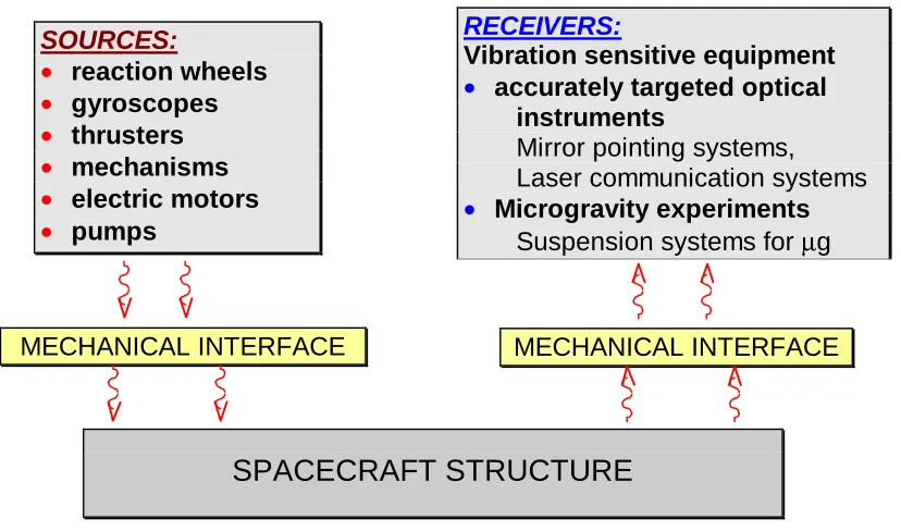
Continuing with a spacecraft as a target application area,, such vibrations are produced by the functioning of on-board equipment such as reaction wheels, gyroscopes, thrusters, electric motors, etc which propagate through the satellite structure towards sensitive equipment (receivers) thereby jeopardizing their correct functioning. Figure 1 shows a schematic illustration of this process.

In practice, the reduction of the vibration level in a structure can be attempted by action at the source(s), receiver(s), and along the vibration path(s). At the source(s), this action consists of attempting to minimize the amplitude(s) of the vibration(s) by, for example, placing equipment on appropriate mountings. The same approach is commonly attempted at the receiver(s) but with the basic objective of sensitivity reduction. Finally, along the vibration path(s), modifications of structural elements or re-location of equipment is attempted with the aim of reducing the mechanical coupling(s) between source(s) and receiver(s).

All of the approaches described are based on so-called passive damping technology and, for routine applica-tions, an appropriate combination of them is often capable of producing the desired levels of dynamic disturbance rejection. The use of active control techniques in such cases would only be as a last resort to achieve desired performance. The requirements of the new generation of satellite based instruments are such that only active control can be expected to provide the required levels of microvibration suppression.

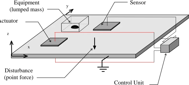
Here we consider the case of a mass loaded panel and a schematic diagram of the arrangement considered is shown in Figure 2. Here the equipment mounted on the panel are treated as lumped masses and the disturbances can be applied in a number of ways, e.g. as a point force in this schematic diagram. For the work reported here, the sinusoidal disturbance is applied via a piezoelectric patch (see Figure 5 below). The sensors and actuators

(2)

[image:2.595.94.508.59.303.2]

Figure 11.1 Propagation path of the microvibrations

SOURCES:

• reaction wheels

• gyroscopes

• thrusters

• mechanisms

• electric motors

• pumps

SPACECRAFT STRUCTURE

MECHANICAL INTERFACE

RECEIVERS:

Vibration sensitive equipment

• accurately targeted optical

instruments

Mirror pointing systems,

Laser communication systems

• Microgravity experiments

Suspension systems for

µ

g

MECHANICAL INTERFACE

Figure 1: Illustrating the propagation path of microvibrations in a satellite structure

employed are twin patches of piezoelectric material bonded onto opposite faces of the panel. The bending vibrations of the panel produce tension and compression of the patches depending on whether they are on the top or the bottom. Due to the piezoelectric effect, these deformations induce an electric field perpendicular to the panel which is detected by the electrodes of the patches. The outer electrodes of the patches are electrically connected together and the panel, which is grounded, is used as the other electrode for both patches of the pair when acting as a sensor. The same configuration is used for an actuator, but in this case the electric field is applied externally to produce compression and tension of the patch, which then induces a curvature on the panel.

The piezoelectric patches were bonded to the panel using epoxy resin. The aluminum panel is glued per-pendicularly on all its four edges to thin metal sheets to ensure a firm support. The thin metal sheets are held by supports attached to a metal base block and the entire structure is suspended on a skeletal frame by four tension springs to provide freely supported boundary conditions to the supporting structure. Figure 3 shows a photograph of the basic experimental arrangement. The reason for having the frame floating is that any attempt to constrain the frame to ground results in flexible modes of the frame being introduced in the frequency range under investigation. This is arbitrarily chosen as 1−500 Hz to include the first 5 modes of the panel. Finally the lumped mass is bonded to the panel. This mass consists of two small solid steel cylinders bonded onto the opposite faces of the panel at the same location and acts as the payload. This arrangement is used in order to maintain symmetry with respect to the middle of the panel and to minimize the moments of inertia of the lumped mass arrangement.

(3)

Actuator

x

y

Control Unit

z

Sensor

Equipment

(lumped mass)

[image:3.595.120.503.85.258.2] [image:3.595.198.429.333.531.2]

Disturbance

(point force)

Figure 11.2 Model layout

Figure 2: Model layout

Lumped

mass Piezoelectric patches

Figure 3: Photograph of the experimental testbed

EM actuators typically generate excitation dominated by a discrete spectrum so the assumptions are realistic from engineering point of view.

In previous work, a range of controllers have been designed and tested. These include linear quadratic Gaussian (LQG) and loop transfer recovery, andH∞ based design methods [2, 1, 6] and require approximating

the dynamics by a finite dimensional state space model and only point disturbance forces were considered. In practice, however, noise and disturbances other than those which cannot be adequately modelled by point disturbances will clearly be present and the major objective here is to develop a control scheme which can deal with these.

(4)

develop-ing and experimentally verifydevelop-ing a control scheme which is capable of estimatdevelop-ing multi-sinusoidal disturbance frequencies and controlling the output signal. The scheme robust in the sense that it is not affected by time do-main modelling errors, which can lead to unacceptable performance when implemented. The reason the scheme developed here is not affected by such errors is that it does not use time domain models and also the frequency domain controller tuning will also be seen to have practically acceptable convergence properties. At the very least, it is an alternative to the well studied adaptive feedforward control algorithms but with the advantages of having feedback action in the control scheme.

This paper is structured as follows. The next section consists of two parts where in the first of these the new control scheme is developed. In the second, the subject is to improve convergence time of the algorithm. The following section deals with frequency estimation on a limited set of data samples. Experimental results are presented and analyzed in Section 5 and finally conclusions are drawn in section 6.

Notation

u - controller input voltage e - accelerometer measurements d - disturbance vibration y - panel acceleration

G - transfer function of approximate plate dynamics ˆ

G - controller gain matrix ˆ

U - controller gain adaptation matrix Jc - instantaneous control cost function

µ - controller adaptation factor ν - panel model adaptation factor Hc - Hessian for controller update Hp - Hessian for panel model update ˆ

g - parameter vector for ˆG ˆ

y - estimate of panel acceleration ˜

d - estimate of disturbance acceleration

2 The New Control Scheme

2.1 Basic Development

The control algorithm presented is a continuation of algorithmic developments in [3, 7, 9]. The novelties in the algorithm introduced here are: (i) the convergence of tuning is improved by the application of inverse Hessians, and (ii) frequency estimation is incorporated into the adaptive scheme.

In Figure 4, a block diagram representation of the system to be controlled is given. The controller aims to minimize the output signaleand the signalε, which is a measure of the error in the plant model. For a perfect output attenuation the control signaluhas to be

u(jωn) =−

d(jωn)

G(jωn), n= 1,· · ·, N (1)

where N is the number of disturbance frequencies to be controlled. The single multi-tone control problem is separated into a set of single tone control problems by using frequency selective filters (FSFs).

In the time domain the algorithm will be based on iterative updating of gain-estimates:

Iterationk Iterationk+1 · · · Iterationk+x Mn Samples Mn Samples · · · Mn Samples

For each disturbance frequency an iterative step consists of Mn samples. A reasonable length for an iterative

step depends on the disturbance frequency and has to be a multiple of the sampling to disturbance frequency ratio. During iterative step k, an LMS estimation results in the complex output gainek(jωn). For simplicity,

(5)

Un

Gn

G^n

T dn + + + -yn Plant with disturbance Controller ^ ~ -~ en en dn ^ Gn un ε εn yn

Figure 4: Block diagram of the system at frequencyn

The criterion for control will be to minimize a quadratic cost function

Jk c def = 1 2e T

kek. (2)

The output can be written in the matrix form

ek=Guk+dk (3)

with

ek def= · ek r ek i ¸

, uk def= · uk r uk i ¸

, gdef=

·

gr

gi ¸

,

dkdef= · dk r dk i ¸

, Gdef=

·

gr −gi

gi gr ¸

(4)

where ek

r and eki denote the real and imaginary parts of ek respectively. The control law will be designed to

update the complex control gainuk+1 into the negative gradient direction of the criterionJck. The gradient of

the criterion function can be calculated as

∂Jk c ∂uk r = ∂e k r ∂uk r

ekr+

∂ek i

∂uk r

eki =grekr+gieki (5)

∂Jk c

∂uk i

= ∂ekr

∂uk i ek r+ ∂ek i ∂uk i ek

i =−giekr+greki (6)

which finally gives

∇Jk

c =GTek. (7)

For the computation of the gradient only an estimate ofGis available. With a design parameterµthe update of the complex gain of the control signal is

uk+1=uk−µGˆ T

(6)

The same adjustment is made to the control path model. The error in the model can be represented by

εk =yk−yˆk= ³

G−Gˆk ´

uk (9)

whereGkˆ is an estimate ofGin (4). Analogous to the controller tuning, the plant cost function is quadratic:

Jk p

def

= 1

2|εk(jωn)|

2

=1 2(ε

k r)2+

1 2(ε

k

i)2 (10)

and the derivations with respect to the plant model parameters are

∂Jk p

∂ˆgk r

=−εkr

∂yˆr

∂gk r

−εki

∂yˆi

∂gk r

=−εkrukr−εkiuki (11)

∂Jk p

∂gˆk i

=εk r

∂yˆr

∂gk i

−εk i

∂yˆi

∂gk i

=εk

ruki −εkiukr (12)

Hence the gradient can be calculated by

∇Jk p =−

·

ur ui

−ui ur ¸ k · εr εi ¸ k

=−Uk˜ εk (13)

and with a design parameterν the plant model can be updated by

ˆ

gk+1=ˆgk+νU˜kεk (14)

and this update of the plant model does not have to be synchronous with the update of the controller coefficients. The design parametersµand ν can be used to tune the algorithm if desired (in the experimental results here they have both been set equal to unity.)

This controller structure has two rates of operation which we detail next:

1. The faster rate, which is equal to the sampling rate, when the controller operates in feed-forward mode, i.e. there is no feedback with the batches.

2. A slower rate of operation for the estimation of the complex gains based on batches of data. At this slower rate there is feedback action to tune the complex amplitudes of the feedforward input signal. As the control input is updated based on the output signal, this is feedback control action.

Since there is no reference or detection signal that the control scheme could rely on, it is clearly a nonlinear feedback scheme at the slower rate, i.e. with a dead-zone equal to the length of a batch.

2.2 Improved convergence time

It can be shown that the control algorithm presented in the previous section is stable and converges [4], but this can take a long (in relative terms) time. It also has to be decided how to select the adaptive gainsµandν for optimal convergence. There is an easy and efficient way to increase the convergence speed using the inverse Hessian matrix [8]. This also avoids the problem of choosing suitable adaptation gains for convergence and is detailed next, where first the inverse Hessian matrix is derived for the control parameter update.

The Hessian is calculated as

Hk c =

·

ˆ gT

kˆgk 0

0 ˆgT kgˆk

¸

(15)

and its inverse as

H−1 c =

1 ˆ gT

kˆgk

·

1 0 0 1

¸

(7)

Hence the control signal in (8) can be updated as

uk+1=uk− 1

ˆ gT

kgˆk

ˆ

GT_kek. (17)

The Hessian with respect to the plant model parameters is calculated to be

Hk p=

·

uT

kuk 0

0 uT kuk

¸

(18)

and the inverse is given by

H−1 p =

1 uT

kuk

·

1 0 0 1

¸

. (19)

Hence, the plant model (14) can be updated as

ˆ

gk+1= ˆgk+ 1

uT kuk

˜

Ukεk (20)

These two update equations (17) and (19) are easy to implement and, in particular, no extra signal calculations are required.

3 Frequency Estimation

Most previous work on algorithms such as that of the previous section assumes a prior knowledge of the disturbance signal d, or that measurements are taken separately. Here as a new development, a frequency estimator is proposed for use before the complex gain estimation step and is termed optimized frequency estimation (OFE).

An initial estimation of the disturbance peaks can be obtained by applying the FFT. For a fixed number of samplesS, the FFT can, however, only produce a resolution, which equals the sampling frequencyfsto number

of samplesSratio. Therefore, true frequencies will be drawn to their nearest representative frequency depending onfs andS. This information on the ’rough’ frequencies present will be used to determineN bandpass filters

for the FSF scheme where the following frequency estimation algorithm is applied. The recorded output signal, without using control is

e(t) =d(t) (21)

and, in essence, the frequency estimate is calculated by using a nonlinear least mean squares method. To describe this method, assume a sum of periodic N sinusoids of the form below is present in the disturbance signal and measured at the output

e(t) =

N X

n=1

[ansin (ωnt) +bncos (ωnt)] +ρ (22)

withan andbnbeing the true coefficients andρsome minor noise. Given the rough locations of the disturbance

frequencies, the output signal is filtered, using FSFs for each relevant frequency, to obtain a set of signals consisting of only one frequency and some minor noiseρn. The filtered output signal at frequency ωn can be

written as

en(t) = £

sin(ωnt) cos(ωnt) ¤· _a_n

bn ¸

+ρn

where the realωn is unknown and is to be estimated. Introduce the vector

z(t,ωˆn) = £

sin(ˆωnt) cos(ˆωnt) ¤

(8)

and define the matrixZn as

Zn= 

 

z(t0,ωˆn)

.. . z(tf,ωˆn)





 (24)

where t0 to tf determine the chosen range of sampling points to avoid the filter transient effects. Therefore,

the output signal vector is given by en= £

en(t0) . . . en(tf) ¤T

and the complex gain coefficients can be calculated by a least mean squares estimation

·

ˆ a(ˆωn)

ˆ_b_(ˆ_ω_n₎

¸

=³ZT nZn

´−1

ZT

nen. (25)

The evaluation of the estimated frequency, ˆω, obtained by minimizing the mean-square error between the true and estimated frequency within the range of sampled points, is given by

Figure 5: Schematic diagram of satellite panel experimental setup.

r(t,ωˆ) = arg min

ˆ

ω "µ

en−Zn

·

ˆ a(ˆωn)

ˆ b(ˆωn)

¸¶Tµ

en−Zn

·

ˆ a(ˆωn)

ˆ b(ˆωn)

¸¶#

.

Repeating the procedure defined by(23)–(26) for each of the frequencies, ωn, the residual signal r(t,ωˆn) can

be calculated by taking the difference between the disturbance signal and the corresponding estimated signal. Each value of the new estimated frequency ˆω derived fromr(t,ωˆn) can be used to calculate a complex output

gain of measured data for control use.

4 Experimental Validation

Figure 5 is a schematic of the experimental test-bed used to obtained the results given in this section. (In effect, this is Figure 3 augmented by the hardware and software necessary to perform the tests reported in this section and with the disturbance applied through a piezoelectric patch.) The objective is to minimize the plant error function so as to cancel out the disturbance vibration. Inaccurate frequencies estimates tend to instability even with a robust adaptive control system. For this particular programme of experiments, the piezoelectric output sensor is positioned at the location where attenuation is intended and the control piezoelectric actuator directly beneath it on the opposite face of the aluminum panel. The natural frequencies of the plate are listed in Table 2.

(9)

Table 1: The natural frequencies of the plate with and without the patches. Mode Bare panel Panel with patches

1,1 125.3 125.0

2,1 240.5 238.5

1,2 383.9 383.0

3,1 431.5 432.5

2,2 499.0 487.5

controller signals are amplified by an electronic amplifier separately (LM1875 at gain=4.9 and LM1876 at gain=2 respectively) before each excites a piezoelectric actuator. The piezoelectric sensor is located at the actuator, converting mechanical vibrations to electrical signal, before feeding it back to the workstation for control. Co-location of the actuator and sensor improves control performance but does not make the problem any easier for this type of control scheme, which is clearly applicable in the presence of non-collocated sensor-actuator pairs. All channel signals are displayed on oscilloscopes to monitor the signals status. Signals are filtered before transmission or after vibration reception. A bandpass filter is used to filter out the low frequency from the power mains and higher noise frequencies. Lowpass filters are used by the actuators to eliminate the effect of zero order hold components at the output of the D/A channel.

A sum of three dominant disturbance frequencies was generated at 133.3334Hz, 190.4762Hz and 285.7143Hz (correct to 4 decimal places). The disturbance spectrum received by the sensor is estimated by the OFE method. Estimated frequencies are used by the controller algorithm which will produce an anti-phase vibration cancellation at the controller patch.

Figure 6(a) shows the disturbance time series signal for 0.1 second (where the vertical axis in this and the next set of plots is referenced to the voltages at the patches). For comparison, the FFT and OFE methods are compared to highlight the stability of the latter, where the corresponding results are shown in Figures 6(b) and 6(c) respectively. The disturbance frequencies estimated by FFT for signal to noise ratio SNR=40 have values of 134, 190 and 286Hz respectively. The OFE method estimated the disturbance frequencies as 133.3319, 190.4732, and 285.7071Hz respectively for a SNR=40. The FFT-estimated frequencies are sufficiently different from their true values with the result in the controller cannot converge to minimize the cost function, leading to an unstable system. The corresponding frequency domain plots of the disturbance signal, unstable FFT and attenuated signal by OFE are given in Figures 7(a) to 7(c) respectively. Note the difference in the y-axis scales.

These plots clearly confirm that the three dominant tones are attenuated until near the level of the system measurement noise. The total power attenuation using OFE method is calculated to be 26dB. It is common to find that most real signals are corrupted by a certain level of noise which can be caused by various sources, such as the quantization, anti-aliasing filtering, background noise and imperfect instrument responses, e.g. actuators. Figure 8 shows the total power attenuation across different noise levels.

Generally, OFE-estimated frequencies attenuate the disturbance signal with increasing SNR. This is to be expected as more accurate frequency estimates contribute to better attenuation. Conversely, FFT-estimated frequencies produce unstable systems such that the total signal power is even higher than the disturbance signal itself. For SNR<0, which is here taken to be a system with significant noise corruption, the OFE method developed here gave very similar signal power as the disturbance signal and hence no discernible attenuation. The attenuation is more significant from SNR>0 onward where increasing the SNR gave even higher attenuation. Table 2 shows the estimated frequencies of the disturbance signal for the two estimators under increasing noise levels and their stable/unstable property. The table indicates that an FFT estimation is not good enough for control. The frequencies are shown up to 7 significant figures as these are important when controlling vibrations with a feed-forward scheme such as the one described here, since error in frequency estimation causes deterioration of performance. The high level of attenuation was achieved largely due to these accurate frequency estimates.

(10)

(a) Disturbance signal.

(b) Unstable signal of FFT-estimated frequencies.

(c) Attenuated signal of OFE-estimated frequencies.

Figure 6: Time domain signals at SNR=40.

5 Conclusions

This paper has developed a control scheme which estimates multi-sinusoidal disturbance frequencies acting on a system and controls the output signal. In particular, the control of microvibrations has been considered, where one possible end application for the outcome of basic the basic research considered here is panel structures on nano-satellites. The algorithm itself results in a controller which has two rates of operation where the faster of these is equal to the sampling rate where the controller operates in feed-forward mode, i.e. there is no feedback from the batches of data generated. The slower rate of operation is used to estimate the complex gains based on batches of data. At this slower rate there is feedback action to tune the complex amplitudes of the feedforward input signal. As the control input is updated based on the output signal, this is feedback control action and overall the scheme is of the feedforward/feedback type and hence opens up on means of obtaining the beneficial effects of both. The predicted performance from the resulting algorithm has been experimentally verified on a specially constructed laboratory testbed and the results obtained clearly demonstrate the effectiveness of the scheme.

(11)

(a) Disturbance frequency domain signal.

(b) Unstable signal in frequency domain after using FFT-estimated frequencies.

(c) Attenuated disturbance signal in frequency domain after using OFE-estimated frequencies.

Figure 7: Signals in frequency domain at SNR=40.

Acknowledgement

This research work is supported by EPSRC grant GR/N32297/01.

References

[1] G. S. Aglietti. Active control of microvibrations for equipment loaded spacecraft panels. PhD thesis, School of Engineering Sciences, University of Southampton, UK, 1999.

[2] G. S. Aglietti, S. B. Gabriel, R. S. Langley, and E. Rogers. A modeling technique for active design studies with application to spacecraft microvibrations. The Acoustical Society of America, 102:2158–2166, 1997.

[3] T. Meurers and S.M. Veres. Further results on the iterative design for noise attenuation. International

Journal of Acoustics and Vibration, 6(4):219–225, 2001.

[4] T. Meurers and S.M. Veres. Stability analysis of secondary path estimation during FSF-based feedback control. Proc. CCA 2002, Glasgow, CD-Rom, 2002.

(12)

Figure 8: Total signal power of 3 dominant frequencies for disturbance, Q&F and OFE methods.

[6] J. Stoustrup, G. S. Aglietti, E. Rogers, R. S. Langley, and S. B. Gabriel. H∞controllers for the rejection of

microvibrations. Proceedings European Control Conference (ECC99), pages CD–Rom proceedings, 1999.

[7] O. Tokhi and S.M. Veres. Active Control of Sound and Vibration. IEE Peter Peregrinus, London, 2001.

[8] H. Unbehauen. Regelungstechnik III. Vieweg, Braunschweig, 1985.

(13)

Table 2: Estimated frequencies of the disturbance signal with various estimating methods and SNRs. FFT OFE True Freq

SNR=-20 134Hz, 190Hz, 286Hz (unstable)

133.4323Hz, 190.1451Hz, 285.9376Hz (stable)