Prediction Markets for Machine Learning: Equilibrium Behaviour through Sequential Markets

(1)

Prediction Markets for Machine

Learning: Equilibrium Behaviour

through Sequential Markets

Franciscu Hettige Anne Mindika

Premachandra

A thesis submitted for the degree of

Doctor of Philosophy

The Australian National University

(2)

c

(3)

Except where otherwise indicated, this thesis is my own original work.

(4)

(5)

Acknowledgements

It is with deepest appreciation I wish to express my special thanks to all those who helped me in many ways to complete my research training and this thesis.

A very special thanks to my supervisor, Dr. Mark D. Reid, for the valuable advice, collaboration, hours of discussion, comments and reviews, he offered me generously.

Special thanks to my panel chair, Prof. Bob Williamson, for his inspiration, words of advice and guidance.

Furthermore, I would like to thank with much appreciation, the Australian National University for granting me a scholarship to pursue this research and the NICTA (Na-tional ICT Australia) for providing a valuable research environment and financial support.

I also take this opportunity to thank the University of Colombo School of Computing (UCSC) for granting me study leave to undertake this research and I wish to express my deepest gratitude to my teachers at UCSC, specially Dr. Lalith Premaratne for guidance and endless support throughout my student life and academic career and Dr. Ruvan Weerasinghe for introducing me to research.

A special thanks to my family for their affection, love and guidance showered through-out my life and the prayers offered for me.

Finally, I would like to express my appreciation to my beloved husband Chamara for his continuous support and encouragement. Last but not least I recall with much love my son Tharun Angelo for his contribution in his own little way and my lit-tle baby daughter Anne Tharundee for coming into my life during the end of this rewarding journey.

(6)

Abstract

Prediction markets which trade on contracts representing unknown future outcomes are designed specifically to aggregate expert predictions via the market price. While there are some existing machine learning interpretations for the market price and connections to Bayesian updating under the equilibrium analysis of such markets, there is less of an understanding of what the instantaneous price in sequentially traded markets means. In this thesis I show that the prices generated in sequen-tially traded prediction markets are stochastic approximations to the price given by an equilibrium analysis. This is done by showing that the equilibrium price is a solution to a stochastic optimisation problem which is solved by stochastic mirror descent (SMD) by a class of sequential pricing mechanisms. This connection leads to proposing a scheme called “mini-trading” which introduces a parameter related to the learning rate in SMD. I prove several properties of this scheme and show that it can improve the stability of prices in sequentially traded prediction markets.

Also I analyse two popular trading models (namely the Maximum Expected Util-ity model and the Risk-measure model) in respect to an assumption on the class of traders I required to interpret sequential markets as SMD. I derive a sufficient con-dition for when the Maximum Expected Utility traders satisfy this assumption, but show that risk-measure based traders naturally satisfy this assumption for the type of markets I consider. Then I show that the “regret” of mini-trading markets (with respect to equilibrium markets) depend on the mini-trade parameter.

Finally I attempt to compare the wealth updates of traders in sequential markets to the wealth updates in equilibrium markets, since this would help to extend the interpretation of equilibrium markets as performing Bayesian updates to sequential markets. For this I present preliminary results.

(7)

List of Figures

2.1 Screen-shot of an Intrade’s market (from [Pennock, 2010]) . . . 23 2.2 Market Maker Equivalence Relations (Diagram from [Chen and

Pen-nock, 2007]) . . . 29

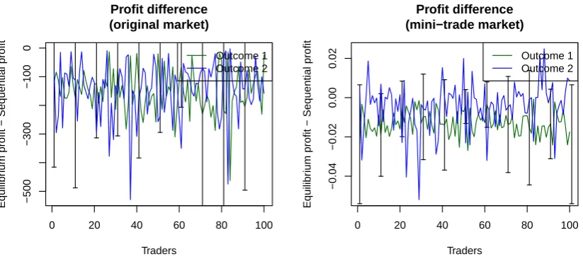
3.1 The price history of full-trade and mini-trade markets, averaged over 30 simulations. The dashed line marks the equilibrium price and bars show standard deviation. . . 49 3.2 The profit differences of traders in full-trade and mini-trade markets,

averaged over 30 simulations. Bars show standard deviation. . . 50

(11)

List of Tables

2.1 Proper Scoring Rule Examples [Hanson, 2007] . . . 24

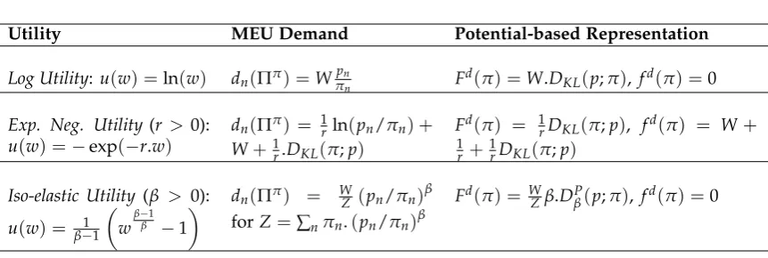
3.1 Potential-based MEU demands for beliefs p∈_∆N_{, wealth}_W_{and prices} π ∈∆N . . . 41

4.1 MEU solutions for HARA utilities and connections to divergences . . . 63

(12)

Chapter1

Introduction

1 .

1 Thesis Statement

Both equilibrium markets and sequential cost function based markets can be inter-preted as solutions to the same learning problem in terms of the market price, thereby naturally extending the existing interpretations of equilibrium markets as perform-ing known aggregations to sequential markets. I also give preliminary results that relate the wealth updates of traders in equilibrium markets to sequential markets, which would extend the existing interpretations of equilibrium markets as perform-ing Bayesian updatperform-ing to sequential markets.

1 .

2 Introduction

The main purposes of prediction markets are eliciting and aggregating beliefs over an unknown future outcome. Traders with different beliefs trade on contracts whose payoff’s are related to an unknown future outcome and the market prices of the con-tracts are considered as the aggregated beliefs. While machine learning aggregation models (such as boosting) perform aggregations over expert beliefs or machine learn-ing models, prediction markets can be used to appeal to the wisdom of the crowds [Surowiecki, 2004] and may also be used to aggregate expert/model beliefs with hu-man judgement. But unlike in machine learning algorithms where expert beliefs are readily available for aggregation, traders in a prediction market may have to be in-centivised to participate in the market.

One feature of most of the machine learning aggregation methods including boost-ing and hedgboost-ing is the combination of multiple homogeneous models (i.e., models of the same type) for aggregation (in boosting and hedging, the set of predictors are obtained by using the same weak-learning algorithm iteratively). But prediction markets have the capability to work with traders who have diverse information and

(13)

§1.2 Introduction 2

diverse decision making models, so prediction markets can also be used to imple-ment generalised aggregations.

Recently many connections between prediction markets and machine learning have been shown based on the (Walrasian) equilibrium analysis. Storkey [2011] and Storkey et al. [2012] show how well-known aggregation techniques including ma-jority voting (mode), simple averaging (mean) (in random forests [Breiman, 2001]), weighted-mean (in AdaBoost [Freund and Schapire, 1995]), median, weighted-median, mixtures of experts [Jacobs et al., 1991] can be re-created in prediction markets. Beygelzimer et al. [2012] show connections to Bayesian updating for markets with Kelly bettors [Kelly, 1956], which Storkey et al. [2012] generalise for a more wider class of traders. Lay and Barbu [2011] show how different trading behaviour can lead to implementing weighted averaging, kernel methods, logistic regression in prediction markets. Although these connections present nice interpretations of pre-diction markets in a machine learning point of view, more often the equilibrium analysis does not provide a closed-form solution and pre-suppose some kind of off-equilibrium trading process that eventually converges to a point whose properties are studied.

Sequential markets, where traders act in sequence, have been widely adopted in practice. For the purpose of this thesis I adopt a type of market with anAutomated Market-Makerwhere traders are only allowed to trade with a central market maker in a sequential fashion (typically at the price that is determined by the market-maker). Chen and Pennock [2007] show that Sequential Cost Function based Markets (which is the type of sequential market I consider in this thesis) have connections to the popular Market Scoring Rules by Hanson [2007] which uses a Proper Scoring Rule to reward participants based on their reports. Chen and Vaughan [2010] show con-nections to follow-the-reguralized-leader/ no-regret algorithms using cost function based markets. Further connections with weight updates of experts in follow-the-reguralized-leader algorithms and price updates of contracts in sequential cost func-tion based markets have been shown by Abernethy et al. [2011]. Even though there are well specified price update mechanisms for sequential markets, the market dy-namics become difficult to analyse due to the sequential nature of trading.

(14)

§1.3 Original Contributions 3

by interpreting the price updates of sequentially traded markets as Stochastic Mirror Descent (SMD) and then interpreting its equilibrium as solving the same optimi-sation problem, thus establishing a connection between sequential and equilibrium market prices. The closest work to this result is by Frongillo et al. [2012] who first interpreted sequential markets as performing a SMD and established a connection between sequential markets and equilibrium analysis using limiting conditions on sequential markets. The interpretation of sequential markets as SMD in this thesis is a variation of their result for a more broader class of trades and a more restrictive class of markets. Further this thesis establishes a connection between sequential mar-kets and equilibrium without using limiting conditions.

I then introduce mini-trading as a mechanism for implementing the learning rate parameter that is used for convergence in SMD. Also I analyse two popular trading models (namely the Maximum Expected Utility model and the Risk-measure model) in respect to the assumption on the class of traders I required to interpret sequential markets as SMD.

Finally I attempt to compare sequential and equilibrium markets in terms of traders’ wealth updates, since equilibrium markets have been shown to implement Bayesian wealth updates for traders. For this I obtain preliminary results.

1 .

3 Original Contributions

While the classical market analysis techniques (i.e., the Walrasian equilibrium) has been shown to implement known machine learning aggregations and performing generalised Bayesian updating, there is less of an understanding of what the instan-taneous price in sequentially traded markets means and how the traders’ wealth updates compare with the equilibrium setting.

The main contributions of this thesis are,

• Interpreting the instantaneous price of sequential markets as stochastically

min-imizing (via stochastic mirror descent(SMD)) the same objective as its Wal-rasian equilibrium, thus unifying the meaning of instantaneous and equilib-rium prices via an optimisation point of view (for markets and traders satisfy-ing certain conditions).

• Designing “mini-trading” as a mechanism for implementing the learning rate

(15)

§1.4 Thesis Outline 4

is to allow repeated but small-scale trader interactions as opposed to single but large-scale interactions in a sequential market, also resulting in more stable prices and bounded worst-case loss.

• Showing that the Maximum Expected Utility trader model does not always

satisfy the conditions needed for the SMD interpretation. But the analysis pro-vides a sufficient condition in which this is satisfied.

• Showing that the risk-measure based trader model satisfies the conditions needed

for the SMD interpretation.

• Showing that the “regret” of mini-trading markets (with respect to equilibrium

markets) depend on the mini-trade parameter.

• Showing that the total of traders’ wealth updates in mini-trading sequential

markets are not far off from the total equilibrium wealth updates, which are preliminary results to relate sequential wealth updates with equilibrium wealth updates.

1 .

4 Thesis Outline

First I introduce prediction markets and briefly discuss how prediction markets and traders resemble machine learning aggregations and experts/models that are used in machine learning aggregations in Section 2.1. Here I also discuss contracts in prediction markets and how traders make demands (purchases) based on contract pricing depending on their trader model (e.g., maximum expected utility model, risk-measure based model). In Section 2.2, I describe the (Walrasian) equilibrium model and its connections to machine learning aggregations. Then in Section 2.3, I discuss sequential markets and focus on the type of sequential market that is con-sidered in this thesis (namely cost-function based sequential markets) and discuss its connections to machine learning methods. Then I discuss the importance of making connections between equilibrium and sequential markets which have their own sep-arate connections with machine learning and discuss the existing work in this area (Section 2.4), and also discuss how the main contribution of this thesis (i.e., relating sequential and equilibrium prices in Chapter 3) compares and differs from existing work. I also briefly describe the interpretation of equilibrium wealth updates as Bayesian wealth updates in Section 2.5, which motivates Chapter 5.

(16)

§1.5 Publications and Collaborations 5

contribution I briefly introduce the two types of markets we consider (Section 3.1) and present concepts related to convex analysis (Section 3.2) which makes it possible to interpret the stochastic price update of sequential markets via stochastic mirror descent. Section 3.3 starts by giving the assumptions on the markets and trader demands and Theorem 1 interprets the instantaneous price of sequential markets as stochastically minimizing (via stochastic mirror descent (SMD)) the same objec-tive as its Walrasian equilibrium, thus unifying the meaning of instantaneous and equilibrium prices via an optimisation point of view. The mini-trading mechanism introduced in Section 3.4 can be seen as a mechanism for implementing the learning rate parameter that is used for convergence in SMD. Then we show that mini-trading has desirable properties like more stable prices (Theorem 2) and bounded worst-case loss.

In Chapter 4, I analyse two popular trader models with respect to the assump-tion we made on trader demands (i.e., the potential-based assumpassump-tion defined in Section 3.3.2) that makes it possible to interpret sequential pricing as SMD. The Maximum Expected Utility trader model is considered in Section 4.1, which gives a sufficient condition for potential-based demands (see Collorary 1 following The-orem 3). The Risk-measure based model is considered in Section 4.2, resulting in potential-based demands in particular trading scenarios (see Theorem 4). Section 4.3 obtains regret bounds for mini-trading sequential markets with potential based de-mands with respect to equilibrium markets.

Chapter 5 presents preliminary work (Theorems 5 and 6) which compares the wealth updates of traders with potential based demands in mini-trading sequential markets with the wealth updates in equilibrium markets.

Finally, I present conclusions and future work in Chapter 6.

1 .

5 Publications and Collaborations

(17)

Chapter2

Background and Related Work

Here I will motivate the study of markets from a machine learning perspective and introduce the notions of traders, contracts, prediction markets, equilibria, and se-quential market making. After contrasting ensemble methods and market mecha-nisms, I will discuss the existing work on understanding the behaviour of equilib-rium and sequential prediction markets and their ability to aggregate agent beliefs, I will argue that the relationship between these two kinds of markets is not well under-stood, which is the focus area of this thesis. Central to the relationship given as the main contribution of this thesis (presented in Chapter 3) is understanding models of trader demand as it is the common link between the two types of markets. I briefly review two existing models (Maximum Expected Utility and risk-based traders) that are explored further in Chapter 4. Finally, I survey what is known about the dynam-ics of repeated equilibrium markets (and relationships with ML) and point to some of my results and open questions in Chapter 5 about repeated sequential markets.

2 .

1 Prediction markets

After a broad introduction to prediction markets, I discuss the similarities and dif-ferences of prediction markets and ML ensemble methods in Section 2.1.2. I also discuss contracts and their pricing in Section 2.1.3, and finally how trader behaviour is influenced by trader models, beliefs and reaction to prices, etc. in Section 2.1.4.

2.1.1 Introduction to prediction markets

A market is a structure that allows buyers and sellers to exchange goods, services or information. They vary in size (physical retail markets, shopping complex, com-modity markets), location (village, town, local, national, international, web-based), trading mechanism (barter, fixed price, bidding, auctions) and by what is traded. Markets also provide direct and indirect information about the price, demand,

(18)

§2.1 Prediction markets 7

ability, stakeholders and can be used to identify patterns, trends and formulate be-liefs. Financial markets (e.g., stock markets, bond markets, futures markets, currency markets, money markets) which facilitate the exchange of liquid assets are widely used for speculation on company stability, financial risk, price changes, exchange rates, etc. This ability of markets emerge from the participants and stakeholders who influence the market prices, demand and availability through various means such as holding exclusive information, wealth, capacity of production (or number of shares, betting instances available), regulations and even by illegal and unethical means.

The price of a certain asset in a stock market at a given time, which is the result of the set of market interactions that occurred and each participant’s private valua-tion of the asset, is normally a good indicavalua-tion of the expected benefit from holding that asset. Likewise, there is evidence to suggest that the consensus belief of a group of individuals with heterogeneous beliefs can give better results than a group of in-dividuals with heterogeneous beliefs, the consensus belief of all might give better results than taking the advice of a single individual [Surowiecki, 2004]. Then comes the questions of how to aggregate the information and whether the individuals are genuinely interested in helping to form a better opinion. This is also a problem in

crowdsourcing [Howe, 2006], which is a distributed problem-solving and production model. Other approaches which address information aggregation are the ensemble methods in machine learning and game-theoretic methods.

Financial markets are usually created to allow traders to hedge risks and with the ex-istence of speculators who seek to make a profit from the current prices. Speculative market prices often become a good estimate of future prices, being able to aggregate a great deal of information in the market price [Hanson, 2003]. While this feature of price discovery through information aggregation is a side effect of financial markets, prediction markets (also called information markets or event futures) are designed specifically to aggregate information on particular topics of interest [Chen and Pen-nock, 2007; Wolfers and Zitzewitz, 2004; Arrow et al., 2008].

(19)

betting and sometimes even among themselves.

Considering a set of N base events, where each event n has Vn different possible

values or values in a continuous range, there can be different measures that a predic-tion market can be interested in predicting. For example, we might want to predict the probability of each event, or the joint probabilities, event conditional probabili-ties, expected values, medians, percentiles, etc. Typical prediction markets that we see today are interested in predicting one or just a few of measures and mostly con-sist of binary events or one event with a continuous value range. Some examples of real-world prediction markets are given below. This shows that prediction mar-kets are used in many domains (including elections, sports, business, economics and entertainment industry).

Iowa Electronic Markets (IEM) : (tippie.uiowa.edu/iem/) Run by the University of Iowa as an educational and research project, the IEM is a small-scale real-money online futures market where contract pay-offs are based on real-world events such as political outcomes, companies’ earnings per share (EPS), and stock price returns. For most future events (like the U.S. Presidential Elections), they run two separate markets, a “winner-takes-all” market for predicting a future event with discrete but mutually certain outcomes (e.g., the Winner-Takes-All Market to predict whether the Democratic Party nominee or the Republican Party nominee will receive the popular vote), and for predicting the value of a continuous variable (e.g., Presidential Vote Share Market to predict the vote share percentage received by the two parties). A similar election market is run by the University of British Columbia (http://esm.ubc.ca/forecast.php).

TradeSports : (www.tradesports.com) Was originally a real money market which traded in a rich set of political futures, financial contracts, current events, sports and entertainment. Now operates basically as a virtual money market which offers pre-game and real-time trading for sports events.

Intrade : (www.intrade.com) Used to be a real-money market that allowed to make predictions on the outcome of binary events using "winner-takes-all" contracts based on real-world events. Some example markets: The Dow Jones to close on or above 13,000 on 30 Dec 2012, Barack Obama to be re-elected President in 2012, The United States or Israel to bomb Iran before the end of 2013.

(20)

prediction market solutions for the business realm.

Economic Derivatives : (www.economicderivatives.com) A large scale real-money mar-ket run by the Goldman Sachs and Deutsche Bank for trading in the likely out-come of future economic data releases such employment, retail sales, industrial production and business confidence.

Hollywood Stock Exchange : (www.hsx.com) A play money market which predicts the success of movies, movie stars, awards, including a related set of complex derivatives and futures.

For more examples for the wide range of applications and success stories of predic-tion markets see Arrow et al. [2008]; Wolfers and Zitzewitz [2004].

Prediction markets can be thought of as belonging to the more general concept of

(21)

2.1.2 Agents, Trading, and Aggregation

Here I will discuss the similarities and differences of prediction market aggregation with ensemble methods and motivate why prediction markets may be used for ag-gregation instead of traditional machine learning ensembles. Similar motivations are discussed in Storkey [2011].

The main aim of the prediction markets mechanisms we consider is to produce a probability π ∈ ∆N representing some “consensus belief” of the market about the

future outcome. Such a mechanism is loosely analogous to an ensemble for a multi-class probability estimation problem in the machine learning literature (e.g., boost-ing, random forest aggregations) which aggregates the predictions of several base predictors.

In a prediction market, traders may be viewed as the base predictors and their be-liefs may not be directly available as in ensemble methods. Traders interact with the market via purchasing contracts, instead of directly submitting their beliefs. Now consider a machine learning aggregation where the base predictors are reluctant to submit their beliefs for free. Then the need arises to incentivise the base predic-tors to reveal their information. Prediction markets naturally provide incentives for participation by the sale of contracts, generally designed to elicit information from participants (see the discussion on Market Scoring Rules in Section 2.3.2) and are said to aggregate traders beliefs in to the market price. So prediction markets can be used for machine learning aggregations where the base predictors are reluctant to submit their beliefs. By setting up a machine learning aggregation as a prediction market, we could also invite more participants (humans or machine learning mod-els) to contribute to the aggregation, thus being able to appeal to the wisdom of the crowds as in crowdsourcing.

(22)

2.1.3 Contracts and Prices

Here I describe the Arrow Debreu securities [Arrow and Debreu, 1954] and how it relates to aggregating trader beliefs/probabilities about future events. For complete-ness, I also give a brief description of other types of contracts. Since traders generally consider the pricing of contracts when trading, in Section 2.1.3.1 I formalise and give examples of some pricing functions used in prediction markets.

In order to use a prediction market to predict the outcome of a future event, the type of contracts that is being traded plays an important role. Awinner-takes-all con-tract costs some amount $p and pays off a fixed amount (e.g.: $1) if and only if a specific event occurs, like a particular candidate winning an election. The price of a winner-take-all market represents the market’s expectation of the probability that an event will occur (assuming risk neutrality) [Wolfers and Zitzewitz, 2004] (e.g., 2012 US Presidential Election Winner-Takes-All Market in IEM).

The Arrow-Debreu security is the simplest type of contract in prediction markets for classification. It pays one unit of the traded currency ($1) if a particular state of the world is reached and zero otherwise, and is therefore a "winner-takes-all" type of contract. Since we are interested in mechanisms for aggregating trader beliefs about a single future event with N of possible outcomes, we consider prediction markets where the “goods” that are traded are N types of contracts – one for each of the N

outcomes – that pay $1 if outcomen∈ [N]occurs and nothing otherwise.

Although the Winner-takes-all or Arrow-Debreu contracts are generally used for ag-gregating predictions in the form of probabilities, Lay and Barbu [2011] showed how Arrow-Debreu contracts can be used in “artificial” prediction markets (that attempts to mimic a real prediction market in a machine learning setting) for implementing weighted-mean aggregation, logistic regression and some kernel methods by artifi-cially controlling how much traders spend on each outcome. See Lay and Barbu [2012] for use of “artificial” prediction markets for regression (where there are un-countably many possible outcomes) using contracts whose payoff depends on a re-ward kernel that rere-wards contracts based on the distance to the ground truth value.

(23)

one that pays according to the square of the indexy, the market prices will reveal the market’s expectation of E[y2_]_{(e.g.: 2012 US Presidential Vote Share Market in IEM).} [Wolfers and Zitzewitz, 2004]

Also see Abernethy et al. [2011], Abernethy et al. [2013] for a generalised frame-work for contracts with arbitrary payoff functions and for the design of securities markets over combinatorial or infinite state or outcome spaces. For introduction to combinatorial prediction markets, see Hanson [2003] and Chen et al. [2008].

The remainder of this thesis will focus only on Arrow-Debreu contracts.

2.1.3.1 Contract pricing

I will use the following notation. The set {1, . . . ,N} will be written as [N] and

∆N := {π ∈ [0, 1]N :hπ,1i=1}will denote the set of probability distributions over

[N]. Given vectorsx,y∈RN_{, their inner product will be denoted}_h_x_,_y_i_:₌_∑N n=1xnyn

and we use 1 := (1, . . . , 1) ∈ RN _{to denote the vector of all ones. For a}

dif-ferentiable function C(x) : RN → R, its derivative at x ∈ RN _{will be written}

∇C(x):= ∂C_∂x(x)

1 , . . . ,

∂C(x)

∂xN

.

A common form of trading in markets is based on the assignment of prices to goods. Since the goods we consider are the contracts on future events, I will useΠ:RN →_R to denote apricing functionthat assigns a price Π(s)to each contract bundle s ∈ RN_.

Each component sn represents the (possibly fractional) number of contracts bought

for outcome n ∈ [N]with sn < 0 representing a sale of−sn contracts. P is used to

denote the set of pricing functions.

A very simple form of pricing function is one that assigns a fixed priceπn per unit

contract for outcomen, whereπ ∈ ∆N. The price for a bundles ∈ RN is then given

byΠπ₍_s₎_:₌_h

π,si, which will be called afixed-pricepricing function.

Another type of pricing function that is used when sequential markets are consid-ered is acost function-based pricing function. A cost function-based pricing function is defined by

ΠC,x₍_s₎_:₌_C₍_x₊_s₎₋_C₍_x₎_.

(24)

charges the difference between the value at positionx(which denotes the total num-ber of contracts sold so far) and the value if the position was moved to x+s. The value of∇C(x)can be seen as the price for buying an infinitesimally small bundle at positionx and is therefore called theinstantaneous priceatx.

One of the most well studied cost function-based pricing functions used in predic-tion markets is the Logarithmic Market Scoring Rule (LMSR) [Hanson, 2007]. This is defined by the cost functionC(x) =blog_∑_nN₌₁exp(xn/b)

whereb>0 is some-times called theliquidity parameter. The LMSR has instantaneous prices (∇C(x))_n=

Z−1_exp₍_x

n/b)whereZ =∑Nn=1exp(xn/b).

2.1.4 Traders and Demands

I assume that traders make purchases (demands) considering their own beliefs, prices, etc. depending on the trader model. The work on interpreting sequential markets as Stochastic Mirror Descent (SMD) and the relation to equilibrium markets in Sec-tion 3.3 is based on traders making demands satisfying a certain condiSec-tion called

potential-based demandsdefined in Section 3.3.2.

A trader’s purchasing behaviour will be modelled through a demand operator d that reacts to pricing functions. Formally, d : P → RN _{will return a contract bundle} d(Π) ∈ RN _{when given a pricing function} _Π_{∈ P}_{. The returned bundle represents}

the contracts the trader wishes to buy when bundles are priced according to Π. In the case of fixed-priced pricing (i.e.,Ππ_{), I abbreviate the demand operator}_d₍Ππ₎_to d(π).

Next I briefly introduce two existing models (MEU and risk-based) that are com-monly used in prediction markets. These are explored further in Chapter 4. For completeness I also briefly mention risk-neutral traders. Also see Lay and Barbu [2010, 2011, 2012] where traders’ demands are defined using a “betting function” which specifies what percentage of its budget/wealth the trader will allocate to pur-chase contracts for each contract.

2.1.4.1 Maximum Expected Utility (MEU) traders

A common assumption about traders is that they are risk averse expected utility max-imisers. That is, their demands are determined by theirbelief p∈ ∆N_,_{wealth W}_∈ _R_,

(25)

for a guaranteed $1₂(x+y)is always larger than their expected utility for a coin toss resulting in $x or $y. They also exhibitdiminishing marginal utility of wealth, which means that there is a decline in the marginal utility that person derives from each additional unit of wealth (or that the first unit of wealth yields more utility than the second and subsequent units).

MEU trader model has been widely used in the prediction market literature. Exam-ples include those by Beygelzimer et al. [2012], Wolfers and Zitzewitz [2006], Storkey [2011], Storkey et al. [2012], Sethi and Vaughan [2013], that will be discussed in Sec-tions 2.2 and 2.4. Market mechanisms have also been derived using the expected utility framework (see Chen and Pennock [2007]’s constant utility market makers). A more detailed description of MEU traders is given in Section 4.1.1, where I will analyse MEU traders with respect to the potential-based assumption required for the main contribution of this thesis.

In a prediction market with Arrow-Debreu contracts representing N possible out-comes, buying a bundle of s ∈RN _{contracts reduces a trader’s wealth by $}_Π₍_s₎_but

will return $sn should outcome n occur. If the trader believes each outcome n will

occur with probabilitypn(for p∈∆N) then herexpected utilityfor owning the bundle sisEn∼p[u(W−Π(s) +sn)]. It is a common assumption that traders make demands

to maximise their expected utility, such that their demand operator is given by:

d(Π):=arg max

s E

n∼p[u(W−Π(s) +sn)]

The solution to the problem defining the demand operator can be approached using techniques from optimisation. Here I adopt Jose et al. [2008]’s translation of Goll and Rüschendorf [2001]’s analysis to the prediction market setting to a situation where a trader with wealth $W makes demands such that the total cost will not exceed an arbitrary budget of $B (i.e., hπ,si ≤ B)), for a fixed-price pricing function

Ππ₍_s₎ _:₌ _h

π,si. Since the trader makes demands to maximize his expected utility,

we solve the following Lagrangian problem:

min

λ>0s∈maxRN N

∑

n=1

(26)

Setting the derivatives (with respect to demands s) to zeros, and using the Lagrangian conditionhπ,si= Bforλ>0 we obtain:

∂u ∂sn

(W−B+sn) = ∂u

(W−B+sn)

∂(W−B+sn)

=λπn

pn

Letting I(y) = (∂u)−1(y)(i.e., the inverse function of the gradient of utility), we can

solve for the demandd(Ππ_{) =}_d₍

π) =sby,

W−B+sn = I

λπn pn

Using the budget constraint (hπ,si= B),λis implicitly uniquely determined by, N

∑

n=1

πnI

λπn pn

=W.

Also note that the trader’s budget B does not affect the resulting expected utility (i.e., En∼p[u(W−Π(s) +sn)] = En∼p

h

uIλπ_pn n

i

), even though it creates mul-tiple possible demands depending on the budget. In Section 4.1.1, astandardization constraintsuch thatB=W is adopted to avoid having to deal with multiple solutions.

Another term related to MEU is the Certainty Equivalent (CE) of holding a bun-dle s, CE(s) : RN → R which returns a wealth w that would give the same ex-pected utility as the bundle s (s.t. u(w) = En∼p[u(W−Π(s) +sn)]), so CE(s) =

(u)−1(En∼p[u(W−Π(s) +sn)]). For utility functions defined as in Section 4.1.1, the

MEU problem is also equivalent to finding a bundle sthat would maximise the cer-tainty equivalent (i.e., d(Π) := arg max_sCE(s)). TheRisk Premium of a bundle s is the difference between the expected wealth of holdingsand the Certainty Equivalent (i.e., En∼p[W−Π(s) +sn]−CE(s)), which is positive by definition for risk averse

traders.

One of the most common examples of MEU demand operators is forlogarithmic util-ity u(m) := log(m), which always requires wealth to be non-negative (m > 0). Log utility based traders make (positive) demandsdn(π) =W.(pn/πn)(when spending

their entire wealthW) which also makes intuitive sense since demands are propor-tional to the belief/price ratio. Refer Table 3.1 for other examples.

(27)

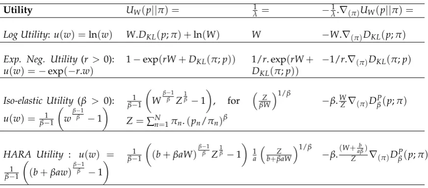
for connections of HARA utilities to divergences and scoring rules by Jose et al.

[2008]. The HARA utility u(m) = _β−1₁

(b+βam)

β−1

β −1

(for a > 0) is defined on the domain b+βam ≥ 0 with strict inequality for β ≤ 1. HARA is a general

class of utilities that include the popular quadratic (when β = −1),linear (β → ∞), square-root (β = 2) , log(β → 1),reciprocal (β = 1/2), iso-elastic(power) (β > 0 and

b=0) andexponential negative decay(β→0) utilities. βis considered as arisk-tolerance parameter of the utility1 [Jose et al., 2008; Chen and Pennock, 2007]. The iso-elastic utility (u(m) = _β−1₁

mβ

−1

β −1

) is also calledConstant Relative Risk Aversion (CRRA)

utility since it’s risk aversion is βm, so the risk aversion relative to the wealth is β

(constant). The exponential negative decay utility (u(m) =−exp(−r.m)forr >0) is also called Constant Absolute Risk Aversion (CARA) utility since its risk aversion isr, which is constant with respect to wealth.

Note that the parameters I have adopted for HARA here and in later chapters is compatible with the notation used in Jose et al. [2008] who consider a special case of HARA called Linear Risk Tolerance (LRT) utility by using a=1 and b=1. To avoid confusion with other work that concern prediction markets, I note the following other parametrisations. Chen and Pennock [2007] use a parameterγ(which is a

risk-averseness parameter2_{) which translates to the current setting as}_γ₌ 1

β. Storkey et al.

[2012] use a parameter η for iso-elastic utilities that is compatible with η = γ = _β1.

Wolfers and Zitzewitz [2006] and Hu and Storkey [2014] use a different parametrisa-tion withγthat translates to the current setting as ₁_−γ1 = β.

2.1.4.2 Risk Neutral traders

Risk neutral traders (as opposed to risk averse traders) are also a common assump-tion in predicassump-tion markets. Risk neutral traders arise from HARA utilities when

β → ∞ or η = γ = 0, resulting in Linear utility u(m) = b+am, which are called

risk neutral since their utility for a guaranteed $1₂(x+y)is always the same for their expected utility3for a fair coin toss resulting in $xor $y. Also note that the Risk Pre-mium for risk neutral traders is zero, meaning that the expected wealth of holding a bundlesis always equal to the Certainty Equivalent of the bundle s.

1_{where risk tolerance} _Γ₍_m₎ _{is defined as the reciprocal of the Arrow-Pratt risk-aversion measure}

(−∂2u(m)/∂u(m)), so Γ(m) = (b+βam)/a for HARA utilities, so the risk aversion is a hyperbolic

function of wealth (hence the name Hyperbolic Absolute Risk Aversion).

2_{The risk-aversion measure for HARA utilities is} ₋

∂2u(m)/∂u(m) = a/(b+βam) = a/(b+

(am)/γ), so risk aversion increases asγincreases.

3_{note that their risk tolerance measure is infinite (}_Γ₍_m_{) =}_lim

β→∞(b+βam)/a) =∞, meaning zero

(28)

The assumption of risk neutral traders is a key assumption in Market Scoring Rules designed by Hanson [2007], where it is assumed that risk neutral traders move the market prices to their own beliefs (see Section 2.3.2). This typically assumes that the traders are not restricted by wealth when trading. Risk neutral traders are also used in prediction markets with wealth restrictions (see [Manski, 2006; Storkey, 2011; Othman and Sandholm, 2010]).

2.1.4.3 Convex Risk Based Traders

Even though the MEU framework is widely used, there has also been arguments regarding the rationality of a trader adopting the utility maximising (MEU) concept. For example, Yaari [1987] points out that it may be desirable to separate the notions ofrisk aversionanddiminishing marginal utility of wealthfrom each other, where it be-comes synonymous under expected utility theory.

Also behaviour patterns which are inconsistent with expected utility theory have been observed in practice. For e.g., even thoughFullKelly Betting is viewed as con-sistent with utility theory (for traders maximising log utility),Fractional Kelly Betting

is commonly used in practice, where only a part of a trader’s wealth is used to pur-chase contracts mainly to avoid the high volatility of Kelly betting and to safeguard against inaccurate beliefs. Beygelzimer et al. [2012] view Fractional Kelly Betting as equivalent to Full Kelly Betting with revised beliefs (considering the market prices) with a Bayesian justification4.

Convex risk measure based traders is an alternative trader model to MEU. Formally, a convex risk measure [Föllmer and Schied, 2004] satisfies convexity, monotonicity and translation invariance (discussed in Section 4.2) and has a form

ρ(x) = sup q∈∆N

{hq,−xi −α(q)}

whereα(q)is a penalty function defined on the domainq∈∆N. See Hu and Storkey

[2014] for use of convex risk measure based traders in prediction markets, where traders make demands to minimise their risk measure. In Section 4.2, I give a more detailed discussion of convex risk based traders and it’s relation to potential-based demands.

4_{it would be interesting to find out whether fractional Kelly betting is connected to the convex risk}

(29)

§2.2 Equilibrium prediction markets 18

Convex risk measures have also been derived using the utility framework (see Föllmer and Schied [2004]). One notable special case is the exponential negative decay utility,

u(m) = −exp(−r.m). The negative of its Certainty Equivalent for MEU demands is the well-studiedentropic risk measure

ρ(x) = sup q∈∆N

{hq,−xi − 1

rDKL(q;p)}

where r > 0 and DKL(p;q) = ∑nN=1pn. ln(pn/qn) is the KL divergence. This can

be obtained by solving for MEU demands d(Πq) = x, with trader beliefs p and prices π =q, which results inxn = 1_rln(pn/qn) +W+ 1_r.DKL(q;p)(when the trader

spends his total wealth i.e., hq,xi = W), and then calculating the CE of X which gives CE(X) = (u)−1₍_E

n∼p[u(xn)]) = −[hq,−xi − 1_rDKL(q;p)]. For now assume

π = q = arg sup_q∈_∆

N{hq,−xi − 1

rDKL(q;p)}. Applying exponential negative decay

utility to our Collorary 1 given in Chapter 4, we get that π = qis indeed the

max-imising argument as assumed here.

So we can view traders with exponential negative decay utility as belonging to both MEU and risk-based trader models (since minimising -CE is equivalent to maximis-ing MEU). Thus it becomes interestmaximis-ing to verify whether the results obtained usmaximis-ing exponential negative decay utility based traders using the MEU model (as in Aber-nethy et al. [2014]) could be extended to prediction markets using risk based traders.

2 .

2 Equilibrium prediction markets

For a prediction market in which traders buy and sell Arrow-Debreu contracts, and when traders make demands to maximise their expected utilities, we say that the pre-diction market is in (Walrasian) equilibrium when supply equals demand [Wolfers and Zitzewitz, 2006]. The price for which supply equals demands is called the equi-librium price. So the market equiequi-librium is defined in terms of both the equiequi-librium price and demands of the traders in response to equilibrium prices.

(30)

§2.2 Equilibrium prediction markets 19

d1, . . . ,dK, and for a market with N outcomes trading in Arrow-Debreu contracts representing each outcome, the equilibrium priceπ∗ satisfies,

∀n∈[N],

K

∑

k=1

dk_n(π∗) = K

∑

k=1

hπ∗,dk(π∗)i

A more detailed discussion of equilibrium is deferred to Section 3.1.1.

Market equilibrium is also the classical market analysis technique used in economics. Consider a market which sells a particular “good”. Typically it is assumed that the constant interaction of buyers and sellers enable a price to emerge over time, so that supply equals demand and thus there is no surplus or shortage of goods, thus effi-cient. This single price which brings demand and supply into balance, is called the equilibrium price or market clearing price. Note that this equilibrium price changes if there is a change in supply or demand. However, the market prices prior to emer-gence may be far off from the equilibrium prices, which may also be the case in prediction markets. Understanding this difference is one of the main motivations of this dissertation.

Even though most empirical analysis of prediction markets treat prices of binary outcome contracts as predictions of the probability of future events, this was recently challenged by Manski [2006] who showed that the equilibrium prices resulting from linear utility maximising (or risk neutral) traders does not correspond with the mean beliefs of the traders (he in fact showed that the equilibrium price corresponds with a particular quantile of the budget-weighted distribution of traders beliefs). This was initially answered by Wolfers and Zitzewitz [2006] incorporating risk-averse traders as opposed to risk neutral traders. They show that in a binary outcome prediction market, if the traders are MEU traders with log utility and the same initial wealth, the equilibrium price coincides with the average belief of the traders (similar to the ran-dom forest aggregation), and that if the wealth is correlated with the beliefs, then the equilibrium prediction market price is equal to the wealth-weighted average beliefs (similar to boosting aggregation).

2.2.1 Equilibrium market connections to Machine Learning

(31)

ag-§2.2 Equilibrium prediction markets 20

gregations from machine learning. Using MEU traders, they extend the results of Wolfers and Zitzewitz [2006] to multiple outcome markets, showing that,

• the equilibrium price with log utility based MEU traders result in the

wealth-weighted-mean belief aggregation

• linear utilities result in wealth-weighted-medians,

• exponential negative decay utilities result in product-model combinations such

as log opinion pools or geometric means and

• iso-elastic utilities result in (implicitly weighted) entropic means orα-mixtures.

Also note that in the convex optimisation literature, these aggregations (except the weighted-median) relate to minimisations of divergence-based distances [Ben-Tal et al., 1989; Amari, 2007]. For example if there are [K] participants with beliefs

pk ∈∆_N and weightswk ∈R+_,

• The aggregation π ∈ ∆N that would minimise ∑Kk=1wk.DKL(pk;π) is the w

-weighted-mean belief5, i.e.,πn=∑K_k=1wk.pkn. Storkey [2011] shows that weights wcorrespond to the traders’ wealthsW in the case of log utility based traders. • Similarly, arg min_π∈_∆_N∑K_k=1wk.DKL(π;pk)is the geometric mean,

i.e., πn = c.{exp(∑Kk=1wk. ln(pkn))}(∑ K

k=1wk) where c is a normalization

con-stant. When the traders have exponential negative decay utilities (u(m) = −exp(−r.m)), the weights wcorrespond with 1_r of each trader. Storkey [2011] considers the case where traders are homogeneous, (i.e., all having the same identical utilityu(m) =−exp(−m)withr =1 for all traders).

• And arg min_π∈_∆

N∑ K

k=1wk.DβP(p k_;

π)is thew-weighted entropic mean,6

i.e., πn = {∑Kk=1wk.(pkn)β}(1/β) (also called an α-mixture, for α = 1−2β).

Storkey et al. [2012] show that when traders have iso-elastic utility

u(m) = _β−1₁

mβ

−1

β −1

, each weightwkcorresponds with an implicit weight given by W_Zkk, where Zk =∑nN=1πn. pkn/πn

β

andWk is the wealth of traderk. Further Storkey et al. [2012] show that prediction markets can produce novel ag-gregations by allowing traders with inhomogeneous (different) utilities. By using iso-elastic traders with different parameters of β (or α), they note that the resulting

5_where_D

KL(p;π) =∑N_n₌₁pn. ln(pn/πn)is the KL divergence

6_where_DP

β(p;π) =

∑N

n=1πn.(pn/πn)β−1

β(β−1) forβ>0 are the power divergences, which correspond with

anα-divergenceDα(p;π) =4/(1−α2){1−∑Nn=1(pn/πn)

1−α

(32)

§2.3 Sequential Market Making 21

equilibrium extends theα-mixtures formalism.

Lay and Barbu [2010, 2011] also use artificial prediction markets to obtain the weighted-mean aggregation and implement kernel methods, logistic regressions from traders who use betting functions.

Beygelzimer et al. [2012] show that binary outcome prediction markets with Kelly betters (log utility based traders) redistribute trader wealths according to Bayesian law once the outcome of the market is known, which Storkey et al. [2012] generalize to the class of iso-elastic utility based traders (see Section 2.5).

Even though equilibrium prediction markets have nice connections to machine learn-ing as discussed above, calculatlearn-ing the equilibrium price is always not straightfor-ward (e.g., as shown by Storkey et al. [2012] the equilibrium price of an iso-elastic market is implicitly dependent on itself, requiring an iterative algorithm to calcu-late the equilibrium price). See Vazirani [2007] for a brief summary of processes to solve for market equilibrium including convex optimisation approaches and auction processes. There is work in Economics and Finance which develop on the idea of tatonnement (see Cole and Fleischer [2007], Fleischer et al. [2008]) to compute equi-librium prices. Work from Physics include Tseng et al. [2010] which examine the statistical properties of market agent models.

Equilibrium markets typically use some kind of off-equilibrium trading process that eventually converges to a point (i.e., equilibrium) whose properties are studied. Computational viewpoints to equilibrium computation match to dynamic processes, which could be constructed as a choice of market dynamic, and hence are relevant to this thesis. This thesis provides such a process, taking care to identify the un-derlying behavioral model. The algorithmic and equilibrium analyses are therefore complementary to each other.

2 .

3 Sequential Market Making

(33)

connec-§2.3 Sequential Market Making 22

tions with machine learning. It has been shown by Chen and Pennock [2007] that these are equivalent to cost-function based sequential market makers (described in Section 2.3.3) which is the focus of the rest of this thesis. In Section 2.3.4, I briefly mention some important results that connect cost-function based markets with ma-chine learning. For completeness I mention some other types of sequential markets with market makers (in Section 2.3.5).

2.3.1 The need for a market maker

Most popular prediction markets such as the Iowa Electronic market operate as a continuous double auction. In continuous double auctions which are commonly found in modern stock markets, the buyers submit bids (buy orders) and sellers sub-mit asks (sell orders) for a certain quantity and a trade takes place whenever the two sides match and any outstanding quantities are maintained in an order book, where the incoming orders typically have price/time priority. One problem in information markets of this form is the thin marketproblem. Even though there might be an ex-ponential number of contracts available to trade, traders might only be interested in trading on a certain limited set of contracts of which they are knowledgeable about. Since placing an order (bet) will reveal their personal beliefs, orders that wait a long time to be accepted might be at a potential disadvantage. For these reasons, for a trade to occur, traders must coordinate on the contracts they must trade and when they must trade. So even if one participant possesses some information about a par-ticular event (contract), if no one else is interested, that information will be wasted because the participant will not be able to announce his beliefs [Hanson, 2003].

(34)

[image:34.595.122.521.136.303.2]

Figure 2.1: Screen-shot of an Intrade’s market (from [Pennock, 2010])

The introduction of an automated market maker who is always willing to buy and sell every outcome at some price aims to remove these problems by allowing traders to trade any contract at any time. Even though the market maker stands to bear some loss, it is thought to be well compensated since the motive is to make predic-tions rather than to profit [Hanson, 2003; Pennock, 2010]. In many existing markets, all trades are done with one or more few central market makers and have been adopted in information markets (for e.g., the use of automated market makers in the Hollywood Stock Exchange) [Hanson, 2007].

2.3.2 Market Scoring Rules (MSR)

The sequential market mechanism called Market Scoring Rules (MSR) introduced by Hanson [2003] is based on an automated market maker who uses scoring rules and solves the above problems inherent in sequential markets, thus encourages trading. Here I give a brief overview of MSR markets and the use of scoring rules to elicit trader beliefs.

Scoring rules are a measure of the quality of probabilistic predictions. Suppose a forecaster assigns probabilities to multiple outcomes N and gives a report vector

r ∈ RN_{. A scoring rule defines the payout}_s

n(r), if the nth outcome occurred. Use

of a proper scoring rule (which maximizes the expected score for well calibrated probability assessments) as the payoff function will incentivise the forecaster to re-port his true private beliefs (p). For example if the scoring rule sn(r) determines

(35)

the expected payoff only by reporting his true belief (p) in the report (assuming risk neutral traders i.e., traders with linear utility). Some examples of proper scoring rules for reported vectorr ∈ RN _{and outcome probability vector} _p _∈ _RN _{are given}

in Table 2.1. For unnormalizedr(i.e. ∑_nN=1rn 6=1), the scoring rules can be extended

for a normalized r by using ri/∑nN=1rn for ri [Hanson, 2007]. See Jose et al. [2008]

[image:35.595.113.558.269.454.2]

and Chen and Pennock [2007] for more examples including weighted power and pseudo-spherical scores (also given in Appendix A ).

Table 2.1: Proper Scoring Rule Examples [Hanson, 2007]

Scoring Rule Payoff for outcomen∈[N] Notes

Logarithmic sn(r) =an+b. log(rn) Special case of power law rule

when α= 1 and only

depen-dent on the probability report for outcome n

Quadratic sn(r) =an+2brn−b.hr,ri Special case of power law rule

whenα=2

Brier sn(r) =1−(ρn−rn)2 The original Brier score

[Brier, 1950] which can be derived from the quadratic scoring rule

Power Law sn(r) =an+b.α.R₀rn p_nα−2dρn−b∑nN=1rαn Proper whenα≥1

Spherical sn(r) =an+b.rn/(hr,ri)1/2

Scoring rules do not suffer from the irrational participation and thin market prob-lems, but they have the problem of being unable to produce a single consensus when different people give differing estimates, known as thethick market problem. [Hanson, 2003]

Market Scoring Rules (MSR) are in essence sequentially shared scoring rules that ad-dress the thick market problem. It is used by an automated market maker where a trader can change the current published report (prices) of the market, and be paid according to the new report, as long as he agrees to pay the last trader ac-cording to his report. For any proper scoring rule sn(r), if the trader changed the

published distribution from p to r, he should accept a (net) payment of the form

∆sn(r,p) = sn(r)−sn(p) for outcome n. When there is only one trader, the market

(36)

The most popular example of MSR markets is the LMSR (Logarithmic Market Scor-ing Rule) which uses the Logarithmic scorScor-ing rule (sn(r) = an+b. log(rn)). LMSR is

used by a number of companies including Inkling Markets, Consensus Point, Yahoo! and Microsoft.

Thus the market scoring rules provide incentives for truthful revelation and the se-quential nature of the use of the scoring rule also solves the irrational participation problem seen in prediction markets because traders can always adjust the published report and be paid according to a proper scoring rule. The introduction of an au-tomated maker also solves the thin market problem, because traders can trade with the market maker at any time, so the need to match trades is eliminated. This over-comes the problems of prediction markets and allows to incorporate the information of even a solitary trader [Chen and Pennock, 2007]. It also solves the thick market (information aggregation) problem of scoring rules since the traders share the scor-ing rule. Thus it has the combined advantages of scorscor-ing rules and the information aggregation characteristic of prediction markets [Hanson, 2003].

In traditional markets, market makers are human decision makers seeking to earn a profit (while also providing more liquidity), but in a prediction market the role of the market maker is to elicit information from the traders (by providing incentives), pro-vide liquidity (encourage and facilitate trading) and price discovery (aggregation), so he is expected to lose some money in the process [Chen and Pennock, 2007].

If the market maker published his initial beliefs r0, and there were T subsequent updates before the outcome was revealed to ben, the total loss for the market maker would be∑T_t=1(sn(rt)−sn(rt−1) =sn(rT)−sn(r0). The market maker incurs the

max-imum loss when the final probability estimate (rT) assigns probability 1 to the true outcome, thus the market maker has bounded worst case loss. So in the case of a Logarithmic Market Scoring Rule (LMSR) using sn(r) = an+b. log(rn), the

maxi-mum expected loss for the market maker would be the entropy, −b∑N_n=1r0nlog(r0n)

of the initial distributionr0, withbrepresenting the liquidity of the market [Hanson, 2007]. If the market maker started by publishing a uniform distribution (asr0), then his worst case loss is bounded by b. log(N) in the case of a logarithmic scoring rule and by (N−_N1)b for a quadratic scoring rule (for N discrete outcomes) [Chen and Pen-nock, 2007].

(37)

a prediction market framework with an automated market maker who determines fair prices for the contracts for an infinitesimal amount of trade and who will accept any finite fair bet that is an integral of such infinitesimal trades. Here the traders are asked to give their opinion (in the form of a report r) and the change of contracts required to change the current report is decided accordingly.

2.3.3 Cost-function based sequential markets (CSM)

Chen and Pennock [2007] have showed that Hanson’s LMSR is equivalent to an au-tomated market maker implementing a cost function C(x) = b. log(_∑_nN₌₁exp(xn/b)

for the current amount of contracts sold (x) andb>0 in a prediction market setting. Here the traders express interest in trading some particular amounts of contracts, instead of directly reporting their beliefs. Incost function based sequential markets (CSM) using a convex, differentiable function C : RN → R, a trader has to pay an amount C(xt+1)−C(xt) if he updated the current contract position of the market (total contracts sold so far) to xt+1 _from _xt _{(by purchasing} _xt+1₋_xt _∈ _RN _amount

of contracts). The price of a bundle of contracts depend on the change of contract position in the market, and the cost function C keeps track of the total amount of money the traders have spent so far. The value of ∇C(x)can be seen as the price for buying an infinitesimally small bundle at position x and is therefore called the

instantaneousprice at x (denoted byπ). For e.g., the LMSR has instantaneous prices πi = _∑Nexp(xi/b)

n=1exp(xn/b).

Chen and Pennock [2007] show equivalent relations and how to translate between CSM and MSR markets and also between another type of market (namely Constant Utility based Market Makers briefly mentioned in Section 2.3.5). Agrawal et al. [2011] further analyse this and give conditions for which these relations hold.

Formally, CSM markets use asequential pricing mechanism Π(·|s1, . . . ,sT)∈ P which is a function from histories of bundle purchasess1_{, . . . ,}_sT _{for any number of trades} T to pricing functions. Specifically,

ΠC,x0₍_s_|_s1_{, . . . ,}_st_{) =}_C₍_xt₊_s₎₋_C₍_xt₎_{, where}_xt₌ _x0₊

∑

t i=1

si. (2.1)

(38)

histories s1, . . . ,st. Theorem 1 of Abernethy et al. [2011] show that all path indepen-dent sequential pricing mechanisms are necessarily the cost function-based pricing functions (briefly mentioned in Section 2.1.3.1).

If the cost function defines instantaneous prices ∇C(x) ∈ ∆_N for all x, this ensures that the prices set by a cost function are probabilities and cannot be arbitraged (i.e., if the prices summed to something less than (respectively, greater than) 1, then a trader could buy (respectively, sell) small equal quantities of each security for a guaranteed profit) [Chen and Vaughan, 2010]. Also see the related discussion in Section 3.3.3. Chen and Vaughan [2010] note that convex cost functions which defines instanta-neous prices in theN-simplex can be represented in a similar form to the convex risk measures (briefly introduced in Section 2.1.4.3)

C(x) = sup

π∈∆N

{hπ,xi −α(π)} (2.2)

where α:∆N → (∞,∞]is a convex, lower semi continuous function referred to as a penalty functionand arg sup_π∈_∆_N{hπ,xi −α(π)}is the instantaneous prices∇C(x)of

the market.

Abernethy et al. [2011] define generalised cost functions using a duality based rep-resentation (see Section 3.2.1) where the instantaneous prices are not restricted to be in the N-simplex by defining contracts with arbitrary payoff functions (in addition to the standard Arrow-Debreu contracts). They show that the range of the instanta-neous prices is the domain of the dual function. We adopt this duality based cost function representation for the rest of the thesis, particularly in Chapter 3, where we relate sequential price updates with the dual representation of price updates in stochastic mirror descent (see Section 3.2.2).

2.3.4 CSM connections to Machine Learning

Sequential cost function based markets have many connections with the learning-from-expert-advice setup. First they are known to have the property of bounded loss for the market maker, which is similar to regret analysis in online learning algorithms. The worst-case loss of the maker depends on the maximum payment that the market maker may have to pay to the traders, i.e., maxn∈1,...,N{(xTn−x0n)−

∑T

t=1(C(xt)−C(xt−1))} = maxn∈1,...,N{(xTn −x0n)−(C(xT)−C(x0))}, if the market

was initialised with the initial contract position x0 and the market ended with the final position xT _after _T _{rounds of trading. So}₍_xT

Prediction Markets for Machine Learning: Equilibrium Behaviour through Sequential Markets