Singular value computations on the AP1000 array computer

(1)

APlOOO ARRAY COMPUTER

A THESIS

SUBMITTED FOR THE DEGREE OF MASTER OF SCIENCE OF THE AUSTRALIAN NATIONAL UNIVERSITY

By Adam Czezowski

(2)

(3)

1,

•

I hereby declare that this submission is my own work and that, to the best of my knowledge and belief, it contains no material previously published or written by another person nor material which to a substantial extent has been accepted for the award of any other degree or diploma of a university or other institute of higher learning, except where due acknowledgement is made in the text of the thesis.

f;U

~

(/ Adam Czezowski

lll

(4)

(5)

The topic of the thesis presented herein is computations of singular value decomposition on the APlOOO array computer. This topic is part of the joint ANU-Fujitsu research project on 'Linear Algebra Research on the APlOOO'.

This research was undertaken as part-time study at the Computer Science Department of the Australian National University from April 1991 to April 1995. The supervision for this work was provided by Dr Peter Strazdins; and Professor Richard Brent acted as an advisor.

Aim of this research work

The primary drive to pursuit this research was the possibility of working on the experimen-tal, at the time, pa allel computer APlOOO from Fujitsu. Thanks to Dr Peter Strazdins who proposed the subject of this research, this interest gained essence and provided me with the opportunity to learn about numerical linear algebra.

The main aim of this research is to provide thorough investigations of porting a singular value decomposition algorithm from a single to a multi-processor environment. We would like to present the key factors which help to make such a move in the best possible manner. We wish to accomplish this task by analysing the performance of the SVD algorithm on each level of the parallel memory hierarchy. We also will address all those issues which may contribute to the degradation of performance of the algorithm at a particular level of memory hierarchy.

The key issues which we will try to resolve are choice of the algorithm to implement, suitability of the APlOOO architecture for the implementation of the chosen algorithm, reduction of the floating point operations, best match between the implementation and the network topology, communication, cache performance, and register usage.

(6)

Ii

Publications arising from this study

Progress of this research was presented at the joint AND-Fujitsu Workshops and the

Parallel Computing Workshops held in Japan, on an annual basis (91-94) and published

in the respective proceedings [9, 3, 11]. The preliminary results were also presented at the

5th Australian Transputer and OCCAM User Group Conference TAPA-92, in Melbourne,

in November 1992, and were published in the conference proceedings [10].

The final results of this thesis were delivered in a poster session at the International

Conference and Exhibition on High-Performance Computing and Networking HPCN-1994,

held in Munich, April 1994 and were included in the conference proceedings [8].

Also due course of this research two seminars were delivered at the Computer Science

Department of the Australian National University.

Reading guide

Chapter 1 presents the theory of singular value decomposition with its rich historical

back-ground, various SVD serial algorithms, and some scientific and engineering applications

of the SVD.

Chapter 2 discusses choices of the suitable algorithm and architecture, introduces the

APlOOO architecture, and presents the basic block implementation of the Hestenes SVD

algorithm on the APlOOO.

Chapter 3 introduces the improvements of the floating point performance by

reduc-ing the number of floatreduc-ing point operations. This chapter also addresses the issues of

measurement and comparison of the performance of different versions of the algorithm

implemented.

Chapter 4 demonstrates the optimisations on all levels of parallel memory hierarchy:

other processors' memory (communication), cache and register levels. It introduces the

reuse factors as a general measure of the performance on all parallel memory hierarchy

levels.

Chapter 5 addresses the issues of convergence and the accuracy of various

implemen-tations of the SVD algorithm.

Chapter 6 draws conclusions from this research and proposes new research paths on

the subject of SVD which emerged during this work.

(7)

Firstly, I am very grateful and wish to thank most of all Dr Peter Strazdins for his excellent supervision in the course of my study, especially for his high degree of professionalism, teaching quality, and his understanding of a part-time student. Also I would like to acknowledge his contribution to the most of the material presented in Chapter 3 and 4 of this thesis. I also appreciate and wish to thank my advisor Professor Richard Brent for the 'light in the darkness of errors propagation' and his support throughout the course of my research.

I especially thank Professor Steve Redman from the Department of Neurophysiology of the John Curtin School of Medical Research for his encouragement to undertake this study.

I am also very grateful to my wife, Loan, for her love, support and patience shown during this degree.

Finally, I am much obliged to the Department of Computer Science for the generous financial assistance which enabled me to present the results of my research overseas and to the departmental staff, programmers and system administrators, for keeping both kaffa and APlOOO alive most of the time.

(8)

(9)

....

The increasing popularity of singular value decomposition algorithms, used as a tool in

many areas of science and engineering, demands a rapid development of their fast and

reliable implementations. No longer are those implementations bounded to the single

processor environment since more and more parallel computers are available on the

mar-ket. This situation requires that often software need to be re-implemented on those new

parallel architectures efficiently.

In this thesis we show, on the example of a singular value decomposition algorithm,

how this task of changing the working environments can be accomplished with non-trivial

gains in performance. We show several optimisation techniques and their impact on

the algorithm performance on all parallel memory hierarchy levels (register, cache, main

memory and external processor memory levels). The central principle in all of the

opti-misations presented herein is to increase the number of columns (column-segments) being

held in each level of the memory hierarchy and therefore increase the data reuse factors. In

the optimisations for the parallel memory hierarchy the techniques used are, rectangular

processor configuration, partitioning, and four-column rotation.

The rectangular processor configuration technique is where the data were mapped onto

a rectangular network of processors instead of a linear one. This technique improves the

communication and cache performance such that on average, we reduced the execution

time by a factor of 2 and, in the case of long column-segments, by a factor of 5.

The partitioning technique involves rearranging data and the order of computations

in the cells. This technique increases the cache hit ratio for large matrices. For the

relatively modest improvements in the cache performance of 2 to 5%, we achieved a

significant reduction in the execution times of 10 to 20%.

The four-column rotation technique improves the performance by a better register

reuse. For the cases of large number of columns stored per processor, this technique gave

(10)

optimisations are presented on the algorithm itself which can be applied in any

archi-tecture. The main ideas behind those optimisations are the reduction of the number of

floating point instructions executed in a unit of time and the balance of the floating point

operations. This was accomplished by reshaping the relevant parts of the code to use the

APlOOO processors architecture (SPARC) to its full potential.

After combining all of the optimisations, we achieved a sustained 60% reduction of

the execution time which corresponds to the 2.5 fold reduction. In the cases where long

columns of the input matrix were used, we achieved nearly 5 fold reduction in execution

time without adversely affecting the accuracy of the singular values and maintaining the

quadratic convergence of the algorithm.

The algorithm was implemented on the Fujitsu's APlOOO Array Multiprocessor, but

all optimisations described can be easily applied to any MIMD architecture with a mesh

or hypercube topology, and all but one can be applied to register-cache uniprocessors also.

Despite many changes in the structure of the algorithm we found that the convergence

was not adversely affected and the accuracy of the orthogonalisation was no worse than

for the uniprocessor implementation of the noted SVD algorithm.

(11)

u

Statement

Preface

Acknowledgements

Abstract

1 Introduction

1.1 Singular value decomposition - theoretical approach 1.1.1 Orthogonality . . .

1.1.2 Vector and matrix norms 1.1.3 SVD theorem . . . 1.2 Historical background of the SVD .

1.2.1 The roots of the SVD . 1.2.2 Bilinear form and SVD 1.2.3 Integral form and SVD .

1.3 Uniprocessor algorithms for SVD computations 1.3.1 Jacobi methods . .

1.3.2 1.3.3 1.3.4

Hestenes algorithm QR based algorithm

Implicit zero-shift QR based algorithm . 1.4 Scientific and engineering applications of the SVD

(12)

2 Parallel Implementation of the SVD 33

2.1 Introduction . 33

2.2 General approaches to the linear algebra parallel, high performance

com-puting 34

2.3 Which algorithm? . 35

2.4 Which architecture? 37

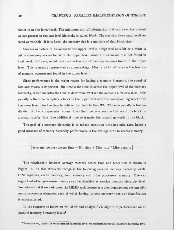
2.5 Parallel memory hierarchy 39

2.6 APlOOO architecture 41

-

2.6.1 APlOOO - hardware environment 41

-

2.6.2 APlOOO - software environment 45

2.6.3 APlOOO - performance 46

2.7 Hestenes algorithm implementation 48

2.7.1 Systolic array implementation 49

2.7.2 Block implementation 53

2.8 Conclusions 55

3 Improvements of the Floating Point Performance 57

3.2 Measuring and comparing performance . 58

3.3 Scaled columns 61

3.3.1 Numerical results . 62

3.4 Reduced inner product computations 65

3.5 Assembly language optimisations 67

3.5.1 Rotation procedures 67

3.5.2 Inner product computation procedures 68

3.6 Conclusions 70

-

4 Optimisations for the Memory Hierarchy 73

4.1.1 General performance measures - reuse factors 74

4.1.2 Measuring and comparing performance . 74

(13)

4.2 _{Optimisations on other processors memory level .}

75 4.2.1 Rectangular cells configuration

75 4.2.2 Numerical results

77

4.3 Optimisations on cache level .

80 4.3.1 Partitioning

80 4.3.2 Numerical results

82

4.4 Optimisations on register level ₈₄

4.4.1 Four-column rotation ₈₄

4.4.2 Register reuse . ₈₆

4.4.3 Effect on the convergence ₈₆

4.4.4 Numerical results ₈₇

4.5 Conclusions

89

5 Convergence

93

5.1 General error propagation issues ₉₃

5.2 General convergence rate issues ₉₆

5.3 Numerical results ₉₇

5.3.1 Initial data distribution ₉₇

5.3.2 Accuracy of the methods implemented ₁₀₁

5.4 Numerical results for convergence rate ₁₀₂

5.5 Conclusions ₁₀₂

6 Conclusions ₁₀₅

xiii

(14)

(15)

'

List of Tables

2.1 Completion times for global functions (in

µs).

. .

. . . .

. .

.

. .

47 3.1 Results for the basic, unimproved Hestenes algorithm implementation. 60 3.2 Results for the scaled implementation of the Hestenes algorithm. . . 63 3.3 Results for the a-update implementation of the Hestenes algorithm. 67 3.4 Scaled columns implementation after assembly language modifications. 69 3.5 The reduced inner product implementation after assembly language

modi-fications. . . . . . . . . . . . . . . . . . . . . . . . . . . . . . . 71 3.6 Comparison of efficiencies for the original and improved algorithms. ₇₂ 4.1 Relative performance improvements for the rectangular configuration. 78 4.2 Communication times in X and Y directions for the rectangular configuration. 78 4.3 The best results for the rectangular configuration. . . . . . 79 4.4 Cache performance comparison for the partitioning method. 82 4.5 The best results for the rectangular configuration with partitioning. 83 4.6 Register reuse in Q2 and Q4 schemes . . . . . . . . . . 86 4.7 The best results for the four-column implementation without partitioning. 87 4.8 The best results for the four-column implementation with partitioning. . 88 4.9 The overall best results for Hestenes SVD algorithm implementation. . . 90 5.1 Floating point parameters for the IEEE compliant computer and APlOOO. 94 5.2 Test results for the basic block implementation. . 98 5.3 Test results for the rectangular implementation. . 99 5.4 Test results for the four-column implementation. 100 5.5 Off(A)/N after each sweep for the rectangular implementation. 101 5.6 Off(A)/N after each sweep for the four-column implementation. 102

(16)

(17)

1.1 Single processor, Hestenes algorithm implementation . . . . 1.2 Selected singular value outer product images of Mandrill Baboon .. 1.3 Selected partial sums of the SVD of Mandrill Baboon images. 1.4 Linear SVD edge sharpening of Mandrill Baboon image. . . 1.5 Nonlinear SVD edge sharpening of Mandrill Baboon image. 1.6 Frequent letters in the Gettysburg Address. . . . . 2.1 The average memory access time as a function of block size. 2.2 APlOOO - photograph. . . . . .

2.3 APlOOO - system configuration.

2.4 APlOOO - cell configuration . . . 2.5 APlOOO - pingpong performance. 2.6 Binary tree and y ...sum performance. 2.7 Example of inter-processor connections.

2.8 Systolic array data flow for SVD algorithm.

2.9 Communication in systolic array implementation.

2.10 Execution time for the systolic implementation. 2.11 Data flow in block implementation . . . .

2.12 Execution time for the block implementation. 2.13 Efficiency for systolic and block implementation. 2.14 Execution time for the single processor run . . . .

14

24 26 27

28

31

41

42

43

44

47

48

49

50

51 52

53

54

55

4.1

Distribution of columns for rectangular cells configuration. .

76

4.2 Main loop for the rectangular configuration and the partitioning method. 81

(18)

II

Introduction

The word algebra, in its original Arabic form (al dzabr, al gabr), was used for the first time by Muhammed ibn Musa al Chwarizmi in the ninth century (30]. This word was used to describe the operation of transposition of the unknowns from one side of the equation to the other.

Until the end of the nineteenth century, algebra was primarily used for solving equa-tions. Later on, it developed and transformed into a fully mature, axiomatic science. This modern and 'new' algebra chooses as a subject, abstract rules performed on sets of any nature. Soon after, new algebraic ideas and concepts, thanks to their universality, became an indispensable tool for the whole of mathematics as well as theoretical physics, theoretical chemistry and other scientific disciplines.

Today, most of the pre-nineteenth century algebra is known as linear algebra and among its many topics, it deals with general linear systems, matrix analysis, orthogonali-sation, eigenvalue problem and last, but certainly not lea.st, singular value decomposition.

Although theoretical linear algebra is well developed, its practical, numerical approach still has a lot of room for improvement. We all want that algorithms of linear algebra will be faster and more accurate, portable and scalable. New parallel computer architec-tures leave us with the challenge of porting efficiently existing linear algebra software and developing new one.

In this thesis we show how rich and fruitful can be the task of moving a linear algebra algorithm from single processor environment to multiprocessor one. We present the key factors which help to realize such a move in the best possible manner.

(19)

ii

mathematical beauty and numerous applications. Another reason, a very practical one,

was to evaluate the suitability of Fujitsu's APlOOO Array Processor for numerical algebra

applications. Since most previous work on the linear algebra on the APlOOO [5] involved

non-iterative computations, the SVD was a natural choice to be implemented as the

iterative algorithm.

In this chapter we describe the subject of singular value decomposition, its very

in-teresting historical background, various uniprocessor SVD algorithms and finally, some

examples of SVD applications.

1.1 Singular value decomposition - theoretical approach

First, we would like to establish some definitions which will be widely used throughout this

thesis. We introduce definitions of: vector orthogonality, norms, matrix rank, orthogonal

transformations, eigenvalues and eigenvectors. We pattern our definitions after Golub's

and Van Loan's book 'Matrix Computation' [21].

1.1.1 Orthogonality

Orthogonality is a key factor in SVD computations, therefore we will define this term

firstly.

Definition 1.1 Two vectors Xi and

x;

in

mm

are orthogonal if

xf x;

=

O whenever i =/= j. Definition 1.2 Two vectors Xi and

x;

in

mm

are orthonormal if

xf x;

=

Oij where Oij is the Kronecker symbol.

Definition 1.3 Let X

= {xi, ... , xp}

be a set of vectors in

mm

.

We say that vectors in

X are orthogonal if all the pairs of vectors in X are orthogonal.

Definition 1.4 Let X

={xi,

...

, xp}

be a set of vectors in

mm.

We say that vectors in

X are orthonormal if all the pairs of vectors in X are orthonormal.

For example in the Euclidean space the set of the unity vectors parallel to the axis of the

Carthesian coordinate system is orthonormal.

Definition 1.5 A matrix A E

mmxm

is orthogonal if AT A= I where I is identity matrix.

In other words, the column-vectors of A,

[iii, ... , iiml,

are orthogonal.

Very often orthonormal matrices are called unitary.

(20)

I

1,

1.1. SINGULAR VALUE DECOMPOSITION - THEORETICAL APPROACH ₃

1.1.2 Vector and matrix norms

The norms are the class of the functions which introduce measure into the vector spaces. A function f which projects element x of the vector space V into field

n

can be called a norm on

V

if

f

satisfies the following properties:

f(x)?:_O and f(x)=O<=}x=O

f(ax)

=

lalf(x)

where a

En

f(x

+

y)

:S

f(x)

+

f(y)

Definition 1.6 A vector norm

llxll

on IRn belongs to the class of the p-norms if

(1.1)

(1.2)

The vector norm that is mostly used in this thesis is

llill2

=

(lx112

+· ·

·+lxnl2

)t

=

(x7'x)t.

Similarly we define two most frequently used matrix norms.

Definition 1. 7 A matrix norm

IIAJJ

on mmxn belongs to the class of the p-norms if

def

II

Ail

Ip

IIAII

=

IIAIIP

= sup

II-II

where p

?:

1.

x/0 X p (1.3)

If p

=

2 the above norm is called 2-norm or Euclidean norm.

Definition 1.8 A matrix norm

IIAII

on mmxn can be called the Frobenius norm if m n

IIAII

~f

IIAIIF

=,

t1

~

laiil

2•

(1.4)

There is a very important class of transformations called orthogonal transformations. The main property of these transformations is that they preserve 2-norm and the ma-trix Frobenius norm. An example of the orthogonal transformation in JR2 _{is rotation}

matrix Q2:

(

cos </> sin </> )

Q2= .

- sin </> cos </>

(1.5)

1.1.3 SVD theorem

(21)

4 CHAPTER 1. INTRODUCTION

Theorem 1.1.1 (SVD) For rmy real m-by-n matrix A there are orthogonal matrices

U

= [u1, ...

1 Um] and V

=[vi, ...

1 Vn] such that

UTAV=diag(cr11 • • • ,crp) where p=min{m,n} and cr1zcr2z···crnzO.

The CTi are called singular values1 of A and the vectors Ui and

Vi

are the ith left and ith right singular vector respectively.

Let us define the concepts of subspace, range, null space and rank which are associated with an m-by-n matrix A.

Definition 1.9 The set of all linear combinations of the vectors

v1, ... ,

Vn E mn is called

subspace and referred to as the span{ v'1, ... , v'n}.

Definition 1.10 The range of matrix A, range(A), we call set of vectors y E mm such that for some X E mn y

=

Ax.

Definition 1.11 The null space of matrix A, null(A), we call set of vectors x E mn such

that Ax= 0.

Definition 1.12 The rank of the matrix A, rank(A), is the maximal number of its

inde-pendent rows or columns.

Having these definitions we can show how well SVD can describe properties of a given matrix A. If the singular values of the matrix A are

cr1z ...

CTr

>

CTr+l

= ... =

CTp

=

0 where p

=

min{m, n} then

rank(A)

=

r

null(A)

=

span{vr+i, ... ,vn}

(1.6)

range(A)

=

span{u1, ... , ur}

Moreover, the 2-norm and the Frobenius norm can be nicely expressed in terms of the SVD:

IIAIIJ;.

=

crf

+ ... +

cr;

(1.7)

1

In the past also known as the principal values.

h

I

.,

(22)

1.2 Historical background of the SVD

There are two reasons why we dedicate this section to the history of the SVD. Firstly, we would like to show that the development of the SVD was a long process and many people, to whom we would like to pay tribute, contributed a lot to it. Secondly, we believe it is much more appropriate to study SVD being aware of its background, as it is said that the frame gives a picture dignity.

The beginning of many of new ideas in mathematics have often their multiple sources and if so, it is usually difficult, if not impossible, to clearly establish the people behind their discoveries. Although the early history of SVD is not that blurred, there are more than five people who can be credited for its creation and development. It is really up to us how we interpret the historical facts and in this thesis we are convinced by and follow the research of G. W. Stewart [42].

1.2.1 The roots of the SVD

In his paper [42], G. W. Stewart starts the history of SVD by giving an intriguing ob-servation that most of the classical matrix decompositions were known before widespread use of matrices. The latter were expressed in form of determinants, linear systems of equations, and especially bilinear and quadratic forms. There is no doubt that the K. F. Gauss is the founder of this area.

In 1829 A.L. Cauchy described the properties of eigenvalues and eigenvectors of a symmetric system. Seventeen years later C.G. Jacobi [28] published his famous2 _algorithm for diagonalising a symmetric matrix and later, after his death in 1851, his paper on LU decomposition was published.

In 1868 K. Weierstrass, in his 'Theory of the bilinear and quadratic Forms', came up with the canonical forms for pairs of bilinear functions which today should be identified as the generalized eigenvalue problem.

Now, we are ready to describe two different ways of introducing SVD: the first through the bilinear form which is the continuation of the line presented above and the second through the integral form which is the domain of integral equations, developed in the first decade of our century.

2

(23)

1.2.2 Bilinear form and SVD

Three names can be mentioned if we talk about an algebraic way of introducing SVD.

There are Eugenio Beltrami (1835-1899), Camille Jordan (1838-1921) and James Joseph

Sylvester (1814-1897). According to G.W. Stewart, Beltrami was the first to introduce

SVD into algebra by publishing his concept in 'Giornale di Matematiche ad Uso degli

Studenti Delle Universita' in 1873. The purpose of his paper was to introduce bilinear

forms to the students of Italian universities. Beltrami makes substitutions for

i

=

U[

and

iJ

=

Vij (matrices U and V are required to be orthogonal) in the following bilinear form

( matrix A is real and of order n)

f(x,

Y)

=

xT

AiJ, (1.8) so that after

f (

x,

iJ)

=

f'

Sij, (1.9)

where

S= UTAV. (1.10)

If we assume that Sis diagonal (S

=

E

=

diag(a1 , . . . , an)) then by using the fact

that matrix U and V are orthogonal we can establish the following relations:

UT A

=

EVT and AV

=

UE. (1.11)

After multiplying the first relation of Equations 1.11 by AT from the right hand side and

the second relation from the left hand side Beltrami obtains the following equations:

(1.12)

From the above we can see that Cli are the roots of the following characteristic polynomials:

det(AAT - a2 I)= 0 and det(AT A - a2 I)= 0. (1.13)

In order to show that singular values ai are distinct and nonzero Beltrami argues that the

last two equations are identical because they are polynomials of degree n that have the

same values at a= Cli and the common value det2(A) at a= 0. Moreover, using the fact that O

<

ii# AiJF

=

#(AAT)i, Beltrami shows that the

a'f

are positive.

At the end of his paper, Beltrami gives the recipe for diagonalising matrix A: (1) find

roots of the det(AAT - a2_I)

=

_{0, (2) determine}_U_{from the}_UT(AAT)

=

_E2_UT_{and (3)}

get V from the uT A

=

EVT.

'

(24)

11

1.2. HISTORICAL BACKGROUND OF THE SVD

7

This is the sketch of Betrami's path which led him to the singular value decomposition for a real, square, nonsingular matrix having distinct singular values.

In Stewart's paper, Camille Jordan is given the status of a co-discoverer of the singular value decomposition. From his paper published a year after Beltrami, we clearly see that the work is independent.

In his paper, Jordan seeks the maximum and minimum of the form represented by

P=xAy

_(1.14)

subject to

IJxllF

=

IIY11F

=

1. The maximum is determined by the equation

(1.15) which must be satisfied for all

dx

and

dy

that satisfy

(1.16)

According to Stewart, the following argument of Jordan is not quite clear and he proposes that for some constants u and T we must have

(1.17) Since

dx

and

dy

are independent we can write two equations:

A -_y

₌

_{ux an}- d _x-TA

₌

_Ty-T _. _(1.18)

From the first of the above equations, we see that the maximum is

(1.19) and from the second, the maximum is

( -TA)~ x Y;

=

TY -T-y

=

T, (1.20)

so that u

=

T. Now, Jordan states that a is determined by the vanishing of the

determi-nant

D= -al A

AT -al

Then he shows that this determinant contains only even powers of a.

(1.21)

(25)

I

Let a₁be a root of the equation D

=

0, and let i

=

u

and

y

=

v

be the solution of

the 1.18 equations, where

lliZIIF

=

llvllF

=

1. Also, let

U

=

(iZU)

and

V

=

(vV) (1.22)

be orthogonal, and let

i

=

(Jf and

y

=

v§.

(1.23)

Following these substitutions, Jordan lets

-T ...

-P

=

x

Ay. (1.24)

After substitutions, P attains its maximum and at the maximum we have

... - - -T A -T

Ay

=

a1x and x A= a1y , (1.25) which implies that

(1.26)

Thus with

6

=

f

1 and 7/1 =

ff

1, P assumes the form

(1.27)

where P1 is independent of

6

and 7/1· After applying reduction to

Pi,

Jordan comes to

the canonical form

(1.28)

Jordan's approach of using a partial solution of the problem is to reduce it to the

smaller size. By doing so, he avoids the degeneracies that complicate Beltrami's approach.

Joseph James Sylvester wrote two papers and a footnote on the subject of the singular

value decomposition. All three were published in 1889. The footnote of his paper, in

which he describes an iterative algorithm for reducing a quadratic form to diagonal form,

contains suggestion that the analogous iteration can be used to diagonalise a bilinear form.

Sylvester's algorithm described in his later paper resembles Beltrami's one.

1.2.3 Integral form and SVD

During the first two decades of our century the topic of integral equations played a

sig-nificant role in mathematics. In 1907, Erhard Schmidt, well known from Gram-Schmidt

(26)

I:

orthogonalisation method, introduced the infinite dimensional analogue of SVD and for-mulated his approximation theorem. He showed that if two functions g and h are contin-uous and

A(s, t)

is continuous and unsymmetric kernel on

[a,

b]

x

[a,

b]

then

l

blb

1

lb

b

a a

A(s, t)g(s)h(t)dsdt =~Ai

a

g(s)u

i(

s

)

ds

1 h(t)vi(t)dt,

t

(1.29) where

u(s) =Alb A(s, t)v(t)dt

and

v(t) =Alb A(s, t)u(s)ds

_(1.30) is a pair of adjoint eigenfunctions corresponding to the eigenvalue A. Schmidt says the above expression 'corresponds to the canonical decomposition of a bilinear form'.

In his second contribution, the approximation theorem, Schmidt solves the problem of finding the best approximation to matrix A of the form

k

A~

Lxtif[

_(1.31)

i=l

in the sense that

k

I/A -

L

X

i

Yfll

=min. (1.32)

i=l

He starts by pointing out that if

(1.33) then

k

IIA - AkllF

=

IIAIIF

-

Lu;.

(1.34)

i=l

Schmidt shows that if for an arbitrary

X

i

and

Yi

the below inequality is fulfilled

k k

IIA -

L

X

i

WII

~

IIAIIF -

Lu;,

(1.35)

i=l i=l

then

Ak

is the desired approximation.

An important application of the approximation theorem is the determination of the rank of a matrix in the presence of an error. If A is of rank k and

A

= A + E, then the last n - k singular values of

A

satisfy

(1.36) so that the defect in rank of A will be manifested in the size of its trailing singular values.The above inequality is actually a perturbation theorem for the zero singular values of a matrix.

(27)

..

-Herman Weyl's contribution to the theory of the SVD was to develop a general per-turbation theory and use it to give an elegant proof of Schmidt's approximation theorem.

In 1913 Autonne extended the decomposition to complex matrices. Eckart (1936) and

Young (1939) extended it to rectangular matrices and rediscovered Schmidt's approxima-tion theorem.

According to G. W. Stewart, the term 'singular value' most likely came from the literature on integral equations. It appeared first in Schmidt's paper but in our modern meaning, it was used in 1937 in the publication by Smithes.

1.3 Uniprocessor algorithms for SVD computations

There are two main stream methods for computing the singular values. The first one is based on plane rotations (Jacobi rotations)3 [28] and was introduced by Kobetliantz [29] in 1955 and developed further by Hestenes [26], Forsythe and Henrici [15]. The second one is based on the QR algorithm and was suggested by Kublanovskaya [31] in 1961. The computational algorithm based on the QR method was introduced into numerical analysis by Golub and Kahan [19] in 1965. In 1970 Golub and Reinsch [20] published the Algol SVD procedure which has been the basis for the Eispack 2 and Linpack SVD

subroutines. In 1990, Demmel and Kahan [12] proposed an interesting alternative to the SVD algorithm.

1.3.1 Jacobi methods

Firstly we would like to present Jacobi diagonalising scheme as it is the core of all non QR-based SVD algorithms. The basic principle behind Jacobi methods is to perform a sequence of orthogonal updates At- QT AQ after which, each new matrix A is "closer" to the diagonal than its predecessor. These methods are iterative and usually there is some convergence criteria associated with them.

In 1846, Jacobi described his idea of reducing a matrix to the diagonal form [28]4 •

He achieves that by systematic reduction of the quantity

n n

of f(A)

=

LLafj

(1.37)

~ i=l j=l

j-::/:.i

3

Jacobi rotations are no different from Givens rotations (21]. 4

Jacobi's original paper is one of the earliest references found in the numerical analysis literature (21] .

(28)

ii

To reduce of f(A) he applies rotations of the form 1

0

J(p, q, e)

=

0

cos(e)

- sin(8)

0 p

0

sin(e)

cos(e)

0

q

0

0 p

0 q

1

(1.38)

Jacobi procedure requires choosing index pair

(p

,

q)

such that 1::;

p

<

q:::;

n , computing e such that

[

bpp bpq

l [

cos(8) sin(8)

l

T [ aPP apq

l [

cos(8) sin(8)

l

bqp bqq

=

sin(e) cos(e) aqp aqq sin(e) cos(e) (1.39) is diagonal, and overwriting A with B

=

JT AJ where J

=

J(p, q, 8). Since the Frobenius norm is preserved by Jacobi transformation, we can write

of f(B)2

=

of f(A)2 - 2a~. _(1.40) The above equation shows what it means that A moves closer to diagonal with each Jacobi step.

The sin(8) and cos(8) are computed according to the following 2-by-2 symmetric Schur decomposition. To diagonalise 1.39 is to set

0

=

bpq

=

apq(cos2(8) - sin2(8))

+

(app - aqq) cos(e) sin(8). (1.41) If apq =

0

then we set (sin(8), cos(8)) =

(0

,

1)

. Otherwise we define

a -a

(

=

qq PP and t

=

sin(8)/ cos(e)

2apq (1.42)

and

t

=

tan(8) solves the following quadratic equation

t2

+

2(t - 1

=

0. (1.43)

The two roots of the above equation are represented by sign(()

(29)

Ii

The sin(0) and cos(0) can be computed from the formulae

cos(e) =

~

andsin(e) = tcos(e). 1

+

t2

(1.45)

Choosing the smaller of the two roots of the equation 1.44 ensures that 101 ~ 7r /4 and

minimises the difference between B and A in the Frobenius norm sense.

The above introductory consideration leads us to the classical Jacobi algorithm which

overwrites a given, symmetric, n-by-n matrix A with matrix D = VT AV where V is

orthogonal and of f(D) ~ €

II

A

IIF·

The c is a tolerance and c

>

0. In this classical Jacobi

algorithm, to maximise the reduction of the quantity of f(A), we choose the pair

(p, q)

so

that

a~

is maximal. Since

lapq

l

is the largest off-diagonal entry, it follows that

(1.46)

where N = n(n -1)/2 (see note below)5 represents all possible choices of pairs

(p, q)

such that p

=/-

q. From equation 1.39 we get

off(b)

2 ~ (1-

~

)k

off(A)

2.

(1.47)

By induction, after k Jacobi updates, we obtain

(1.48)

which means that the classical Jacobi procedure converges at a linear rate. However,

Schonhage (1964) and van Kempen (1966) [21] showed that the asymptotic convergence

of the above algorithm is quadratic.

The original Jacobi method is inefficient in choosing the optimal pair

(p, q).

This

searching process involves O(n2₎_{operations while the Jacobi updates involve only}_O(n)

operations. To solve this problem we can step cyclically through all the pairs in

row-by-row fashion. This is called cyclic-by-row-by-row Jacobi algorithm. For example, if n=5 we cycle

as follows:

(p, q)

= (1, 2), (1, 3), (1, 4), (1, 5), (2, 3), (2, 4), (2, 5), (3, 4), (3, 5), ( 4, 5), (1, 2), ... (1.49)

The cyclic-by-row Jacobi algorithm also converges quadratically and is considerably faster

than Jacobi's original algorithm. Another type of Jacobi algorithm is the threshold Jacobi,

6

It is customary to refer to N Jacobi updates as a sweep(21].

I•

(30)

[,

:

II

where we skip the annihilation of apq if its modulus is less than some small,

sweep-dependent parameter. We can use Jacobi diagonalisation method to solve the symmetric eigenvalue problem which can in principle be used to solve the SVD problem. For example, we may compute the eigenvalue decomposition

VT (AT A)V

=

diag(af, ... , a~),

where V

=

[v1,

... ,

vn] is orthogonal and O"i satisfies

0-1

2 · · ·

2

O"r

>

O"r+l

= ·

·

· =

O"n

=

0, with r

=

rank(A). We next calculate the vectors

Avi

U i = -

(i=l, ...

,r),

O"i

(1.50)

(1.51)

(1.52) and then determine the vectors Ur+l, ... , Um so that the matrix U

=

[u1,

... ,

um] is orthogonal. The factorisation UT AV= diag(o-1, ... , an) gives the SVD of A. The above shows that theoretically we can compute an SVD of A by an eigenvalue decomposition of AT A. Practically this is not a good idea because the explicit formation of AT A can lead to well-known numerical difficulty of ill-conditioning if matrix A is nearly dependent. This

problem was addressed and solved by Hestenes who applied the Jacobi method implicitly.

1.3.2 Hestenes algorithm

In 1958 Magnus Hestenes published in his paper the method for obtaining singular values via applying Jacobi rotations on one side6 _{SVD of the matrix}_A._{The Hestenes algorithm} proceeds as follows.

We want to generate an orthogonal matrix V such that the transformed matrix AV= W has orthogonal columns. Having the matrix W, we normalise the length of each non-null column to unity i.e.

W(:,i)

O"i

=

I

w(

:,i)

I,

u( :,i)

= ----;,;-

and

w

=

UE . (1.53) That is the way we obtain the matrices U and E. An SVD of the matrix A is given by:

AV= W-rAV = UE-rA = UEVT. (1.54)

6

(31)

flag=l

for k=l:50

\*

Beginning of the kth sweep

*\

if flag=l

for i=O:n-1 for j=i+l:n

flag=O

(k) _ A(k) A(k)

O'.ii ·. - ( :,i ") ( :,i ")

(k) _ A(k) A(k)

a ₃₃.. - ( _:,₃.) ( _:,3.)

(k) _ A(k) A(k)

O'._t3·. - ( _:,t") ( _:,3") (le)

if aii ~ € a\~l+a(~)

n JJ

flag=l

(le) (le)

c(k) - ajj -aii

<:, - (le)

2a ..

'3

t(k) - sign(e(le))

- 1e<1e>1+.J1+e<1ei2

cos e(k) = l j sin e(k) = t(k) cos e(k)

-/1+t<1ei2

A (k-:f"I) = rotate (A (k) A (k)_ sin e(k) cos e(k))

(:,t) (:,i)' (:,3)' '

A(k~I) = rotate (A(k~ A(k)_ sine(k) cose(k))

(:,3) (:,i)' (:,3)' '

v;(k.+I)

= rotate (V:(k) v:(k~ sin e(k) cos e(k))

(:,t) (:,i)' (:,3)' '

V,(k_+I) = rotate (V,(k) V,(k~ sin 9(k) COS 9(k))

{:,i) (:,i)' (:,3)' '

end 1f end for end for end if end for

function: A(r+l) = rotate (A(r) A(r) sine(r) cose(r))

(:,p) (:,p)' (:,q)' ' X = A(r) cose(r) - A(r) sin e(r)

( :,p) ( :,q)

y = A(r) sin e(r) + A(r) cose(r)

(:,p) (:,q)

A(r+l)

=

X (:,p)

A(r+l) -₍_:_,) _{- y}

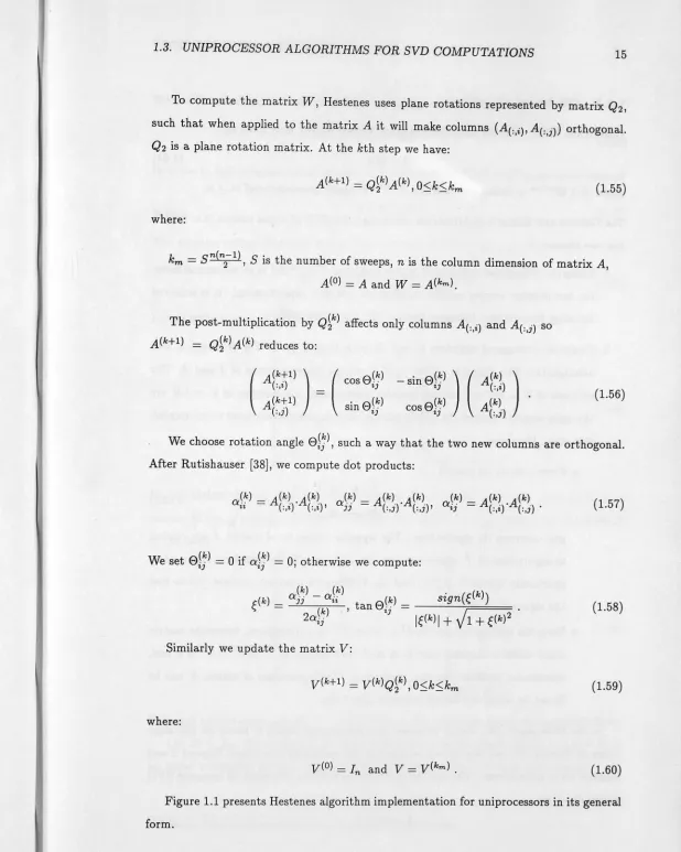
[image:31.646.9.615.15.798.2]

en;I rotate

Figure 1.1: Single processor, Hestenes algorithm implementation.

I

(32)

i

I

To compute the matrix W, Hestenes uses plane rotations represented by matrix Q

2,

such that when applied to the matrix A it will make columns (A(:,i), A(:,j)) orthogonal.

Q2 is a plane rotation matrix. At the kth step we have:

(1.55)

where:

km= 3n(n_2- 1), Sis the number of sweeps, n is the column dimension of matrix A,

A(o) = A and W = A(k.n).

The post-multiplication by Q~k) affects only columns A(:,i) and A(:,j) so

A(k+l)

=

Q~k) A(k) reduces to:

(

A (k~l) ) ₍_:_,i) _- ( cos e(~) - sine(~) ) ( _tJ _tJ A (k~ ) ₍_:,i₎

A (k~l) - sine(~) cos e(~) A (k)_

(:,J) tJ tJ (:,J)

(1.56)

We choose rotation angle efj), such a way that the two new columns are orthogonal.

After Rutishauser [38], we compute dot products:

(1.57)

We set e(~) _tJ

=

0 if a/~) _tJ

=

O·, otherwise we compute:

(1.58)

Similarly we update the matrix V:

(1.59)

where:

[image:32.632.3.621.22.795.2]

v(o)

=

In and V

=

v(k.n) . _(1.60)

Figure 1.1 presents Hestenes algorithm implementation for uniprocessors in its general

(33)

II

-

.

1.3.3 QR based algorithm

Definition 1.3.1 The QR factorisation of an m-by-n matrix A is given by

A=QR (1.61)

where Q E IRmxm is orthogonal and RE IRmxn is upper triangular and m 2'.: n.

The Golub's and Kahan's algorithm for computing the SVD of a real matrix A= UEVT

has two phases:

1. Compute orthogonal matrices P and L such that J

=

pT AL is in bidiagonal form,

i.e. has nonzero entries only on its diagonal and first superdiagonal. It is achieved

by using Householder bidiagonalisation [21, pages 236-238].

2. Compute orthogonal matrices G and H such that E

=

GT J H is diagonal and

nonnegative. The diagonal entries ai of E are the singular values of J and A. The

columns of U = PG are the left singular vectors, and the columns of V = LH are

the right singular vectors. In [19] Golub and Kahan give two methods to accomplish

this step. They are:

• Form a 2n-by-2n matrix

(1.62)

and compute its eigenvalues. The singular values ai of matrix J are related

to eigenvalues of

i,

which are just +ai and -ai. To do that form tridiagonal,

symmetric matrix T

=

f(J)

and use Wilkinson's bisection method [45] to find

the eigenvalues of T.

• Form the tridiagonal matrix JT J. Since JT J is a tridiagonal, hermitian matrix

there exists a diagonal matrix b. such that matrix K

=

b.(JT J)b.T is a real,

symmetric, positive and also tridiagonal. The eigenvalues of matrix K can be

found by using the Sturm sequence algorithm.

In his 1968 paper [18], Golub proposed another method which is based on QR

algo-rithm of Francis (16] and was widely adopted in the previously mentioned Eispack 2 and

Linpack SVD subroutines. The method proceeds as follows. We want to compute SVD

of matrix A, so

(34)

I

We use Householder bidiagonalisation to compute matrix J such that

J

=

pT AL. _(1.64)

In order to find singular values of matrix J, we construct SVD of J in the usual form of

(1.65) The singular values of matrix A and J are the same7. Thus, we can write

EJ

=

ar J H

=

ar pr A LH

=

E .

'--v--' '-v-' (1.66)

UT V

Let us write matrix J explicitly.

I I

a1 /31 0 0

0 _{a2 /32} 0

0 0 0 _f3n-1 (1.67)

0 0 0 an

0 }(m-

n)

X

n.

\ )

In [19] Golub showed that the eigenvalues of the following symmetric and tridiagonal matrix K are

±

singular values of J. So the task now is to find eigenvalues of matrix K

of the form

I \

0

(1.68)

0

2n X 2n.

This task can be accomplished by using Francis's QR algorithm which proceeds as follows. Let K

=

K0• We compute the factorisation Ko

=

QoRo where Q'{; Qo

=

I and Ro is

an upper triangular matrix. After multiplying the matrices in reverse order we get

(1.69)

7

(35)

Now if we treat K1 ,in the sam~ way as the matrix Ko we will obtain sequence of matrices

defined as follows:

(1.70)

We can accelerate the convergence of the QR method by choosing right shift parameter

s(i):

(1.71)

Since the eigenvalues of K always occur in pairs, we will compute the QR decompo

-sition of

(1.72)

so that

Q(i) R(i)

=

K2 (i) _ S2 (i) J . _(1.73)

In his paper [16], Francis showed that it is not necessary to compute (1.73) explicitly but

it is possible to perform the shift implicitly. Let N(i)(:, 1)

=

Q(i)(:, 1) and NT (i)N(~)

=

I.

Then the Francis theorem states that if

ii)

T(i+l) is a tridiagonal,

iii) K(i) is non-singular,

iv) the subdiagonal elements of T(i+l) are positive,

it follows that T(i+l)

=

K(i+l). Now diagonalise matrix K using the quite simple approach

(36)

'

!

I

It

•

Let us define matrix z~i)

(p) (p

+

1)

(p

+

2)

I

1

0 1

cos ()p 0 sin ()P

_(p)

z(i)

=

p 0 1 0

_(p+

1) (1.74)

sin ()P 0 -cos ()p

_{(p+ 2)}

1 0

1 _{2n x}_2n.

The cos 81 is chosen so that

zI

i) ( K2 ( iJ - s2 ( iJ

I) (:,

1)

=

o .

_(1.75)

Due to the Francis theorem we have

K (i+i) -_- T(i+iJ -_- z(i) _{2n-2 · · ·}z(i)Kz(i) ₁ _{1 ·}_·_·z(i) _{2n-2 ·} _(1.76)

The product of all the orthogonal transformations gives the singular values and yields the matrix of orthogonal eigenvectors of K.

The Golub and Reinsch [20] variation differs from the above algorithm only in the way matrix K is transformed to the diagonal. The transformation 1.76 in the Golub and Reinsch algorithm looks as follows:

K (i+lJ

=

sT (iJsT n n-1 (il · · · 5T 2 (ilJr.(ilr.(iJ 2 3 • · · n r(.:J , (1.77)

where the matrices T(i) are chosen so that the sequence JT (i)J(i) converges to a diagonal matrix while the matrices s(i) are chosen so that all J(i) are of the bidiagonal form. So, both algorithms differ only in the technique of deriving 5(i) and T(i).

Let us summarize this standard algorithm. We apply Francis QR algorithm implicitly

to JT J. The algorithm computes a sequence of J,: of bidiagonal matrices starting from

(37)

1,

I

!

eigenvalue of the bottom 2-by-2 block of J; Ji, Then the algorithm does an implicit QR factorisation of the shifted matrix J; Ji - s2 I= QR where Q is orthogonal and R upper triangular, from which it computes a bidiagonal Ji+l such

/f+

1 Ji+l

=

RQ

+

s2 I. With i,

Ji converges to a diagonal matrix with the singular values on the diagonal.

In (21, page 239] we can find that Golub-Reinsch algorithm requires 4mn2 - 4n3 /3 flops if only singular values of A are desired and 4m2n

+

8mn2

+

9n3 if whole SVD of

matrix A is needed.

1.3.4 Implicit zero-shift QR based algorithm

In the 'standard' (Golub-Reinsch) algorithm, the error of the computed singular values CTi

of matrix A is no bigger that p(n) ·E· IIAll2 ((21, pages 246-248]), where IIAII

=

cr1, € is the

machine precision, and p(n) is a slowly growing function of the dimension n of A. This means that the singular values of order of IIAll2 are computed to high relative accuracy. However, small singular values can not be generally computed with high relative accuracy. Demmel and Kahan in their paper (12] proposed an algorithm which can compute the singular values for bidiagonal matrices to the same relative precision as the individual matrix entries. Using paraphrase, if all the matrix entries are known to high relative accuracy, all the singular values can be computed to high relative accuracy independent of their magnitudes. Let us define the relative perturbation of value a.

Definition

1.3.2 We say 8a is a relative perturbation of a of size at most 1J if l8al

s;

7Jlal.

If A is a matrix then IAI and l8AI denote the matrices of absolute entries of A and 8A. The following is the central theorem, upon which Demmel's and Kahan's algorithm is based.

Theorem [12, page 875] 1.3.1 Let J be an n-by-n symmetric tridiagonal matrix with

zero diagonal and off-diagonal entries b_{1 , . . . ,}bn-l· Suppose J +8J is identical to J except

for one off-diagonal entry, which changes to abi from bi, a=/- 0. Let

a=

max(lal, la-11),

Let Ai be the eigenvalues of J sorted into decreasing order, and let

>.~

be the eigenvalues

of J

+

8J similarly sorted. Then

>.

.

I

~<>.

_a

_{_}

i

-

<

_

a>.

i

· .

(1.78)

(38)

•

1.3. UNIPROCESSOR ALGORITHMS FOR SVD COMPUTATIONS ₂₁

The proof of the above theorem is given in [12, page 876].

Next, Demmel and Kahan use the fact that the eigenvalues of

J

of the form

(1.79)

are the± singular values of J and some zeros. (See Section 1.3.3). From the last theorem 1.3.1 and the above fact they obtained following corollary.

Corollary [12, page 877] 1.3.1 Let J be an n-by-n bidiagonal matrix and suppose <>]ii+ Jii = a2i-1Jii, <>Ji,i+l

+

Ji,i+l = a2Ji,i+1, O'.j -=p 0. Let

a

=

rrt1

1 max(IO'.il, lai1

J).

Let u1

2:: ... 2::

Un be the singular values of J, and let u~ 2:'. ...

2::

u~ be the singular values of

J

+

JJ. Then

(1.80)

Thus, if for example l-71:::; lail:::; 1+71, then no singular value can change by more than

a factor of

a

= (1 - 71)1-2n. The above corollary may be contrasted with the following classical perturbation bound for singular values of Wielandt-Hoffman.

Theorem [21, page 429] 1.3.2 Let u1

2::

...

2::

Un be the singular values of A, and let

u~

2::

..

.

2::

u: be the singular ~alues of A+ JA. Then

Ju; - uil:::; ll<>AJJ.

The Demmel's and Kahan's algorithm corresponds to the 'standard' when the shifts= 0

and therefore is called zero-shift QR algorithm. Their final algorithm is a hybrid of the 'standard' QR and implicit zero-shift QR. Standard QR is used when the condition number of matrix J, which is defined as the ratio of the largest to the smallest singular values, is small. The roundoff errors make small perturbations in the smallest singular values of J which, in this case, can be accepted. If the condition number is large, the implicit zero-shift QR is used instead.

The most inner loop of the zero-shift QR algorithm has only four multiplications beside two calls to ROT (rotation) procedures. This is in contrast to the standard algorithm which in addition to two calls to ROT has twelve multiplications and four additions. Also, Demmel's and Kahan's algorithm is more parallelizable than 'standard' one. 8

Apart from computing singular values to full machine precision, this alternative algo-rithm is generally faster than the 'standard' one, and ranges from 2.7 times faster to 1.6

(39)

I

times slower counting reduction to bidiagonal form (7.7 times faster to 3.4 times slower

not counting reduction to bidiagonal form).

1.4 Scientific and engineering applications of the SVD

The singular value decomposition not only is important as an algebraic concept which

serves linear algebra on its own but also has numerous applications in science and

engi-neering. In recent years, the SVD has become a fundamental tool for the formulation of

new concepts in signal processing such as angles between subspaces, oriented

signal-to-signal ratio, canonical correlation analysis and for the reliable computation of the solutions

to problems such as total linear least squares or source separation by subspace methods.

The development of new techniques used for image enhancement and image compression

has been also based on SVD.

1.4.1 Least Squares problems

In the linear algebra, the SVD plays an important role in a number of least squares

problems. Let us give some examples which will illustrate that.

El. Let

Un

be the set of all n x n orthogonal matrices. For an arbitrary n X n real matrix A, determine Q E

Un

such that

IIA - QIIF

:s;

IIA - XIIF

for any X E Un,. (1.81)

The solution for this problem comes from Fan and Hoffman [14]. They showed that if

A=

U:EVT, then Q

=

uvT. (1.82)

E2. An important generalization of the above problem occurs in factor analysis. For

arbitrary n X n real matrices A and B, determine Q E

Un

such that

IIA -

BQIIF

:s;

IIA - BXIIF

for any X E Un,. (1.83)

It has been shown by Green [22] that if

BT

A=

U:EVT, then Q

=

uvT. (1.84)

E3. Let

M~~n

be set of all m X n matrices of rank

k.

Assume

A

E

M~~n

-

Determine

B E

M~~n (k

:s;

r)

such that

(40)

I'

..

In 1936, Eckart and Young [13] showed that if

A= UEVT, then B

=

UO.kVT _(1.86)

where

'

0"1 0 ... 0

0 0"2 ... 0

nk

=

...

. . .

_.

.

_{. . . .}

_(1.87)

0 0

.

..

O"k

0

It is worth to observe that

(1.88)

E4. An n X m matrix X is said to be the pseudo-inverse of an m x n matrix A if X

sat-isfies the following four properties: AXA= A, XAX = X, (AXf = AX, (XAf = XA. We denote the pseudo-inverse by A+. We wish to determine A+ numerically. In [36] Penrose shows that A+ can always be determined and is unique. One can verify that A+ is given by

(1.89)

where

I

'

...1.. ₀

_...

₀ 0-1

0 _!__ _0-₂

..

.

0

A=

. . . . . . ... .

.

(1.90)

0 0

..

.

...1.. _U}c

0 _nxm.

(41)

Figure 1.2: Selected singular value outer product images of Mandrill Baboon. (i) Original (ii)

(i11v'f)

(iii)

(i15vg)

(iv)

(i131vl1)

1.4.2 Image analysis

The example below was taken from a paper of H.C. Andrews and C.L. Patterson published in the IEEE Transactions on Acoustics, Speech, and Signal Processing [2].

Through the development of the theory of linear filtering, SVD has its permanent place in signal processing along with such a fertile tool as FFT. The methods used by Andrews and Patterson are simple extensions of the theory of linear filtering. We already know that any matrix

[G]

can be represented in a space defined by orthonormal matrices

[U]

and

[V]

as

[G]

=

[U][A]1f2[Vf

.

(1.91)

From SVD of matrix

[G]

we have that if

(1.92)

and

[image:41.650.13.627.15.800.2]

(42)

I

where the terms iii and Vi are the column-vectors of

[U]

and

[V],

respectively, then

ifI' ₁

-Y

[G]

=

[ii1ii2, ... , iln][A] 1

l

2 V2 _(1.94)

if1'

n

where

-;.. 1/2

1 0 0 0 0 0 0 0

0 0 0 ,\1 -112

[A]1/2

=

₊

_{+ ....}

_(1.95)

0 0 0 0

From the above, the expansion of the matrix [G] can be represented in the vector outer product notation as

R

[GJ

=

I:

x:12aii!f.

(1.96)

i=l

The upper limit of the sum R is the rank of matrix [G] . If

[G]

is nonsingular, R

=

n. This outer product notation can be viewed as a summation of R matrices of rank one, each weighted by the square root of the respective singular value

-;..f

2• After this introduction Andrews and Patterson merge both SVD and the matrix representation of the image. Any image can be defined as an array of the pixels where each value of the array represents optical intensity of the pixel and is usually a positive number. Let us refer to this matrix as matrix [G]. From SVD, an image represented by [G] may be decomposed into a sum of rank one matrices (images) which can be called eigenimages (ii/if{). Figure 1.2 illustrates the technique on a 128 X 128 image known as the 'Mandrill baboon'. The figure presents, absolute-value versions of the first, sixth, and thirty-first outer product matrices obtained from the decomposition of the original.

The fact that a computer provides the singular values which are not zero but are quite small (i.e. 10-11₎ _{can be used to reduce storage space for the image.}_If_{an approximate}

representation of the matrix [G] is formed by truncation, then K

[GK]=

L

XJ

12 uivT

(1.97)

(43)

(i)

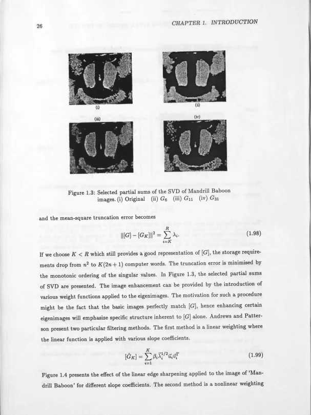
Figure 1.3: Selected partial sums of the SVD of Mandrill Baboon

images. (i) Original

(ii)

G6