Bayesian system identification of dynamical systems using highly informative training data

promoting access to White Rose research papers

White Rose Research Online

[email protected]

Universities of Leeds, Sheffield and York

http://eprints.whiterose.ac.uk/

This is a copy of the final published version of a paper published via gold open access

in Mechanical Systems and Signal Processing.

This open access article is distributed under the terms of the Creative Commons

Attribution Licence (http://creativecommons.org/licenses/by/3.0), which permits

unrestricted use, distribution, and reproduction in any medium, provided the

original work is properly cited.

White Rose Research Online URL for this paper:

http://eprints.whiterose.ac.uk/83948

Published paper

Bayesian system identification of dynamical systems using

highly informative training data

P.L. Green

n

, E.J. Cross, K. Worden

Department of Mechanical Engineering, University of Sheffield, Mappin Street, Sheffield S1 3JD, United Kingdom

a r t i c l e i n f o

Article history:

Received 5 July 2013 Received in revised form 20 May 2014

Accepted 9 October 2014 Available online 4 November 2014

Keywords:

Nonlinear system identification Bayesian inference

Markov chain Monte Carlo Shannon entropy Tamar bridge

a b s t r a c t

This paper is concerned with the Bayesian system identification of structural dynamical systems using experimentally obtained training data. It is motivated by situations where, from a large quantity of training data, one must select a subset to infer probabilistic models. To that end, using concepts from information theory, expressions are derived which allow one to approximate the effect that a set of training data will have on parameter uncertainty as well as the plausibility of candidate model structures. The usefulness of this concept is then demonstrated through the system identification of several dynamical systems using both physics-based and emulator models. The result is a rigorous scientific framework which can be used to select‘highly informative’subsets from large quantities of training data.

&2014 The Authors. Published by Elsevier Ltd. This is an open access article under the CC BY license (http://creativecommons.org/licenses/by/3.0/).

1. Introduction

To be practically useful, any system identification method needs to be able to quantify and propagate the inevitable uncertainties which arise as a result of noise-contaminated measurements, as well as the fact that one's chosen model structure will never be able to perfectly replicate the physics of the system of interest. Consequently, system identification is best approached using probability logic such that, rather than searching for the‘perfect model’, one is able to assess the relative plausibility of a set of models as well as the parameters within those models[1]. As a result of seminal papers in the machine learning[2]and structural dynamics [3]communities, it is now widely accepted that both levels of inference (parameter estimation and model selection) can be achieved using a Bayesian approach.

With regard to parameter estimation, the plausibility of a model parameter vector

θ

¼ f

_θ

1;…;

θ

NDg given a model

structureMand training dataDcan be expressed using Bayes' Theorem:

Pð

θ

jD;MÞ ¼PðDj

θ

;MÞPð

θ

jMÞ

PðDjMÞ : ð1Þ

One's belief in the plausibility of

θ

before the training data were known is represented by the prior distributionPð

_θ

jMÞ, while one's belief in the plausibility of

θ

after the training data are known is represented in the posterior distribution Pð

_θ

jD;MÞ.PðDj

_θ

;MÞis termed the likelihood and represents the plausibility that the training dataDwas witnessed given

Contents lists available atScienceDirect

journal homepage:www.elsevier.com/locate/ymssp

Mechanical Systems and Signal Processing

http://dx.doi.org/10.1016/j.ymssp.2014.10.003

0888-3270/&2014 The Authors. Published by Elsevier Ltd. This is an open access article under the CC BY license (http://creativecommons.org/licenses/by/3.0/).

n_{Corresponding author.}

model structureMand parameter vector

θ

. The evidencePðDjMÞis essentially a normalising constant given by

PðDjMÞ ¼Z ⋯Z PðDj

θ

;MÞPð

θ

jMÞd

θ

1⋯d

θ

ND ð2Þ

thus ensuring that the posterior probability distribution integrates to unity. When dealing with nonlinear systems, the evidence integral is often intractable and, as a result of the curse of dimensionality, cannot practically be evaluated numerically when the number of unknown parameters is greater than 3.

To surmount this issue one can choose to generate samples from the posterior distribution using Markov chain Monte Carlo (MCMC) methods, which can be implemented without having to evaluate Eq.(2). While many MCMC methods have been developed (see Refs. [4–6]for a comprehensive discussion), by far the most popular is the Metropolis–Hastings (MH) algorithm. This involves the evolution of an ergodic Markov chain through the parameter space such that it is able to converge to, and then generate samples from, the posterior distribution. Ensuring that the chain has converged to the globally optimum region of the parameter space (rather than a‘local trap’) is a nontrivial problem which has led to the development of the well-known Simulated Annealing algorithm [7](and its many variants [8–10]) and, more recently, the Adaptive Metropolis–

Hastings[11], Transitional Markov chain Monte Carlo[12]and Asymptotically Independent Markov Sampling[13]algorithms. Once converged, MCMC can then be used to generate samples from the posterior. These samples can be used to analyse parameter correlations, to propagate one's uncertainty in the parameter estimates and to conduct a sensitivity analysis of the model structure of interest (see[14,15]for example). While undoubtedly useful, MCMC tends to be expensive, as many model runs are usually required before one can build up a reasonable ‘picture’ of the posterior distribution. This is compounded by the fact that, by the nature of MCMC, the samples have not been generated independently and are in fact correlated with each another. Consequently, to avoid making biased estimates, it is often the case that many of the samples generated by MCMC need to be‘thrown away’such that the correlation between the remaining samples is reduced (this process is typically referred to asthinning). To alleviate this issue one may choose an alternative to the MH algorithm such as Hybrid Monte Carlo (HMC)[16]which tends to produce samples which are less strongly correlated than the MH algorithm (HMC is discussed in the context of structural dynamics in[17]). However, as HMC utilises estimates of the gradient of the posterior distribution–which incurs additional computational cost–the author's have found that the ability of HMC to outperform the MH algorithm is very dependent on the problem at hand.

To reduce the computational expense of Monte Carlo analysis one may choose to utilise emulators (also known as meta-models or surrogate meta-models) which are inferred directly from the training data rather than from the underlying physics of the system (see[18]for example). The relatively simple structures of emulators often make them considerably easier to analyse, and computationally cheap when compared to physics-based models.

The work in this paper specifically addresses the situation where, to perform Bayesian system identification as part of some collaborative work, one is presented with a very large quantity of data from which to infer probabilistic models. In such a scenario–particularly if one is aiming to utilise physics-based models–it is usually desirable to select a small subset of the training data to reduce the computational cost of running MCMC.1In such a scenario one would ideally select a subset of data which is both short andhighly informativewith regard to one's parameter estimates. Consequently, the first aim of this paper is to provide a framework which allows one to view the information content–specifically with regard to one's parameter estimates–of large sets of training databeforethe application of MCMC. This allows one to select subsets of data which are both small, and from which one can learn a great deal about the parameters of a candidate model.

The second aim of this paper is with regard to the second level of inference: model selection. Whether using physics-based models or emulators, any system identification procedure will involve choosing a modelMfrom a set of candidate model structures (as implied by Eq.(1)). This task is complicated by the fact that model performance cannot be judged simply by how well a model is able to replicate a set of training data as this will lead to overfitted models based on redundant parameter sets. This issue can be addressed by using model selection criteria such as the AIC[20]or the BIC[21], which reward model fidelity while also penalising model complexity. Alternatively, one can phrase the model selection problem using Bayes' Theorem:

PðMij Þ ¼D

PðDjMiÞPðMiÞ

PðDÞ ð3Þ

whereMiis a model from a set of candidate model structuresM¼ fM1;…;MNMg. Assuming that there is no prior bias over

any of the models inM, one can then rate the relative plausibility of two competing model structures (modelsMiandMj

for example) by computing a Bayes Factor:

β

i;j¼

PðMijDÞ

PðMjjDÞ:

ð4Þ

The Bayes Factor is a model selection criterion which, it can be shown, penalises overfitting without the introduction ofad hocpenalty terms (see[1,2,6,22]for more details). Recent work[23]has also shown that such an approach can also be used

1

to aid in the selection of the prediction-error model used in the likelihood, although this is not investigated in the present paper.

With the second level of inference in mind then, building on the aforementioned idea of‘highly informative’training data, the second major aim of the present work, is to identify which sets of training data will be the most informative with regard to model selection. This develops the idea that an informative set of training data will aid the model selection procedure, by demonstrating that one particular model is much more plausible than the other competing structures.

The paper is organised as follows.Section 2addresses parameter estimation specifically. Expressions allowing one to approximate the effect of a set of training data on the posterior covariance matrix are derived inSection 2.1, before being linked with concepts from information theory as well as previous work from the machine learning community[24] in

Sections 2.2and2.3. These concepts are then extended to the case of model selection inSection 3. The various benefits of

using highly informative training data with regard to parameter estimation and model selection are demonstrated using a series of examples inSections 4and5, where the system identification of a synthesised nonlinear system using a physics-based model and of the Tamar bridge using an emulator are investigated.

2. Parameter estimation

2.1. Taylor series expansion

The case where there areNDparameters to be identified (such that

θ

ARND) is considered here. The parameters are to be

inferred using training dataDwhich consists of a vector of inputs and corresponding outputs of the system of interest. It is assumed that each measured data point is corrupted by Gaussian white noise with variance

σ

2_{, such that the likelihood is}

given by

PðD

θ

;M¼ ∏N

n¼1

ð2

_πσ

2_Þ1=2_exp 1

2

σ

2ðznz^nð

θ

ÞÞ 2

ð5Þ

wherezis the measured response of the real system andz^is the response of the model.

It is well known that, by approximating the log-likelihood (Lð

_θ

Þ) using a second-order Taylor series expansion (see[6]for more details) and assuming an uninformative prior, the posterior can be approximated according to

Pnð

θ

jD;MÞ ¼PðDj

θ

^;MÞ PnðDjMÞ exp

1

2½

θ

θ

^A½

θ

θ

^

T

ð6Þ

where

θ

^ is the most-probable parameter vector and, throughout this work, asterisks are used to denote quantities which have been approximated in this manner. The matrixAis the Fisher Information matrix:

Ai;j¼ ∂

Lð

_θ

Þ2

∂

θ

i∂

θ

j

_θ¼θ^ ð7Þ

whose elements can, depending on the problem at hand, be evaluated analytically or approximated using finite difference methods.

Integrating Eq.(6)with respect to

θ

allows one to write the evidence as

PnðD Mj Þ ¼PðDj

_θ

^;MÞ

ffiffiffiffiffiffiffiffiffiffiffiffiffiffi

ð2

_π

ÞND

jAj

s

: ð8Þ

For the sake of clarity, the Gaussian approximation of the posterior will be written as

Pnð

θ

jD;MÞ ¼ 1 Znexp

1

2½

θ

θ

^A½

θ

θ

^

T

ð9Þ

where

Zn¼

ffiffiffiffiffiffiffiffiffiffiffiffiffiffi

ð2

_π

ÞND

jAj

s

: ð10Þ

Although an improper prior distribution has been utilised in this case, it should be noted that the analysis detailed herein will apply to situations where one has employed a uniform prior distribution whose limits are far from the main region of probability mass (it is also relatively easy to extend the arguments presented here to the case where Gaussian priors are used). In fact, such an analysis is not particularly relevant to the concepts presented in this paper because, as it will be shown, the prior distribution has no influence on the informativeness of the training data.

The covariance matrix ofPnð

_θ

jD;MÞis given by

C¼A1

If one assumes that the off-diagonal elements of the covariance matrix are negligible thenA1

will be a diagonal matrix with elements:

Ai;i1¼

∂2_Lð

θ

_Þ

∂

θ

2 i

_θ¼θ^

!1

ð12Þ

(this is equivalent to assuming that any parameter correlations present in the system are negligible). Consequently, by monitoring the diagonal elements of_A:

Ai;i1; i¼1;…;ND ð13Þ

as more data points are added to the training data, it is possible to see the effect that these points have on the confidence one has in each individual parameter estimate–a drop inAi;i1as training data is added indicates that one's confidence in

the parameter

θ

ihas increased. In fact, it was found to be more convenient to monitor

lnðA1

i;i Þ; i¼1;…;ND ð14Þ

as training data is added, simply for visualisation purposes. The relative simplicity of this expression is helped largely by the fact that it has been assumed that the covariance matrix is diagonal. InSections 2.2and2.3of this work it will be shown that this allows one to develop an intuitive interpretation of the Fisher Information matrix as well as an information theoretic interpretation of highly informative training data. However, it is important to recognise that this assumption is not necessary in practice–Eq.(7)can be used to evaluate the‘full’Fisher Information matrix if it is thought to be necessary. Indeed, by doing so, one may be able to monitor the off-diagonal terms of the covariance matrix as training data is added, thus allowing one to assess which parts of the training data will be informative with regard to the parameter correlations. The effect of assuming a diagonal covariance matrix is analysed in more detail through the use of an example inSection 4of this work.

2.2. Interpretation of the Fisher Information matrix

This section is concerned with the development of a more detailed analysis of the Fisher Information matrix (A) such that a more complete definition of what is meant by‘informative’training data can be developed.

If one considers the log-likelihood:

L

θ

¼ N 2ln 2

πσ

2

1

2

σ

2 ∑ N

n¼1

Jn

θ

ð15Þ

(where Jn¼ ðznz^nð

θ

ÞÞ2) then, differentiating twice with respect to the elements in the parameter vector and utilising

Eq.(7), the Fisher Information MatrixAbecomes

A¼ H

2

σ

2 ð16Þ

whereHis a Hessian matrix whose elements are defined as

Hi;j¼ ∑ N

n¼1

∂2_J nð

θ

Þ

∂

θ

i∂

θ

j

_θ¼θ^: ð17Þ

As a result, the covariance matrix ofPnð

θ

jD;MÞis given by

C¼2

σ

2H1

: ð18Þ

As before, it is assumed that the off-diagonal terms are zero such that the covariance matrixCis diagonal with elements given by

Ci;i¼2

σ

2 ∑ N

n¼1

∂2_J nð

θ

Þ

∂

θ

2 i

_θ¼θ^

!1

: ð19Þ

This allows one to define what is meant by the term‘informative’training data. Firstly, Eq.(19)shows that the diagonal elements of the covariance matrix will increase with the measurement noise variance (

σ

2_{). This provides the rather intuitive}

observation that training data will be more informative if one makes low noise measurements (this point was also made in [24]). Secondly, Eq.(19)shows that one can achieve a large decrease in elementCi;iof the covariance matrix through the

introduction of a data point for which∂2_Jð

_θ

_Þ=∂

_θ

2

ij_θ¼_θ^ is large. In other words, a point of training data can be considered

to be informative (with regard to parameter

θ

i) if the ability of the model to replicate that point is very sensitive to changes

2.3. Relation to the Shannon entropy

Intuitively, it seems reasonable to assume that there is a link between the derivation shown in Section 2.1 and information theory. This is because one would say that a data point which has a great effect on one's parameter estimates contains more information than that which has relatively little effect. This concept was investigated as far back as 1992[24] within the context of machine learning, where the ‘informativeness’of training data was analysed using the Shannon entropy as an information measure. While, within the structural dynamics community, it has been shown that the Shannon entropy can be used to optimise sensor placement and/or experimental design (see [25–27] for example), the authors believe that it has not previously been used to analyse the information content–with regard to both levels of Bayesian inference–of large sets of training data.

The main focus of this section is to calculate the Shannon entropy of the posterior such that a relation between the afore mentioned work in[24]and that presented inSection 2.1of the current work can be drawn.

Noting that the Shannon entropy is a measure of uncertainty then, ergo, the aim here is to select a subset of training data which will reduce the Shannon entropy of the posterior as much as possible. It is important at this point to emphasise that this approach is different from that of the Maximum Entropy (MaxEnt) method[28]which, for example, can be used to find the prior distribution which assumes the smallest amount of additional information. In the current paper the term‘highly informative’is not used to describe distributions with large entropy–it is used to refer to data which can greatly reduce the uncertainty in one's parameter estimates and, consequently, the entropy of the posterior distribution.

Using the Gaussian approximation given in Eq.(6), the Shannon entropy of the posterior is given by

S¼ Z Pn

θ

D;MÞlnPn

θ

D;MÞd

θ

¼ND

2ðlnð2

π

Þþ1

þ1 2ln

1

jAj : ð20Þ

If it is assumed that the off-diagonal elements ofAare zero (as inSection 2.1) then the entropy of the posterior becomes

S¼ND

2ð1þln 2ð

π

ÞÞþ 1 2 ∑

ND

i¼1 ln 1

Ai;i :

ð21Þ

The only term in Eq.(21)which is a function of the training data is∑ND

i¼1lnð1=Ai;iÞsuch that by monitoring the quantity

Si;i¼lnðAi;i1Þ; i¼1;…;ND ð22Þ

one can see the effect of the training data on the Shannon entropy of the posterior. Consequently then, a link has been drawn between the work demonstrated in[24]and that which is shown inSection 2.1.

3. Model selection

As elaborated inSection 1, one can rate the relative plausibility of two competing model structures using a Bayes Factor. Using the Gaussian approximation of the posterior (Eq. (9)) allows the Bayes Factor between modelsMi andMj to be

written as

β

i;j¼

PðMijDÞ

PðMjjDÞ

¼PðDjMiÞ

PðDjMjÞ

PnðDjMiÞ

PnðDjMjÞ

ð23Þ

whereOFiandOFjare used to represent the Occam factors for the model structuresMiandMj respectively. The Occam

factor for modeliis

OFi¼Pð

θ

jMiÞ ffiffiffiffiffiffiffiffiffiffiffiffiffiffiffi

ð2

_π

ÞNðiÞ

D

jAðiÞ_j

v u u

t _ð24Þ

wherePð

θ

jMiÞis a constant as improper priors are being used,A

ðiÞ

is the Fisher Information matrix andNð_DiÞis the number of parameters in model structureMi. It can be shown that the Occam factor is a term which penalises the model structure of

interest for having additional parameters thus helping to prevent overfitting. As it has already been established that one can monitor the diagonal elements of_AðiÞ

and_AðjÞ

as training data is added then it is clear that one will also be able to monitor the Bayes Factor in a similar fashion. This will help to establish which parts of the training data are particularly informative with regard to the model selection procedure as well as helping one to establish that the choice of model is independent of the amount of training data being utilised.

4. Example: system identification of a nonlinear system using physics-based models

The first example considered here is concerned with the system identification of a base-excited SDOF Duffing oscillator

conducted using simulated training data. The equation of motion of the system is

mz€þcz_þkzþk3z3¼ my€ ð25Þ

where mis the mass, cis viscous damping, k is linear stiffness, k3 is nonlinear stiffness and zrepresents the relative

displacement between the base and the mass:

z¼xy: ð26Þ

4.1. Parameter estimation

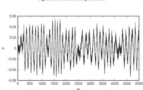
A set of training data was created by simulating the response of the system to a Gaussian white noise input. The resulting relative displacement (z) was then corrupted with Gaussian noise such that the signal to noise ratio of the signal was equal to 20 (Fig. 2). The mass was assumed known, such that the parameter vector to be estimated was

θ

¼ fc;k;k3g. The true parameter values and the chosen limits of the uniform prior distribution are shown inTable 1.

For the sake of demonstrating the potential benefits of studying the Shannon entropy of the training data, it is assumed here that the most probable parameter vector

θ

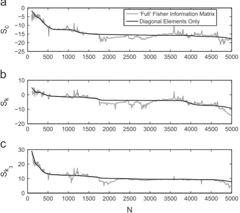
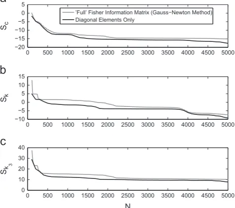
^is known. Firstly, the off-diagonal elements of the Fisher Information matrix were set to zero and the‘informativeness’of each parameter was approximated according to Eq.(22). Secondly, the entire Fisher Information matrix was approximated using finite difference methods and, in the same manner, the Shannon entropy of each parameter was evaluated. The resulting entropy estimates are plotted as a function of the number of data points in the training data inFig. 3.

The first point to note with regard toFig. 3is that the values obtained through computation of the full covariance matrix appear to be relatively noisy. This is because inverting the full Fisher Information matrix involves the combination of many more potentially erroneous gradient estimates than if one were to ignore the off-diagonal terms. This is compounded by the fact that estimation of the Hessian matrix requires the approximation of second-order derivatives using finite difference methods. In order to reduce the errors arising in this process, one can utilise the Gauss–Newton method[29]which allows the Hessian to be approximated using only first-order derivatives:

Hi;j2 ∑ N

n¼1

∂rn

∂

θ

i

∂rn

∂

θ

j

ð27Þ

wherern¼znz^nð

θ

Þ. Using this methodFig. 4shows that, relative to the results shown inFig. 3, the noise present in the

estimates made using the full Fisher Information matrix has been greatly reduced.

Fig. 5shows the estimated Shannon entropy–calculated using the determinant ofA(Eq.(21)). Specifically, the results

[image:7.544.217.337.421.506.2]

utilising the full Fisher Information matrix (calculated using the Gauss–Newton method) are compared to those obtained

Fig. 1.Base excited Duffing oscillator.

0 500 1000 1500 2000 2500 3000 3500 4000 4500 5000

−0.06 −0.04 −0.02 0 0.02 0.04 0.06

N

z

[image:7.544.149.398.518.674.2]

based on assumption of no parameter correlations. While, in this case, both methods produce fairly similar results, it is suggested that the Gauss–Newton method is the more general as its application is not limited to situations where parameter correlations are negligible.

Upon studying the Shannon entropy of each parameter,Figs. 3and4both indicate that if one were to use the first 4500 data points rather than the first 3500 data points of this specific set of training data, then one should realise a more

‘confident_’estimate of the parameterkbut still have similar levels of uncertainty with regard to the parameterscandk3.

To test this hypothesis two sets of MCMC simulations were run–one using the first 3500 data points and one using the first 4500 data points of training data. This was conducted using the Metropolis algorithm. Throughout this paper all MCMC simulations are conducted using the logarithm of the parameters so as to avoid scaling issues. The variances of the proposal densities were tuned such that acceptance ratio of the MH algorithm was roughly 40%.

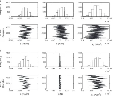
The resulting Markov chains are shown inFig. 6. It can be seen that, as predicted, by using the additional 1000 data points the uncertainty in the estimate fork has been reduced greatly while the uncertainty in the other parameters has remained relatively unchanged. Referring back to the training data (Fig. 2), it is interesting to note that it is not obvious exactlywhythis additional portion of training data has increased our confidence inkso drastically. This is an important result as it shows that plotting the Shannon entropy of the posterior can reveal features of the training data which may not be intuitively obvious.

4.2. Model selection

[image:8.544.37.505.78.130.2]

To investigate the issue of model selection, the response of the base-excited Duffing oscillator to a low amplitude excitation was analysed. This is because, at low amplitudes, the effect of the nonlinear term will be relatively small and so it may be possible to accurately replicate the response of the system over this region of the input space using a linear model. Consequently then, there are two competing model structures: one withk3(denotedM1) and one withoutk3(denotedM2). Table 1

True parameter values and chosen prior limits for parameter estimation of the base excited Duffing oscillator.

Parameter True value Lower prior limit Upper prior limit Unit

c 0.1 0 1 N s/m

k 50 0 1103

N/m

k3 1105 0 1107 N/m3

0 500 1000 1500 2000 2500 3000 3500 4000 4500 5000

−25 −20 −15 −10 −5 0

Sc

Sk

Sk

3

0 500 1000 1500 2000 2500 3000 3500 4000 4500 5000

−20 −10 0 10

0 500 1000 1500 2000 2500 3000 3500 4000 4500 5000

0 10 20 30

N

’Full’ Fisher Information Matrix Diagonal Elements Only

Fig. 3.Parameter estimation of the base-excited Duffing oscillator. The Shannon entropy for parameters (a)c, (b)kand (c)k3(evaluated using Eq.(22)).

[image:8.544.150.392.173.387.2]

The relative plausibility of the two model structures was measured using a Bayes Factor (computed using Eq. (26)):

β

1;2¼

PðDjM1Þ PðDjM2Þ

ð28Þ

such that a high value of

β

1;2indicates that the nonlinear model is more plausible than the linear model. The ability of the linear model to replicate the training data and a plot of ln

β

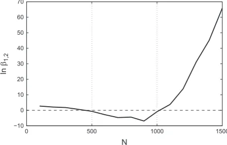
1;2as a function of the number of points in the training data are shown inFig. 7(a) and (b) respectively. It is clear that the plausibility of the nonlinear model relative to the linear model increases greatly when the ability of the linear model to replicate the training data worsens. Upon studyingFig. 8it is interesting to note that, if one had used between 500 and 1000 data points, it could have been incorrectly concluded that the linear model was preferable.

0 500 1000 1500 2000 2500 3000 3500 4000 4500 5000

−10 −5 0 5 10 15 20 25 30

N

S

[image:9.544.155.394.61.272.2]

’Full’ Fisher Information Matrix (Gauss−Newton Method) Diagonal Elements Only

Fig. 5.Parameter estimation of the base-excited Duffing oscillator. The Shannon entropy (evaluated using Eq.(21)) is presented. Grey lines represent

estimates using the full Fisher Information matrix (Gauss–Newton method) while black lines represent estimates made using only the diagonal elements of the Fisher Information matrix.

0 500 1000 1500 2000 2500 3000 3500 4000 4500 5000

−20 −15 −10 −5 0 5

Sc

0 500 1000 1500 2000 2500 3000 3500 4000 4500 5000

−10 −5 0 5 10 15

Sk

0 500 1000 1500 2000 2500 3000 3500 4000 4500 5000

0 10 20 30 40

N

Sk

3

[image:9.544.156.392.338.497.2]

’Full’ Fisher Information Matrix (Gauss−Newton Method) Diagonal Elements Only

Fig. 4.Parameter estimation of the base-excited Duffing oscillator. The Shannon entropy for parameters (a)c, (b)kand (c)k3(evaluated using Eq.(22)).

5. Example: system identification of the Tamar Bridge using model emulators

The Tamar Bridge, built in 1961, is situated in South West England. In 2001, in order to meet with EU directives the bridge was strengthened and widened. During this exercise a monitoring system that collects measurements of displacements, cable tensions and environmental conditions was installed in the interest of studying the bridge's performance during the

0.0960 0.098 0.1

500 1000 1500

Frequency

0.0960 0.098 0.1

2000 4000

c (Ns/m)

MCMC _Samples

49 49.5 50 50.5 51

0 500 1000 1500

49 49.5 50 50.5 51

0 2000 4000

k (N/m)

9.9 9.95 10 10.05

x 104 0

500 1000 1500

9.9 9.95 10 10.05

x 104 0

2000 4000

0.0960 0.098 0.1

500 1000 1500

Frequency

0.0960 0.098 0.1

2000 4000

c (Ns/m)

MCMC _Samples

49 49.5 50 50.5 51

0 500 1000 1500

49 49.5 50 50.5 51

0 2000 4000

k (N)

9.9 9.95 10 10.05

x 104 0

500 1000 1500

9.9 9.95 10 10.05

x 104 0

2000 4000

k3 (N/m3)

[image:10.544.78.469.57.390.2]

k3 (N/m3)

Fig. 6.Parameter estimation of the base excited Duffing oscillator. MCMC samples from the posterior distribution using (a) the first 3500 and (b) the first

4500 points of training data.

0 500 1000 1500 2000 2500 3000 3500 4000 4500 5000

−0.01 −0.005 0 0.005 0.01 z Training Data Linear Model

0 500 1000 1500 2000 2500 3000 3500 4000 4500 5000

−2000 0 2000 4000 6000 8000 10000 12000 N ln β1,2

Fig. 7. Selecting a model to replicate the response of the base-excited Duffing oscillator. (a) The ability of the linear model to replicate a set of training data.

[image:10.544.149.394.438.605.2]

upgrade. Nowadays the monitoring system has been extended to include dynamic measurements, and modal properties extracted from accelerometer measurements using stochastic subspace identification are available.

In order to better understand the dynamic response of the structure to environmental and operational conditions, a number of analyses have been carried out[30]. One such analysis utilised simple response surface models (employing linear regression) to capture the relationship between the extracted deck natural frequency and measured environmental and operational conditions (such as temperature, wind conditions and traffic loading). It was found that simple linear models (that may be thought of here as meta models) were able to account for the majority of the variation in the deck natural frequencies.

The question of model selection and informative training data is of much interest in this case, as a large database (which spans a number of years) is available for learning and contains numerous candidate parameters. The following analysis is concerned with using model emulators to predict the first natural frequency of the bridge specifically.

5.1. Parameter estimation

To begin the analysis it was hypothesised that the first natural frequency of the bridge (denoted

ω

) could be predicted using a model of the form:

^

ω

n¼

θ

Tn ð29Þ

where T represents the traffic load and

θ

is a parameter whose most probable value can be calculated through linear regression. In this case an improper prior and, as before, a Gaussian prediction-error model were utilised. Consequently, the likelihood is given by:

PðD

θ

;M¼ ð2

πσ

2_ÞN=2

exp 1 2

σ

2 ∑

N

n¼1

ð

ω

n

θ

TnÞ2

: ð30Þ

Differentiating the negative logarithm of Eq.(30)twice with respect to

θ

allows one to realise an exact expression forA:

A¼∑Nn¼1ðT 2 nÞ

σ

2 ð31Þ

and, as a result, an exact expression for the Shannon entropy of the posterior:

S_θ¼ln

σ

2

∑N n¼1ðTnÞ2

!

: ð32Þ

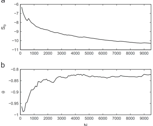
Interestingly, Eq.(32)implies that one can obtain more information about

θ

if the training data features large values ofT. To explain this one must recall that, through the choice of likelihood, it was assumed that each measurement was corrupted by the same level of noise. As a result Eq.(32)is essentially indicating thatinformative measurements are those which are far from the noise floor of the measurement process. As was pointed out in[24], this demonstrates a flaw in the definition of the likelihood as it assumes that the model will perform equally well over all regions of the input space. That being said,Fig. 9 shows that, in this case, Eq. (32) can be used to accurately determine which parts of the training data are the most informative with regard to the most probable estimate of

θ

.Fig. 10shows that there is a reasonably good match between the measured and modelled first natural frequency of the bridge.

0 500 1000 1500

−10 0 10 20 30 40 50 60 70

N

ln

[image:11.544.159.388.58.204.2]

β1,2

5.2. Model selection

In the final example, the issue of model emulator selection is investigated. A set of three candidate model structures are considered, the first is the‘traffic-only’model described in the previous section

^

ω

n¼

θ

1Tn: ð33Þ

The second model structure is:

^

ω

n¼

θ

1Tnþ

θ

2Wn ð34Þ

whereWrepresents wind speed, while the final model structure is:

^

ω

n¼

θ

1Tnþ

θ

2Wnþ

θ

3

τ

n ð35Þ

where

τ

represents temperature. Using the same training data as in the previous section, linear regression techniques were used to identify the most probable parameters of each model. These values and the mean square error (MSE) between the model and the training data are shown inTable 2. It can be seem that the reduction in MSE achieved using model 3 over model 2 seems relatively small compared to the reduction in MSE achieved using model 2 over model 1.

As inSection 4.2, the logarithm of the Bayes Factor was plotted as a function of the number of points in the training data. In this case the relatively simple structure of the models allowed the full Fisher Information matrix to be calculated analytically in a straightforward manner.

Fig. 11(a) shows the relative plausibility of model structure 2 relative to model structure 1. It is clear that using wind as an

additional input has made model 2 more plausible than model 1, and that this result becomes more pronounced as

0 1000 2000 3000 4000 5000 6000 7000 8000 9000

−11 −10 −9 −8 −7 −6

Sθ

0 1000 2000 3000 4000 5000 6000 7000 8000 9000

−1 −0.95 −0.9 −0.85 −0.8

N

[image:12.544.149.393.59.260.2]

θ

Fig. 9.(a) Shannon entropy of the posterior and (b) most probable parameter estimate for a traffic-dependent model of the first natural frequency of the

Tamar bridge.

2900 2950 3000 3050 3100 3150 3200 3250 3300

−2.5 −2 −1.5 −1 −0.5 0 0.5 1 1.5

N

[image:12.544.153.390.298.447.2]

ω

[image:13.544.35.508.77.132.2]

additional training data is used. However, upon studyingFig. 11(b), it is much less clear which out of models 2 and 3 are the more plausible. The key point here is that the relative plausibility of the two models does not become more pronounced as additional data is used. It would be incorrect to interpret this as meaning that model 2 is preferable to model 3. In fact it shows that this particular set of data does not contain enough information to help us to choose between models2 and3. Recalling that model 3 involves a temperature input it would be interesting to see if a relatively long set of training

Table 2

Most probable parameters and mean square error for 3 models of the first natural frequency of the Tamar bridge.

Model structure _θð1Þ

MP θ

ð2Þ

MP θ

ð3Þ

MP MSE

M1 0.8233 – – 0.3239

M2 0.8013 0.2322 – 0.2672

M3 0.7945 0.2226 0.0319 0.2666

0 1000 2000 3000 4000 5000 6000 7000 8000 9000

−1000 −800 −600 −400 −200 0 200

ln

β 1,2

0 1000 2000 3000 4000 5000 6000 7000 8000 9000

−25 −20 −15 −10 −5 0 5 10 15

N

ln

[image:13.544.44.440.79.358.2]

β 2,3

Fig. 11. The logarithms of Bayes Factor for (a) model structure 2 relative to model structure 1 and (b) model structure 2 relative to model structure 3.

2900 2950 3000 3050 3100 3150 3200 3250 3300

−4 −2 0 2 4

Training Data Model

2900 2950 3000 3050 3100 3150 3200 3250 3300

−4 −2 0 2 4

2900 2950 3000 3050 3100 3150 3200 3250 3300

−4 −2 0 2 4

N

ω

[image:13.544.158.397.390.614.2]

data–which included seasonal variations–would be more informative with regard to choosing between these two model structures. This is left as a topic of future work.

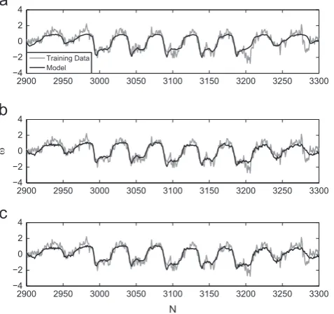
For the sake of completeness, the ability of the 3 models to replicate the first natural frequency of the bridge is shown in

Fig. 12.

6. Discussion and future work

With regard to model selection, it is assumed throughout this paper that one of the candidate model structures will be much more probable than the others and that, once identified, all future predictions will be made using this model. However, using a full Bayesian approach, one would make future predictions using every model in the set of candidates weighted by their posterior probabilities. This approach is discussed at length in[1]where it is described as‘hyper-robust predictions using model averaging’. The ability to improve one's‘hyper-robust’predictions using highly informative training data is certainly an interesting topic for future work. It may also be beneficial to see if the concepts detailed in this paper can be applied within the context of Bayesian structural health monitoring[31], in the Bayesian model selection of prediction error models[23]and the recently developed‘fast Bayesian FFT method’[32].

InSection 4the effect of the training data on one's confidence in individual parameter estimates was shown (Figs. 3and4).

This analysis was conducted using Eq.(22)–which is based on the assumption that one's parameter correlations are negligible. It is important to note that this will not always be true and that, in the general case, one should instead calculate the Shannon entropy using Eq.(21)(as shown inFig. 5).

Finally, it is again emphasised that the work presented here addresses the situation where one ispresentedwith a large set of training data–this is different from situations where one can easily generate more data using additional experimental tests. The latter situation was investigated by Metallidis et al. [26] where, with the aim of detecting faults in vehicle suspension systems by monitoring parameter estimates, the Shannon entropy was used to identify the experimental conditions which would lead to the greatest reduction in parameter uncertainty. It is interesting to note that, in[26], the optimum experiment was defined as that which revealed the most information about one's parameter estimates while, in the current paper, it is suggested that training data also needs to provide information with regard to model selection. A potentially useful avenue of future work could involve combining these ideas–the goal being to design experiments which are informative with regard to both model selection and parameter estimation.

7. Conclusions

This paper was concerned with the scenario where, with the aim of performing Bayesian system identification, one is presented with extremely large sets of training data. It addresses the situation where, through using a subset of the available data, one is able to make significant computational savings when running MCMC – something which is particularly important if one is constrained to using relatively expensive physics-based models. To that end, within the context of a Bayesian framework, an analytical expression approximating the effect of sets of training data on the posterior parameter covariance matrix was derived. This was then linked to previous work from the machine learning community in which the

‘informativeness’of training data was measured using the Shannon entropy of the posterior parameter distribution. With regard to the system identification of dynamical systems, it was then shown that the concepts developed in this paper can be used to select subsets of data which – with regard to both parameter estimation and model selection– are highly informative. Examples include the system identification of a base-excited Duffing oscillator using physics-based models and of model emulators which were used to predict the first natural frequency of the Tamar bridge.

Acknowledgments

This paper was funded by an EPSRC fellowship and the EPSRC Programme Grant‘Engineering Nonlinearity’EP/K003836/1.

References

[1]J.L. Beck, Bayesian system identification based on probability logic, Struct. Control Health Monit. 17 (7) (2010) 825–847. [2]D.J.C. MacKay, Bayesian interpolation, Neural Comput. 4 (3) (1992) 415–447.

[3]J.L. Beck, L.S. Katafygiotis, Updating models and their uncertainties. I: Bayesian statistical framework, J. Eng. Mech. 124 (4) (1998) 455–461. [4]J.S. Liu, Monte Carlo strategies in scientific computing, in: Springer Series in Statistics, Springer, New York, USA, 2008.

[5] R.M. Neal, Probabilistic Inference using Markov Chain Monte Carlo Methods, Technical Report, University of Toronto, 1993. [6]D.J.C. MacKay, Information Theory, Inference and Learning Algorithms, Cambridge University Press, New York, USA, 2003. [7]S. Kirkpatrick, C.D. Gelatt Jr., M.P. Vecchi, Optimization by simulated annealing, Science 220 (4598) (1983) 671–680. [8]H. Szu, R. Hartley, Fast simulated annealing, Phys. Lett. A 122 (3–4) (1987) 157–162.

[9]L. Ingber, Very fast simulated re-annealing, Math. Comput. Model. 12 (8) (1989) 967–973.

[10]P. Salamon, J.D. Nulton, J.R. Harland, J. Pedersen, G. Ruppeiner, L. Liao, Simulated annealing with constant thermodynamic speed, Comput. Phys. Commun. 49 (3) (1988) 423–428.

[12]J. Ching, Y.C. Chen, Transitional Markov Chain Monte Carlo Method for Bayesian model updating, model class selection, and model averaging, J. Eng. Mech. 133 (7) (2007) 816–832.

[13]J.L. Beck, K.M. Zuev, Asymptotically independent Markov sampling: a new Markov Chain Monte Carlo scheme for Bayesian inference, Int. J. Uncertain. Quantif. 3 (5) (2013).

[14]K. Worden, J.J. Hensman, Parameter estimation and model selection for a class of hysteretic systems using Bayesian inference, Mech. Sys. Signal Process. 32 (2012) 153–169.

[15]P.L. Green, K. Worden, Modelling friction in a nonlinear dynamic system via Bayesian inference, Top. Modal Anal. II 6 (2012) 657–667. [16]S. Duane, A.D. Kennedy, B.J. Pendleton, D. Roweth, Hybrid Monte Carlo, Phys. Lett. B 195 (2) (1987) 216–222.

[17]S.H. Cheung, J.L. Beck, Bayesian model updating using hybrid Monte Carlo simulation with application to structural dynamic models with many uncertain parameters, J. Eng. Mech. 135 (4) (2009) 243–255.

[18] Becker, K. Worden, J. Rowson, Bayesian sensitivity analysis of bifurcating nonlinear models, Mech. Sys. Sig. Process. 34(1), 57–75.

[19]P. Angelikopoulos, C. Papadimitriou, P. Koumoutsakos, Bayesian uncertainty quantification and propagation in molecular dynamics simulations: a high performance computing framework, J. Chem. Phys. 137 (14) (2012) 144103.

[20] H. Akaike, A new look at the statistical model identification, IEEE Trans. Autom. Control 19 (6) (1974) 716–723. [21]G. Schwarz, Estimating the dimension of a model, Ann. Stat. 6 (2) (1978) 461–464.

[22] J.L. Beck, K.V. Yuen, Model selection using response measurements: Bayesian probabilistic approach, J. Eng. Mech. 130 (2) (2004) 192–203. [23] E. Simoen, C. Papadimitriou, G. Lombaert, On prediction error correlation in Bayesian model updating, J. Sound Vibration, 332(18), 4136–4152. [24] D.J.C. MacKay, Information-based objective functions for active data selection, Neural Comput. 4 (4) (1992) 590–604.

[25] C. Papadimitriou, J.L. Beck, S. Kui Au, Entropy-based optimal sensor location for structural model updating, J. Vib. Control 6 (5) (2000) 781–800. [26] P. Metallidis, G. Verros, S. Natsiavas, C. Papadimitriou, Fault detection and optimal sensor location in vehicle suspensions, J. Vib. Control 9 (3–4) (2003)

337–359.

[27]C. Papadimitriou, Optimal sensor placement methodology for parametric identification of structural systems, J. Sound Vib. 278 (4) (2004) 923–947. [28] E.T. Jaynes, G.L. Bretthorst, Probability Theory: The Logic of Science, Cambridge University Press, New York, USA, 2003.

[29] Y. Bard, Nonlinear Parameter Estimation, Academic Press, New York, USA, 1974.

[30] E.J. Cross, K.Y. Koo, J.M.W. Brownjohn, K. Worden, Long-term monitoring and data analysis of the Tamar Bridge, Mech. Sys. Sig. Process. 35(1), 16-34. [31]M.W. Vanik, J.L. Beck, S.K. Au, Bayesian probabilistic approach to structural health monitoring, J. Eng. Mech. 126 (7) (2000) 738–745.