Pursuit-Evasion Problems with Linear Programming
.
White Rose Research Online URL for this paper:
http://eprints.whiterose.ac.uk/94359/
Version: Accepted Version
Proceedings Paper:
Qu, H., Kolling, A. and Veres, S.M. (2015) Computing Time-Optimal Clearing Strategies for
Pursuit-Evasion Problems with Linear Programming. In: Towards Autonomous Robotic
Systems. Lecture Notes in Computer Science, 9287 . Springer Verlag , pp. 216-228. ISBN
978-3-319-22415-2
https://doi.org/10.1007/978-3-319-22416-9_26
eprints@whiterose.ac.uk https://eprints.whiterose.ac.uk/
Reuse
Unless indicated otherwise, fulltext items are protected by copyright with all rights reserved. The copyright exception in section 29 of the Copyright, Designs and Patents Act 1988 allows the making of a single copy solely for the purpose of non-commercial research or private study within the limits of fair dealing. The publisher or other rights-holder may allow further reproduction and re-use of this version - refer to the White Rose Research Online record for this item. Where records identify the publisher as the copyright holder, users can verify any specific terms of use on the publisher’s website.
Takedown
If you consider content in White Rose Research Online to be in breach of UK law, please notify us by
pursuit-evasion problems with linear
programming
⋆Hongyang Qu, Andreas Kolling, and Sandor M. Veres
Dept. of Automatic Control and Systems Engineering, University of Sheffield, UK
{h.qu,a.kolling,s.veres}@shef.ac.uk
Abstract. This paper addresses and solves the problem of finding op-timal clearing strategies for a team of robots in an environment given as a graph. The graph-clear model is used in which sweeping of locations, and their recontamination by intruders, is modelled over a surveillance graph. Optimization of strategies is carried out for shortest total travel distance and time taken by the robot team and under constraints of clearing costs of locations. The physical constraints of access and timely movements by the robots are also accounted for, as well as the ability of the robots to prevent recontamination of already cleared areas. The main result of the paper is that this complex problem can be reduced to a computable LP problem. To further reduce complexity, an algorithm is presented for the case when graph clear strategies are a priori available by using other methods, for instance by model checking.
1
Introduction
Search and pursuit-evasion problems appear in a variety of formulations in the literature. A survey of methods can be found in [2] where taxonomies of ap-proaches and assumptions based on attributes of searchers, targets and the envi-ronments are reviewed. A large class of problems assumes that there is a graph-based description, an “abstraction”, of the environment which models it into locations, represented by vertices, and passages between locations, represented by the edges of a graph. Once such an abstraction is available one can apply the techniques developed in graph-searching for robotic search. Probably the first related analysis of graph searching has been published in [12]. The searchers’ objective was to catch evaders along the edges the graph with the minimum number of searchers. A large number of variants of graph searching problems appeared which differed in their assumption on the mobility and cost models of a team of search robots clearing edges and vertices of a graph. A review of these is found in [3]. Many of the methods and results developed in the con-text of graph-searching were primarily concerned with minimizing the number of searchers rather than the distance or time travelled. In this paper we present
a solution for minimizing time, in addition to the number of searchers, using an linear programming formulation for a graph-based pursuit-evasion problem.
The recent framework of interest in this paper is the Graph-Clear(GC) model [5, 7, 10] for pursuit-evasion problems with teams of robots. GC is particular useful for search problems where multiple robots cooperate to detect intruders in complex environments with limited sensing capabilities. Following the GC approach, in this paper we consider the problem of searching a graph for an unknown number of omniscient and smart targets moving with unbounded speed. Such targets represent a worst-case scenario and are represented by the formal concept of contamination [12], defined in Section 3. The searchers can execute actions that clear contamination or block it from spreading through parts of the environments. These actions have an associated cost that reflects the number of robots needed to prevent targets from passing through undetected.
Linear programming (LP) techniques have previously been applied to robot pursuit-evasion problems in [14] and [13]. In [14] the authors considered polygo-nal environments partitioned into convex regions. From a region a searcher is able to detect targets in all other visible regions. The resulting visibility relations be-tween regions are considered in the LP formulation. Searchers can move bebe-tween adjacent regions at each time step but, to reduce the complexity, multiple pur-suers cannot occupy the same region. A receding horizon approach was applied in order to solve the LP formulation, albeit without guarantees for optimality. Our work presented here is a continuation of [13] which considered the computa-tion of strategies for Graph-Clear with the minimal number of searchers using an LP formulation. In this paper we focus on computing time optimal strategies. In contrast to [14] target detection in our scenario may require multiple searchers and our environmental model is a graph with vertices that do not necessarily represent convex regions and can exhibit more complex neighborhood relations. In general, the problem of computing time optimal strategies is shown to be harder than minimizing the number of searchers [1], e.g., it is already NP-hard on star-shaped trees.
In the next section a formal description of surveillance graphs and of the GC problem is provided. Section 3 develops the LP model to obtain minimal total travel time of the robots to clear a graph in a physically feasible way. Section 4 deals with optimisation heuristics to reduce the computational complexity of the optimal strategy. Section 5 applies the LP system to find the shortest execution plan for a given clear strategy. Section 6 presents a computational example and the last section concludes the paper.
2
Pursuit-Evasion problem
For our purposes we adopt the model called Graph-Clear introduced and formal-ized in [10]. Therein the environment is given by a surveillance graph which is a weighted graphG= (V, E, w) with an undirected graph with vertex setV, edge set E, andw:V ∪E→N+ as a weight function. To model contamination and
either being clearor contaminated and edges either being clear, contaminated, or blocked. These are abbreviated asR,C, and B for clear, contaminated, and blocked, respectively. The state of the surveillance graph withnvertices andm
edges is then given by ν ∈ V(G) ={R,C}n× {R,C,B}m. As a shorthand, we write ν(vi) and ν(ej) for the state of a particular vertex or edge. Contamina-tion spreads on recontaminaContamina-tion paths. These are paths of vertices and edges on which no edge is blocked. Finally, searchers can execute actions which are either a sweep on a vertex or a block on an edge. The executed actions on G
can be represented bya={a1, . . . , an+m} ∈ {0,1}n+m=A(G) where a 1 for an associated vertex indicates a sweep and a 1 for an associated edge indicates a block. The cost of an actionais given byc(a) =Pin=1aiw(vi)+P
m
j=1an+jw(ej), representing the number of robots needed to execute all sweeps and blocks for the action. The spread of contamination and the clearing of actions can now be formalized via a transition function ζ, defined in [10] as follows:
Definition 1 (Transition function). Let G, V(G) and A(G) be defined as
above. The transition functionζ maps a state and an action into a new state:
ζ:V(G)× A(G)→ V(G).
Given a∈ A(G) andν∈ V(G), the new stateν′ is defined as follows:
1. ifan+j= 1,1≤j≤m, thenν′(ej) =B 2. ifai= 1,1≤i≤n, thenν′(vi) =R
3. ifνn+j =B,an+j = 0,1≤j≤m, and no recontamination path betweenej andx∈V ∪E with ν(x) =C exists, then ν′
n+j=R
4. if there exists a recontamination path betweenx∈V ∪Eandy∈V∪E with
ν(y) =C, thenν′(x) =C 5. ν′
i=νi otherwise.
In colloquial terms the above describes the following rules stated in [10]:
1. edges where a block action is applied become blocked; 2. vertices where a sweep action is applied become clear;
3. blocked edges where a block action is not applied anymore become clear if there is no recontamination path involving them;
4. vertices or edges for which a recontamination path towards a contaminated vertex or edge exists become contaminated;
5. vertices or edges keep their previous state if none of the former cases apply.
A strategy to clear an initially fully contaminated surveillance graph G is a sequence of actions S ={a1, a2, . . . , ak}. A strategy that is a solution to the Graph-Clear problem has in addition a minimal cost, i.e.ag(S) = maxi=1...kc(ai) is minimal. In [10] it has been shown that solving the Graph-Clear problem on graphs is NP-hard and a polynomial time algorithms for trees was presented. The algorithms has been applied to robotic search in [6, 8–11]. In [6] a method to extract instances of the Graph-Clear problem from robot maps was presented, validating the graph-based model for practical use.
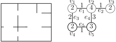
connections between rooms. Edges between vertices are blocked by placing a robot in the connection between rooms. All contaminated parts can hide an intruders while cleared parts are guaranteed to be free of undetected intruders. A room is cleared by using the specified number of robots to sweep through it.
v
5
.
1
1
4
1
2
3
2
2
3
2
e
3e
4v
1v
2v
3e
1e
2e
5v
4 [image:5.612.207.408.185.259.2]
Fig. 1.A simple example environment and a possible surveillance graph that can model the search for a target. Numbers on vertices are clearing costs and numbers on edges are blocking costs.
Much of the prior work in graph-searching by [3] focused on actions that are executed by a single searcher, while the Graph-Clear model explicitly considers actions that require multiple searchers. In this paper we consider connected searching (sometimes also named as contiguous search) to be a search in which the cleared edges and vertices always form a connected subgraph. In Graph-Clear, it is obligatory to block every connected edge when sweeping a node.
Fig. 2 presents a surveillance strategy to solve the Graph-Clear problem associated with the graph shown in Fig. 1. The first column displays the status of the graph in the form of “ν(v1)· · ·ν(v5)ν(e1)· · ·ν(e5)”, the second the applied
action of the form “av1· · ·av5 ae1· · ·ae5”, and the third the cost. In the third row an action sweeps two vertices at the same time. A final action removing all blocks is executed in the end (with 0 cost). The cost of this strategy is 12, i.e., the maximum value read in the third column, and as such not optimal.
ν(G) a c(a)
CCCCC CCCCC 10000 10100 5
RCCCC BCBCC 00010 10101 6
RCCRC BCBCB 01100 11011 12
RRRRC BBRBB 00001 00011 7
RRRRR RRRBB 00000 00000 0
[image:5.612.230.386.479.561.2]RRRRR RRRRR
Fig. 2.A Graph-Clear strategy.
3
Strategy with global minimal execution time
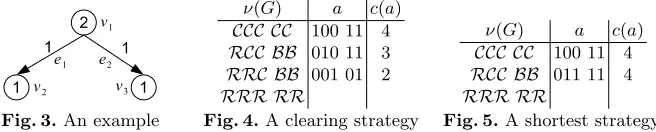
that have the shortest execution time. For example, Fig. 4 shows an optimal strategy for the model in Fig. 3. Fig. 6 illustrates an execution of the strategy
1
1 1
v1
1 2
v3
v2
[image:6.612.145.473.163.229.2]e1 e2
Fig. 3.An example
ν(G) a c(a)
CCC CC 100 11 4
RCC BB 010 11 3
RRC BB 001 01 2
RRR RR
Fig. 4.A clearing strategy
ν(G) a c(a)
CCC CC 100 11 4
RCC BB 011 11 4
RRR RR
Fig. 5.A shortest strategy.
in Fig. 4 with 4 robots. In this figure, two robots are marked with solid discs and the other two are marked by circles. Clearly, this graph does not represent the shortest solution because step 2 can be skipped by asking the two robots marked with solid discs in v1 in Fig. 6(b) to move with the other two at the
same time. This would make the system evolve from step 1 in Fig. 6(b) to step 3 directly in Fig. 6(d). Indeed, by skipping step 2, we change this strategy into
v1
v3 v2
e1 e2
(a) Initial location
v1
v3 v2
e1 e2
(b) Step 1
v1
v3 v2
e1 e2
(c) Step 2
v1
v3 v2
e1 e2
[image:6.612.138.480.335.396.2](d) Step 3
Fig. 6.An execution of a clearing strategy
a new strategy demonstrated in Fig. 5.
In this section, we propose a linear programming system to compute a clear-ing strategy that has the minimal cost and its execution plan for each robot with minimal execution time. We first present the general constraints that can be ap-plied in a broader context, and second the specific constraints for computing the shortest execution path. We assume that all robots move at the same speed, and therefore, execution time in one step can be measured by the maximum travel distance during the step. We also assume that the distance between a vertex and an adjacent edge is constant.
3.1 General constraints
As stated in the previous section, a graph with nvertices andm edges can be cleared innsteps, each of which clears one vertex. Suppose that at leastkrobots are needed to clear a graph1. In each step, a robot can be located in one of the
n+mplaces. Letl=n+mbe the number of possible locations. We also assume that initially the robot has been placed into a vertex or edge. Therefore, we need
l·(n+ 1) binary LP variablesX1, . . . , Xl·(n+1) to encode all possible locations
of each robot in every step and the initial locations. We assume that the edges
1
are numbered after vertices, i.e., fromn+ 1 ton+m, and that the robots are numbered from 0 to k−1. The initial location of robot j (0 ≤j ≤k−1) is constrained by the following equation:
Xj·l+1+· · ·+X(j+1)·l= 1. (1)
As each variable is binary, the above equation captures the fact that the robot locates exactly in one place.
The constraint for the location of robot j at the i-th step (1 ≤ i ≤ n) is formulated as follows.
Xi·k·l+j·l+1+· · ·+Xi·k·l+(j+1)·l= 1. (2) The expressioni·k·labove indicates the total number of LP variables from step 0 to stepi−1, where the initial location is seen as step 0. We call the variables appearing in Equations (1) and (2)location variables. Asnsteps are required to clear the graph, there are
∆1= (n+ 1)·k·l (3)
location variables in the LP system forkrobots.
The following constraint models the travel distance of a robot moving in a step. For a robotjand two locationspandq(1≤p, q≤l), we generate a binary LP variableXf(p,q) to represent the possibility that the robot moves frompto
qat thei-th step (1≤i≤n).
2·Xf(p,q)−X(i−1)·k·l+j·l+p−Xi·k·l+j·l+q≤0, (4) where
f(p, q) =∆1+ (i−1)·k·l2+j·l2+ (p−1)·l+q. (5)
In this constraint, X(i−1)·k·l+j·l+p encodes the location of the robot j at the (i−1)-th step andXi·k·l+j·l+q its location at thei-th step. When both variables are set to one, which means that indeed the robot moves from p to q at the
i-th step,Xf(p,q), a binarymove variable, can be set to one without violation of
Equation (4). In other cases, i.e., at least one location variable is zero, Xf(p,q)
has to be set to zero, indicating that this is not an actual move. For each robot and each step, there arel2possible moves, and hence, we needl2move variables. The following constraint requires that exactly one of thel2move variables is set
to one representing the actual move. X
1≤p,q≤l
Xf(p,q)= 1. (6)
The move variables constitute the majority of total variables used in the LP system: there are
∆2=n·k·l2 (7)
move variables.
Now we introducedistance variables of integer type, one for each step. Let
Dibe the distance variable for thei-th step (1≤i≤n). As each robot has one move variable set to one, the following constraint states thatDi is no less than the maximum distance a robot can move in one step:
^
0≤j<k
{( X
1≤p,q≤l
wheredp,q is the minimum travel distance between pandq. Clearly, there are
∆3=n (9)
distance variables. The objective function is to minimise the sum of the distance variables, i.e.,
X
1≤i≤n
Di. (10)
3.2 Constraints for Graph-Clear strategies
In this subsection, we model the constraints required by Graph-Clear strategies. The first constraint is to block an edge. Letcer be the cost of edgeer(1≤r≤m). At thei-th step, edgeer has a binaryedge blockingvariableYi·m+rto represent whether it is being blocked at this step. Equation (11) enforces that the edge blocking variable cannot be set to one if the number of robots staying in the edge is fewer than the cost of blocking the edge.
cer·Yi·m+r− X
0≤j<k
Xi·k·l+j·l+n+r≤0. (11)
There are in total
∆4=n·m (12)
of edge blocking variables. Equation (13) guarantees that the edge blocking vari-able is set to one as far as the number of robots in the edge reaches the required number for blocking the edge.
k−1
X
j=0
Xi·k·l+j·l+n+r+ (cer−1−k)·Yi·m+r≤cer−1. (13)
The correctness of Equation (13) can be proved by contradiction. Suppose the number of robots in the edge is large enough to block the edge and the edge blocking variable is set to zero. Then, Equation (13) is transformed into
k−1
X
j=0
Xi·k·l+j·l+n+r≤cer−1,
which is clearly unsatisfiable. Therefore, Yi·m+r has to be set to 1 and Equa-tion (13) becomes
k−1
X
j=0
Xi·k·l+j·l+n+r≤k,
which is tautology.
Clearing a vertex at thei-th step can be modelled in a similar way. Letcvr be the cost of clearing vertex vr (1 ≤ r ≤ n), and Zi·n+r the binary vertex clearingvariable. Equations (14) and (15) formalise the constraint. In addition, all adjacent edges tovrhave to be blocked at the same time. For each adjacent edgees, Equation (16) requestsesto be blocked.
cvr·Zi·n+r− X
0≤j<k
k−1
X
j=0
Xi·k·l+j·l+r+ (cvr−1−k)·Zi·n+r≤cvr−1. (15)
Zi·n+r−Yi·m+s≤0. (16)
There are in total
∆5=n2 (17)
of vertex clearing variables.
A Graph-Clear strategy clears one vertex at each step, which can be expressed as follows.
n X
r=1
Zi·n+r≥1. (18)
The above equation states that at thei-th step, there exists a noder(1≤r≤n) that is being cleared. When a Graph-Clear strategy is executed completely, we would expect that all vertices have been cleared, which is expressed by the following equation on all vertices: for each noder, there exists a stepi(1≤i≤n) at whichris cleared.
n X
i=1
Zi·n+r≥1. (19)
The strategy also requires that the node being cleared at thei-th step (i >1) should be adjacent to a node that has been cleared at a previous step. Let
Vr={r1,· · ·, rt}be the set of indices of adjacent nodes for node vr. We have
Zi·n+r− i−1
X
j=1
X
p∈Vr
Zj·n+p≤0. (20)
The correctness of Equation (20) is obvious: Zi·n+r cannot be set to 1 if none of Zj·n+p variables is 1, representing no adjacent nodes in Vr has been cleared before. Similarly, an edgeer cannot be blocked at thei-th step until one of its adjacent vertices has been swept before or being swept at the same step. Let
Er={r1, r2}be the adjacent vertices ofer. We have
Yi·m+r− i X
j=1
X
p∈Er
Zj·n+p≤0. (21)
To prevent recontamination, an edgeerthat is blocked for sweeping a vertex has to be continuously blocked until both adjacent vertices have been swept. Let
vp be an adjacent vertex ofer. This constraint is characterised by the equation:
Y(i−1)·m+r− i X
j=1
Zj·n+p−Yi·m+r≤0. (22)
The correctness of Equation (22) is straightforward: at thei-th step,Yi·m+rhas to be set to 1, meaning thater is being blocked at this step, if it is blocked at the previous step (Y(i−1)·m+r= 1) and vertex vp has not been swept yet (all Z variables are zero). If one of the Z variable is 1, then there is no constraint on
Complexity The total number of LP variables is
∆=∆1+∆2+∆3+∆4+∆5, (23)
where ∆2 is in the dominant position, which means that the number of LP
variables is proportional to O(k×n×(n+m)2). This suggests that the LP
program for a large surveillance graph can easily be beyond the capacity of the state-of-the-art LP solvers.
4
Optimisation heuristics
Equation (1) allows the robots to be scattered all over the graph when they start to clear the graph. A reasonable assumption in practice is to place them in a vertex initially. Therefore Equation (24) can be modified to exclude edges.
Xj·l+1+· · ·+Xj·l+n= 1. (24)
Similarly, we can assume all robots initially gather in an edge if requested. After taking Equation (24), we could make another assumption that all robots start from the same location. This can be modelled by the following constraints: for all vertex 1≤i≤nand all robots 0< j < k, we have
Xi−Xj·l+i= 0. (25)
The equations in this category set all variables corresponding to the same initial location to the same value by letting all robots from 1 tok−1 stay in the same location of robot 0.
To speed up the search for an optimal clear strategy with shortest execution time, it is essential to get a tight upper-bound for each distance variables. If all robots are initially positioned in the same vertex, then it is reasonable to assume they would sweep the initial vertex first. Therefore, the shortest time to execute the first step is the same as the time for some robots moving to the adjacent edges to block. Constraints specified in Equations (6) and (8) can be simplified by removing impossible moves between vertices and edges. For example, suppose that robots initially gather at vertexv3 in Fig. 1. To sweepv3, there is no need
to allow robots to move to vertexv2 and beyond. Hence, the move variables for
those unrealistic moves can be removed from Equations (6) and (8).
For other steps, it is also very helpful if we can estimate the maximum dis-tance that a robot needs to move. For the example in Fig. 1, we can get an optimal execution even if we do not allow a robot to move across three edges if it starts from an edge, or across three vertices if it starts from a vertex. For example, a robot cannot move frome2 toe3 or fromv2 tov4 in one step.
5
Executing a predefined strategy with minimal
execution time
vertex to sweep and edges to block at each step, and thus, greatly reduces the search space. To achieve this, the constraints listed in Section 3.2 are not needed any more. Instead, we add the following constraints.
As in the previous section, we assume that initially the robots stay in the vertex that is swept at the first step. For each edgeer being blocked at thei-th step, we generate the following inequality.
n X
j=1
Xi·n·l+j·l+n+r≥cer. (26)
Similarly, for vertexvr being swept at thei-th step, we have n
X
j=1
Xi·n·l+j·l+r≥cvr. (27)
The intuition in these equations is that the number of robots in er (vr) should exceed the cost of blockinger(sweepingvr).
Note that the LP system does not impose any constraints on edges that are in the clear, i.e.,R, state. A clear edge may still be blocked during the execution when necessary for saving execution time.
Complexity The extra constraints in Equations (26) and (27) do not introduce
new LP variables. Thus, the total number of LP variables for computing the execution of a predefined strategy is
∆=∆1+∆2+∆3. (28)
This suggests that the complexity for finding an optimal execution plan for a given strategy is in the same level of that for computing a global optimal exe-cution plan. In practice, however, this kind of LP programs can be solved much faster than that in Section 3 due to fewer LP variables and more constraints.
6
Experiment
The LP system described in this paper can be automatically generated by pro-viding the adjacency matrix of the graph, and the distance matrix which records the minimal travel time/distance between any two locations in the graph. The number of robots, i.e., the cost of clearing a graph, also needs to be specified. In [13], we proposed to apply model checking techniques to compute the minimal cost and generating a corresponding strategy. Fig. 7 shows such a strategy.
location at step 0 is the initial location. The last column gives the number of time units needed for every step.
ν(G) a c(a)
CCCCC CCCCC 00001 00011 7
CCCCR CCCBB 00010 00111 8
CCCRR CCBBB 10000 10110 8
RCCRR BCBBR 01000 11010 9
RRCRR BBRBR 00100 01000 3
[image:12.612.142.481.164.271.2]RRRRR RBRRR
Fig. 7.A Graph-Clear Strategy.
Step Robot Time
1 2 3 4 5 6 7 8 9 0 v5 v5 v5 v5 v5 v5 v5 v5 v5
1 v5 e5 v5 e5 e4 e4 e4 v5 e5 1
2 v4 e3 e4 e3 e4 e1 e4 e5 v4 2
3 e3 v1 e4 v1 e4 e1 e4 v5 e3 1
4 v2 v2 e4 e1 e4 e2 v2 e4 v2 3
5 e2 v2 e4 e1 e4 v3 e2 e4 v3 2
Fig. 8.An execution
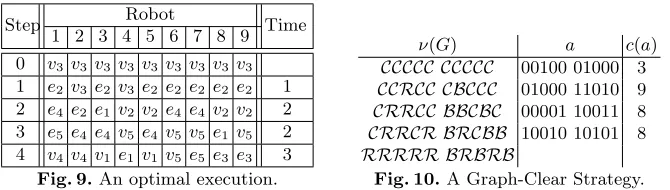
However, if we use the LP system defined in Section 3 and the heuristics in Section 4, then the solver managed to find an execution plan with 8 time units. The locations at each step is listed in Fig. 9 and the corresponding strategy is shown in Fig. 10. We can see that vertices v1 and v4 can be cleared in one
step, which makes the fifth step redundant. However, the time for solving the LP system was increased to 60143 seconds.
Step Robot Time
1 2 3 4 5 6 7 8 9 0 v3 v3 v3 v3 v3 v3 v3 v3 v3
1 e2 v3 e2 v3 e2 e2 e2 e2 e2 1
2 e4 e2 e1 v2 v2 e4 e4 v2 v2 2
3 e5 e4 e4 v5 e4 v5 v5 e1 v5 2
[image:12.612.141.476.371.466.2]4 v4 v4 v1 e1 v1 v5 e5 e3 e3 3
Fig. 9.An optimal execution.
ν(G) a c(a)
CCCCC CCCCC 00100 01000 3
CCRCC CBCCC 01000 11010 9
CRRCC BBCBC 00001 10011 8
CRRCR BRCBB 10010 10101 8
RRRRR BRBRB
Fig. 10.A Graph-Clear Strategy.
Discussion.During at any point of the process of solving the LP system, Gurobi
solver to solve the LP system for the global optimal solution and terminate the solving process at any point when a better strategy than the known strategy is found.
7
Conclusion
This paper solves the optimal design of movements by robots in an enviroment modelled by a surveillance graph under the constraints of robot movements and resources. A method to find a shortest execution plan for a given clear strategy is also presented. It is assumed that the moving distance between a vertex and an adjacent edge is constant. As this assumption may not hold in practice when a vertex represents a fairly large area, further work can be carried out to improve the modelling approach taken in this paper.
References
1. R. Borie, C. Tovey, and S. Koenig. Algorithms and complexity results for pursuit-evasion problems. InProceedings of the International Joint Conference on Artificial Intelligence, pages 59–66, 2009.
2. T.H. Chung, G.A. Hollinger, and V. Isler. Search and pursuit-evasion in mobile robotics. Autonomous Robots, 31(4):299–316, 2011.
3. F. V. Fomin and D. M. Thilikos. An annotated bibliography on guaranteed graph searching. Theoretical Computer Science, 399(3):236–245, 2008.
4. Gurobi Optimization, Inc. Gurobi optimizer reference manual, 2014.
5. A. Kolling and S. Carpin. The graph-clear problem: definition, theoretical proper-ties and its connections to multirobot aided surveillance. Proc. of IEEE/RSJ Intl. Conf. On Intelligent Robots and Systems, pages 1003–1008, 2007.
6. A. Kolling and S. Carpin. Extracting surveillance graphs from robot maps. In
Proceedings of IROS’08, pages 2323–2328, 2008.
7. A. Kolling and S. Carpin. Multi-robot surveillance: an improved algorithm for the graph-clear problem. Proc. IEEE Int. Conf. on Robotics and Automation, pages 2360–2365, 2008.
8. A. Kolling and S. Carpin. Surveillance strategies for target detection with sweep lines. InProceedings of IROS’09, pages 5821–5827, 2009.
9. A. Kolling and S. Carpin. Multi-robot pursuit-evasion without maps. In Proceed-ings of ICRA’10, pages 3045–3051, 2010.
10. A. Kolling and S. Carpin. Pursuit-evasion on trees by robot teams. IEEE T. Robot., 26(1):32–47, 2010.
11. A. Kolling and A. Kleiner. Multi-uav motion planning for guaranteed search. In
Proceedings of AAMAS’13, pages 79–86, 2013.
12. T.D. Parsons. Pursuit-evasion in a graph. In Y. Alavi and D. R. Lick, editors,
Theory and Applications of Graphs, volume 642, pages 426–441. Springer, 1976. 13. H. Qu, A. Kolling, and S. M. Veres. Formulating robot pursuit-evasion strategies
by model checking. InProceedings of IFAC’14, pages 3048–3055, 2014.