The use of Fourier analyzed square waves in the determination of the modulation transfer function of photographic materials

Rochester Institute of Technology

RIT Scholar Works

Theses

Thesis/Dissertation Collections

1978

The use of Fourier analyzed square waves in the

determination of the modulation transfer function

of photographic materials

David Moffett

John Stanton

Follow this and additional works at:

http://scholarworks.rit.edu/theses

This Senior Project is brought to you for free and open access by the Thesis/Dissertation Collections at RIT Scholar Works. It has been accepted for

inclusion in Theses by an authorized administrator of RIT Scholar Works. For more information, please contact

[email protected].

Recommended Citation

THE

USE

OF

FOURIER ANALYZED SQUARE

WAVES

IN

THE

DETERMINATION

OF

THE

MODULATION

TRANSFER FUNCTION

OF

PHOTOGRAPHIC

MATERIALS

by

David

Moffett

and

John

Stanton

A

thesis

submitted

in

partial

fulfillment

of

the

requirements

for

the

degree

of

Bachelor

of

Science

in

the

School

of

Photographic

Arts

and

Sciences

in

the

College

of

Graphic Arts

and

Photography

of the

Rochester

Institute

of

Technology

March

1978

-TABLE

OF

CONTENTS

Introduction

pg

1

Theory

pg

3

Experimental

pg

]k

Discussion

pg

21

Conclusions

pg

31

LIST OF FIGURES

1.

MTF

-

Typical

_and

the

Ideal

pg

3

2.

Cascading

MTF

Curves

pg

k

3.

Application

of

MTF

Curves

pg

5

4.

Sinusoidally Varying

Transmission

Distribution

pg

7

5.

Transmission

Distribution

of a

Symmetrical

Square

Wave

pg

10

6.

Transmission

Distribution

of a

Symmetrical

Square Wave

and

Its

First

Harmonic

7.

Master

Square Wave

Target

8.

MTF

-

Conventional

_and

Square Wave

Methods

9.

Characteristic

Curve

-

Kodak

Fine

Grain

Aerial

Duplicating

Film

Type

2430

10.

Characteristic

Curve

-

Rochester

Film

Co.

Type

3T

Reversal

Microfilm

11.

Characteristic Curve

-

Rochester

Film

Co.

Type

1K

Microfi 1m

12.

Characteristic

Curve

-

Intermediate

Square

Wave

Target

13.

Characteristic

Curve

-

Final

Square

Wave

Target

14.

Microdensitometer

Calibration

Curve

-Sinusoidal

Target

15.

Microdensitometer

Calibration

Curve

-Sinusoidal

Sample

pg

12

pg

20

pg

27a

pg

35

pg

36

pg

37

pg

38

pg

39

pg

40

LIST

OF

FIGURES,

CONT.

16.

Microdensitometer

Calibration

Curve

-Square

Wave

Target

pg

42

17.

Microdensitometer

Calibration

Curve

-Square

Sample

pg

43

18.

Conventional

MTF

-

Target

imaged

_at

IX

reduction with no mask

pg

44

19.

Conventional

MTF

-

Target

imaged

_at

4X

reduction with no mask

pg

45

20.

Conventional

MTF

-

Target

imaged

_at

4X

LIST

OF TABLES

1.

A

Typical

Set

of

Frequencies

Used

to

Determine MTF

2.

Square Wave

Frequencies

and

Their

Harmonics

3.

Frequencies

of

Sinusoidal

Target

4.

Computer

Output

Sample

5.

Frequencies

of

Sample

with

Harmonics

6.

Frequencies

of

the

Square

Wave

Target

and

Sample

7.

Processing

Data

for

Figures

8

Through

20

8.

Equations

of

the

Microdensitometer

Calibration

Curves

pg 48

pg

9

pg

13

pg

14

pg

24

pg

26

pg

30

ACKNOWLEDGEMENTS

A

special

thanks

is

extended

to

Professor

Mohamed

F.

Abouelata

for

his

patient

help

and

inspiration

throughout

this

project.

Thanks

also go

to

Todd

Calvin

and

Russell

Schuter

of

the

Rochester

Film

Company,

the

faculty

and staff of

the

Photographic

Science

department

ABSTRACT

Fourier

analysis and a computer were used to generate

the

Fourier

series and coefficients

for

the

transmission

distribution

of a square wave target and

the

effective

exposure produced on

Kodak

Plus-X

film.

This

was performed

in

an effort

to

find

a workable alternative to the pro

posed

American

National

Standards

Institue

(ANSI)

method

for

the

determination

of the photographic modulation

transfer

function.

The

results showed that the square

wave method generated a curve with the same general trend

as the conventional

ANSI

method.

The

Fourier

analyzed

square wave method

had

a greater

degree

of

variability

than

did

the standard method.

The

square wave

targets

used

for

the

determination

were manufactured at the

Roch

INTRODUCTION

The

widespread acceptance of

the

modulation transfer

function

(MTF)

as a means of

describing

the

band

limitations

of photo-optical systems

has

raised

interest

in

its

deter

mination.

The

American

National

Standards

-Institute

has

set

forth

a rigorous procedure

for

its

determination.

This

method utilizes targets

varying

sinusoidally

in

transmission,

over a range of

frequencies.

The

modulation

of the output

distribution

is

divided

by

the

input

and

plotted as a

function

of spatial

frequency,

which generates

the

MTF

curve.

This

procedure

is

lengthy

as compared to

the square wave method which

is

the subject of this project.

Fourier

mathematics,

long

used

in

the physical

sciences,

can

be

applied to the problem of

MTF

determination.

Fourier

mathematics

breaks

a periodic

function

such as a square

wave,

into

an

infinite

set of

harmonic

components.

Incorporating

the two aforementioned

concepts,

the

photographic

MTF

of

Kodak

Plus-X

film

was

determined.

Both

the conventional

(sinusoidal)

and square wave methods were

as

the

conventional method

but

with a

higher

noise

level.

The

eight square wave targets used were

bar

targets

imaged

onto

film.

The

sinusoidal target used contained

19

freq

uencies.

The

proposed

ANSI

standard was

followed

or adapted

to

the

square wave method.

Due

to

apparatus

restrictions,

the

tests

were aimed at the

lower

frequencies

(0

to

40

cycles

THEORY

The

modulation transfer

function

(MTF)

is

a quanti tative and graphical

description

of the performance of an optical and/or

imaging

system over a range of spatial

frequencies.

The

MTF

is

a useful measure

Of

the

effects of

light

scatter and absorption within the emulsion

during

exposure and chemical

dynamics

of photographic

development.

A

perfect system

would,

if

it

existed,

reproduce small as well as

large

subject areas with equal

fidelity.

Such

a system would

have

a

flat

response at a

level

of

1.0

or

at a modulation equal to

100%.

100

%

modulation

spatial

frequency

Since

all physical systems are

band

limited

and possess

inherent

noise,

input

signals are

diminished

or

distorted.

This

results

in

a

loss

of

image

clarity

and modulation.

As

the spatial

frequency

increases,

the

loss

of modulation

increases

and

clarity

decreases.

Modulation

transfer

function

curves are useful

in

selecting

photographic materials and optical components

for

a number

of professional applications.

In

a

linear

system,

MTF

curves can

be

cascaded so that a model can

be

visualized.

This

cascading

is

equivalent to point

by

point multiplication

and

is

a useful approximation to the

final

system

MTF.

MTF

MTF

film

lens

MTF

system

[image:12.571.82.524.401.544.2]

Modulation

transfer

function

curves can

be

utilized

to

select

the

best

material

for

a

job

if

the

frequency

range needed

is known.

This

capability

surpasses

resolving

power which

only

establishes an upper

limit

of

frequency.

In

other

words,

MTF

describes

the

material's

ability

to

reproduce a range of

frequencies.

%

Modulation

40

cycles

Product A

spatial

frequency

Figure

3.

Application

of

MTF Curves

Product

B

Refering

to

Figure

3,

product

A

will reproduce spatial

freq

[image:13.571.72.515.247.452.2]

product

B.

Product

B

on

the

other

hand,

is

capable of

imaging

objects of greater

frequency

than

40

cycles/mm

with

increased clarity

over product

A.

Modulation

Transfer

Function

curves,

or curves

describing

frequency

response,

have

long

been

used as an

index

of

band

limitation.

Amplifiers

and other electrical

devices

are

described

and specified

in

terms

of

frequency.

Since

all

physical systems

have

basic

aforementioned

similarities,

Lamberts,

Nelson,

and

Perrin

applied

the

concepts of

frequency

response

to

photo-optical systems.

In

photo-optical

applications,

_modulation

describes

the

illumination

or

transmission

differences

of

the

source

or

target

as a

function

of spatial

frequency.

The

MTF

is

determined

by

dividing

the

output or effective exposure

modulation

by

the

input

or

incident

exposure modulation at specific

frequencies.

These

values are plotted versus

frequency

over a range

to

yield

the

MTF

curve.

The

input

and output modulations are obtained

from

the

transmission

distributions

of

the

target

and

image

respectively.

In

the

case of

the

sinusoidal

target,

the

distribution

is

of

the

form in

figure

4.

1.

Kodak

Technical

Pamphlet,

P-315,

Kodak

Plates

and

Films

t(x)

=

A0

-

A(w)cos(wx)

t(x)

K

L

>

J

(i)

A0

+

A(w)

A0

-A(w)

position

Figure

4.

Sinusoidally Varying

Transmission

Distribution

The

transmission

distributions

of the

targets

and the

resulting

images

are obtained

by

microdensitometer scanning.

The

scanning

generates a specular

density

versus position

plot.

The

input

exposure

distribution

is

obtained

by

converting

the specular

density

values to

diffuse

values.

Conversion

is

possible

using

a calibration curve obtained

by

scanning

uniform

density

patches with the microdensitometer

and

plotting

specular versus

diffuse

density.

The

diffuse

density

values are then converted to transmission

by

the

mathematical equation:

- i /mdensity

[image:15.571.111.508.119.280.2]

8

These

values are

then

subtracted

from

the

incident

exposure

to yield

the

input

exposure

distribution.

The

output or effective exposure

distribution

is

ob

tained

in

a similar manner.

The

target

is

imaged

adjacent

to a

step

wedge.

The

wedge

is

then scanned with the micro

densitometer

along

with

the

target

images.

Reading

the

steps with a

diffuse

densitometer

and

plotting

specular

versus

diffuse

density

generates the calibration curve.

This

is

used to convert the specular

densities

of the

target

image

to

diffues

values.

Using

the

D-Log

H

relation

ship,

effective

Log-H

versus position

is

generated.

The

anti-log

of

the

Log-H

values are then plotted versus position

to yield the effective exposure versus position curve.

Once

the exposure

distributions

are

obtained,

modulation

values

for

the

input

and output can

be

determined

for

each

frequency.

Output

modulation

divided

by

input

modulation

as a

function

of

frequency

is

plotted to generate ari

MTF

curve

(see

figure

1).

Reliable

determination

of the modulation transfer

function

is

difficult

for

several

reasons;

band

limitation

of the equipment

used,

misalignment of optical

components,

and a

large

number of microdensitometer scans are

needed,

to name a

few.

The

American

National

Standards

Institute's

least

thirteen

frequencies

ranging

from

1.2

cycles/mm to

200

cycles/mm with an

increment

factor

no greater than

1.6.

Precision

work often requires a minimin of

twenty

frequencies

with at

least

ten cycles per

frequency.

TABLE

1

A

Typical

Set

of

Frequencies

Used

to

Determine

MTF

1.2

c/mm

1.8

2.5

4.0

6.4

10.0

16.0

25.0

40.0

60.0

90.0

140.0

200.0

The

scanning

and

manipulating

of these

images

is difficult

and susceptible to

error,

both

mechanical and

human.

Fourier

analysis

is

a method

by

which we can represent

any

periodic

function

as an

infinite

series of

harmonic

components.

Cumulatively

they

are

known

as the

Fourier

series of the

function.

The

chief prerequisit

for

obtain

ing

the

Fourier

series of a

function

is

that the

function

must

be

periodic.

The

period

is

the smallest

distance

with

which the

function

repeats

itself.

Mathematically

this

is

expressed

by

the equation:

f(x)

=

f(x

+ _nL)

, where n

= ₊

1,

2,

3,...

(iii)

10

The

complex

Fourier

series

is

written:

oo

f(x)

= Cneinwo*

(iv)

n=-oo

where

w0

=

frequency

in

radians/mm

=

2TTV0

where

Vc

=

2TT/L

frequency

in

cycles/mm

The

Fourier

coefficients

for

the

complex

form

are:

n

=

1/L

\

f(x)e"inwox

dx

Cn

=

(v)

When

n =

0,

the

level

is

obtained.

When

n =

1,

the

Fourier

coefficient at the

fundamental

frequency

is

obtained.

Using

n =

2

_{yields the coefficient at the second}

harmonic,

while

setting

n =

3,

4,...

yields the coefficient at the third and

fourth

harmonics,

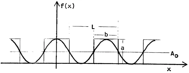
and so on.

Figure

5.

Transmission

Distribution

of a

Symmetrical

[image:18.571.115.485.495.638.2]

11

For

the square wave

in

figure

5,

the real

form

of the

Fourier

series

is:

Ar>

,v

f(x)

= +

J>

Ancos(nwQx)

+

Bnsin(nw0x)

(vi

)

2

i n =

I

where:

A0

=

2C0

An

=

Cn

+ Cn* =

2

(real

part of

Cn)

Bn

=

i(cn

-cn*-

= _-2

(imaginary

_part of

Cn)

For

figure

5,

the

Fourier

coefficients are:

cn

=

ab _{./.,.-_} ab

sin(TTnV0b)

.

sin(nVnb)

=

iL.

(vn)

L

L

TTnV0b

sin(TTnV0b)

LTTnV0b

a

1

sin(TinV

b)

_, since

L

=

Tin

Vc

sin(TT

)

_, since

b

=

L

_

V

_o

lln

2

2

2

Fourier

series and transforms

have

been

put to use

in

the electrical and mechanical

engineering

fields

to solve

a

variety

of problems.

Because

of

the

similarities

among

physical

systems,

the principles of

Fourier

mathematics

12

t(x)

Figure

6.

Transmission Distribution

of a

Symmetrical

Square Wave

and

Its

First

Given

a symmetrical square wave

target,

the

MTF

of an

imaging

system can

be

determined

from

the amplitude spectrum

on the

input

target and the amplitude spectrum of the output

image.

The

Fourier

coefficients at each

harmonic,

divided

by

the

level,

will yield a modulation value and

hence,

a

portion of the

data

point.

MTF

(nw0)

Cn'l/

|C0'|

Cn

|

/

|

C0

|

n -

1

,

2,

3*.

(viii

)

The

prime

figures

represent

data

from

the

output amplitude

spectrum while the others refer to the

input.

One

Fourier

analyzed square wave will yield a number

of useful modulation values.

Therefore,

the total number

of

targets,

exposures,

developments,

and microdensitometer

scans required to compute the

MTF

is

reduced

(compared

to

[image:20.571.74.500.64.291.2]

13

The

proposed

ANSI

standard

for

MTF

determination

requires

at

least

thirteen separate exposures.

Using

a square wave

target and

Fourier

analysis,

the

necessary

number of exposures

is

reduced with no

loss

of

information,

since at

least

three

useable

harmonics

are present at each

frequency.

Twenty-one

data

points can

be

obtained

using

the

square

wave

frequencies

in

table

2.

This

set meets the criterion

set

forth

by

the proposed

ANSI

standard.

TABLE

2

Square

Wave

Frequencies

and

Their

Harmonics

square wave

target

frequency

Fundamental

Cl

Third

C3

Fifth

C5

0.5

cycles

/mm

0.5

1.5

2.5

1.0

1.0

3.0

5.0

2.0

2.0

6.0

10.0

2.5

2.5

7-5

12.5

5.0

5.0

15.0

25.0

20.0

20.0

60.0

100.0

25.0

25.0

75.0

125.0

14

EXPERIMENTAL

The

actual

lab

work was

divided

into

two

sections.

The

determination

of

the

MTF

using

the

conventional sinusoidal method and

the

determination

of

the

MTF

via

the

square wave

method.

Work

on

both

parts progressed simultaneously.

MTF

via

the

Conventional

Method

The

sinusoidal

target

used

for

this

determination

was

obtained

from

the

Photographic

Science

department

at

the

Rochester

Institute

of

Technology.

It

consisted of nineteen

different

frequencies

ranging from

O.36

to

41.6

cycles/mm.

TABLE

3

Frequencies

of

Sinusoidal

Target

0.36

cycles/mm

2.90

9.

09

23.87

0.75

3.77

11.96

29.47

1.11

4.48

15.08

36.57

1.50

6.09

17.78

41.60

15

The

target was

imaged

onto

Kodak

Plus-X

film,

using

a

Polaroid

MP-4

copy

stand with a

4x5

Polaroid

Land

camera.

The

target

was

backlit

using

a

Graphic

Lite

D5000

standard

viewer.

To

produce

the

full

range of

frequencies

desired

(approximately

0.5

to

160.0

cycles/mm),

the

sinusoidal target

was

imaged

with a magnification of

1.0

and

0.25.

The

Plus-X

was

then

developed

in

Kodak

D-76

for

6.75

minutes at

68

F

in

a

hard

rubber

tank.

The

resulting

images

were scanned

with the

Ansco

Model

4

Automatic

Recording

Densitometer.

The

traces

were analyzed and

the

MTF

was plotted

from

the

data.

The

maximum

frequency

obtained with

definite

modulation

was

36.36

cycles/mm.

Since

it

was

felt

that

higher

frequencies

should

be

possible,

the

Polaroid

system was suspected of

having

a ooor

quality

lens.

Since

the

lens

board

mounting

system

made

it

difficult

to substitute another

lens,

a Honeywell

Pentax

35mm

SLR

with a

55mm

lens

was substituted

for

the

4x5

Land

camera.

The

sinusoidal target was again

imaged

at

1.0

and

0.25

magnifications onto

Kodak

Plus-X

135

film.

A

through-focus

series was performed at each magnification.

The

exposed

film

was

developed

in

D-76

for

the recommended

time

at 68

F.

The

exposures made at

0.25

magnification were useless

because

of

heavy

streaks and abrasions

running

through

the

film

strip.

However,

the exposures made at

1.0

magnification were accept

16

was

30.73

cycles/mm.

This

value was also

lower

than what

was

reasonably

expected of the system.

The

resolving

power

was measured

in

an effort to

determine

what

factors

could

be

responsible

for

the

low

frequency

response.

A

through-focus

test was performed on the

MP-4

system with

the

Polaroid

4x5

camera

head.

A

USAF

resolving

power target was

imaged

at a

magnification of

1.0

onto

Plus-X

-+

1

-+7

film.

The

resolving

power of the system was

found

to

be

only

301ines/mm.

The

system was then examined

for

sources of

flare

and a mask

was

incorporated

into

the apparatus to prevent

stray

light

from

the

D5000

from affecting

the exposure.

Resolving

power

increased

to

45

lines/mm

with the use of the mask.

Although

this was a

definite

improvement,

it

was still not at a

level

suitable

for

high

frequency

reproduction.

Since

higher

frequencies

appeared to

be

difficult

to

image

with

the

existing

system,

it

was

decided

that

only

the

frequencies

obtained

with the magnification of

1.0

would

be

used

(table

3).

The

sinusoidal target was then

masked,

imaged

onto

Plus-X

film

using

the

Polaroid

4x5

camera

head,

and

developed

in

D-76

for

7

minutes at 68

F.

The

resulting

images

were scanned

on the microdensitometer, the traces

analyzed,

and

the

MTF

17

MTF

via the

Square

Wave

Method

Several

methods of

manufacturing

a suitable target were

investigated.

The

first

method

involved

the

use of two

Ronchi

rulings,

1.97

and

3.94

cycles/mm.

These

rulings were

imaged onto

Kodak

Aerial

Film

Type

2430

using

the

MP-4 stand

with a

Calumet

4x5

view

camera,

at a magnification of

1.0.

The

Polaroid

camera was not available at this

time.

The

film

was processed

in

Kodak

DK-50

for

the recommended time

at

68

F.

The

resulting

images

were mottled and of

extremely

poor quality.

Variations

in

processing

time,

temperature,

and agitation

failed

to

improve

image

quality.

From

the

procedures

conducted,

it

was concluded that the

film

was

defective

due

to poor storage.

Kodak

Contrast

Process

Pan

Film

Type

4155

was substituted

for

the

2430.

The

rulings

were

imaged

again

using

the

Polaroid

4x5

camera

head.

The

..o

film

was processed

in

D-19

at

68

F.

for

5

minutes.

Although

these

images

were of suitable

quality,

it

proved

difficult

and time

consuming

to adjust magnification and exposure

in

order to obtain the eight targets

desired.

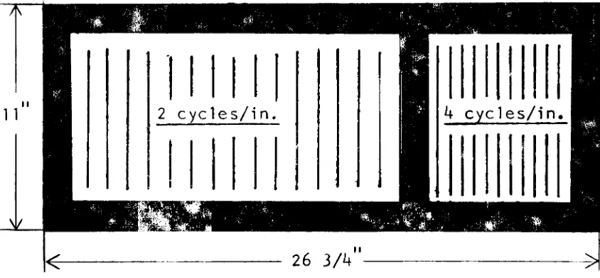
A

second method of

manufacturing

the sauare wave target

involved

the use of Chart-Pak tape affixed to a piece of

white

mounting

board

(Figure

7).

Using

two sizes of

tape,

18

simultaneously.

This

reduced the number of exposures needed

for

the

end product.

The

master was

imaged

onto

General

Photo

Products

lithographic film

at a

3x

reduction

using

a

Kenroe

Vertical

process camera.

The

film

was processed

in

Kodalith

chemistry.

This

system proved _{unsatisfactory}

because

the

maximum

frequency

reproduced was

only

10

cycles/mm.

The

same procedure was then performed

using

a Robertson

Process

camera.

Resoution

increased

to

30

cycles/mm,. It was

decided

to use

this

system to manufacture targets of

0.5,

1.0,

2.0,

2.5,

and

5.0

cycles/mm.

An

additional target wi tha

frequency

of

1.25

cycles.mm was also made.

The

1.0,

1.25,

and

2.0

cydes/mm

targets

were sent to

Photographic

Sciences

Cor

poration where

they

were reduced

20x

to yield targets with

frequencies

of

20,

25,

and

40

cycles/mm.

The

contrast ratio

of the

images

was

approximately

1000:1.

These

eight targets

were then mounted on a glass support to

form

the original

square wave

target.

Since

it

was

desired

to

have

the contrast

ratio of the square wave target equivalent to

the

contrast

of the sinusoidal

target,

the original square wave target

had

to

be

duplicated

onto a

lower

contrast material.

In

order to minimize

harmonic

distortion,

a reversal process

with a gamma of -1 was to

be

used.

The

original square wave

target was contacted onto a sheet of

Rochester

Fi lm

Co.

Type

19

for

5

and

12

minutes

(first

and second

developer,

respec

tively).

Varying

development

times

failed

to

lower

the

gamma

appreciably.

Kodak

Plus-X

type

4147

was then substituted

for

the

3T

microfilm and processed

according

to

an article

2

by

Arthur

S.

Beward

.

Again,

the

gamma was too

high

and

variations

in

processing

failed

to produce significant change,

A

two

step

contact process was substituted

for

the

reversal

system.

The

original square wave target

was

contacted onto

Rochester

Film

Co.

Type

IK

microfilm which was then processed

in

D-19 for

5

minutes at

68

F.

Gamma

of

the

1K

intermediate

was

2.09.

The

IK

intermediate

was

then

contacted to a sheet

of

Kodak

Plus-X

Type

4147.

The

Plus-X

was

developed

in

D-76

for

4

1/2

minutes to yield a

theoretical

gamma of -0.48.

(-0.48)(2.09)

= _-1.00

The

actual gamma

for

the

Plus-X

was-0.42.

Hence,

the

final

gamma

for

the target was-0.88.

This

last

image

is

called

the

final

square wave

target.

Its

contrast ratio

is

approx

imately

10:1.

This

square wave target was then

imaged

onto

Plus-X

type

4147

film

using

the

MP-4

stand with

the

Polaroid

head.

2.

Beward,

Arthur

S.,

"Reversal

Development

of

Black

and

White

Films,"

RIT

Photo

20

A

mask was used with

the

square wave

target

as with

the

sinusoidal

target.

The

exposed

film

was processed

in

D-76

at 68

F.

The

images

were

then

scanned

in

the

microdensi

tometer.

The

traces

were

digitized

and

the

data

entered

into

the

computer.

The

actual calculation of

the

MTF

is

described

in

the

discussion.

[image:28.571.66.488.297.493.2]

21

DISCUSSION

This

section will

begin

with a sample calculation of

an

MTF

value

determined

by

square wave analysis.

Computa

tion of the

sinusoidally

determined

MTF

is

explained

in

the

Theory

section on page

6.

For

this

example,

frequency

patch

#2

(VQ

=

2.011

cydes/mm)

will

be

used.

First,

the

microdensitometer trace

is

examined.

The

frequency

is

calculated

from

a minimum of

10

cycles.

The

maximum and minimum values

for

specular

density

are then noted

for

the same

10

cycles.

They

are then

averaged to yield one maximum and one minimum value.

In

this

case:

Specular

density

Dn*

=

i'i?

Dmin

=

'7

The

next

step

is

to "normalize" the trace to zero.

Thus:

Specular

density

min

=

22

The

specular

density

is

now converted

to

diffuse

density

via

the

equation:

Dd.ff

=

0.751

(Dspec)

+

(3.61

_x

10"3)

=

0.850

Only

the

maximum value

is

used as this represents

the

height

of

the

trace.

The

diffuse

density

is

now converted

to

transmittance.

According

to

the

equation

for

the

real

form

of the

Fourier

coefficients

(equation

vii),

this

will

equal

(a).

transmittance

= _a =

0.143

(xi

)

Substituting

0.143

for

(a)

in

equation

(vii)

yields the

following

values

for

Cn:

Q

Cn

1

0.146

3

0.015

5

0.009

Again,

from

the real

form:

CQ

=

level

=

-2L-=

JL

. since

b

= -~ and

L

=

23

Thus:

C0

=

0.059

From

the

theory,

it

is

shown

that

the

MTF

as

determined

by

the

square wave method of analysis

is

calculated

in

the

following

manner:

ICn'l/lCo'l

MTF

-nwo-jCn

|/|C,

Since

the primed

figures

represent

input

values,

the

denom

inator

refers

to

the

square wave

target.

This

portion

is

calculated

first.

HARMONIC

lnJ/l_Co|

1

0.639

3

0.208

5

0.125

The

next

step

in

the

analysis

is

to

examine

the

micro

densitometer

trace of

the

exposed

images

of

the

square

wave

target

(the

Plus-X

samples).

Again,

10

cycles were

used to calculate the

frequency

of the patch.

Three

cycles

were then chosen at random and specular

densities

read

at equal position

intervals

for

all three.

The

three

readings at each position were averaged

together

to

yield

24

one cycle of

the

square wave at

that

particualr

frequency.

The

computer program utilized

in

this

project was

obtained

from

the

RIT-User's

Computer

Center

library.

It

was written

by

John

R.

Merrill

of

Dartmouth

College.

In

its

original

form,

the

program would generate

its

own set

of

data

as

the

program was

initially

intended

for

instruc

tional

use only.

The

program was modified so

that

any

periodic set of

data

could

be

used.

From

the

data,

the

Fourier

coefficients

(An)

and

(Bn),

and

the

value

(A0)

are computed

(see

equation vi).

An

example of

the

computer

output

for

frequency

patch

#2

is

shown

in

table

4.

TABLE

4

COMPUTER

OUTPUT

SAMPLE

AQ

=

0.774500

HARMONIC

A

B

1

3.90585E-02 -0.366492

3

-2.67930E-03 -4.60720E-02

5

-1.93645E-02 _-2.41352E-03

From

the

derivation

of the real

forms

of

the

Fourier

25

to

(An)

and

(Bn)

in

the

following

manner:

Cnl

= -T-\/An2+

Bn2

UUi)

Sustituting

the

numerical values

from

the

computer output

into

equation

(xi

i i

)

yields:

HARMONIC

[Cn'l

1

0.185

3

0.023

5

0.010

The

numerator of equation

(vi

i

i

)

is

now calculated.

HARMONIC

lcn'l

/I

Co

1

0.477

3

0.119

5

0.026

The

numerator and

denominator

for

equation

(vi

i i

)

have

now

been

computed.

The

actual

MTF

value

is

now calculated,

HARMONIC

MTF

FREQUENCY

1

0.746

1.918

cycles/mm

3

0.570

5.754

5

0.208

9.590

The

MTF

values are then plotted versus

the

corresponding

frequency.

The

total result

is

shown

in

figure

8.

26

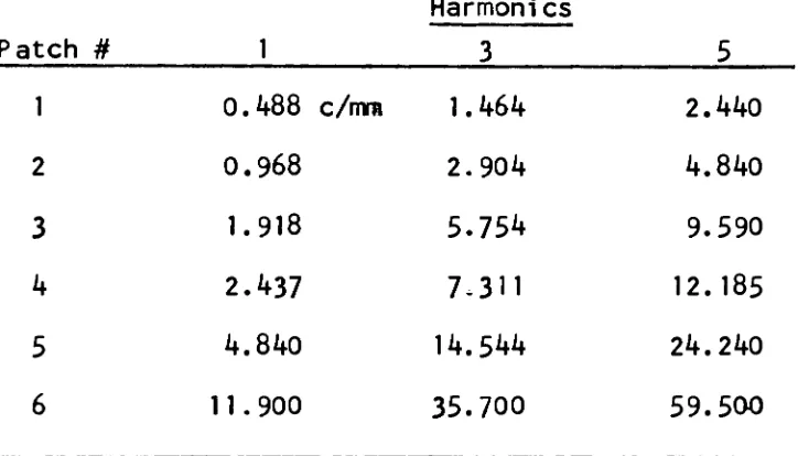
frequencies

of

the

patches on

the

sample.

They

are

directly

proportional to

the

fundamental:

HARMONIC

FREQUENCY

1

x

3

3x

5

5x

TABLE

5

FREQUENCIES

OF

SAMPLE WITH

HARMONICS

Harmonics

Patch

#

1

3

5

1

0.488

ic/mm

1.464

2.440

2

0.968

2.904

4.840

3

1.918

5.754

9.590

4

2.437

7-311

12.185

5

4.840

14.544

24.240

6

1 1

.

900

35.700

59.500

To

simplify

the explanation of the

results,

it

is

initially

assumed that the

MTF

determined

by

the

conventional [image:34.571.105.467.311.518.2]

27

then

be

compared against

this

"correct"

value

for

validity

and accuracy.

The

calculated

MTF's

for

each method of

determination

are plotted

in

Figure

8.

It

can

be

seen that

MTF

measured

by

the

square wave method yielded overall

lower

values

for

the

lower

frequencies

(0

to

9

cydes/mm)

as compared

to

those

values obtained with

the

sinusoidal method.

At

frequencies

higher

than

9

cycles/mm,

the

two

methods yielded

MTF

values

that

were

approximately

equal.

The

dashed

line

is

a plot of

the

MTF

determined

by

the

square wave method

-it has

been drawn

so as

to

smooth

the

trend

of

the

actual

points.

The

solid

line

represents

the

MTF

determined

conventionally.

Both

methods show a peak at

approximately

1.5

cycles/mm,

followed

by

a

decrease

for

frequencies

higher

than

7

cycles/mm.

As

can

be

seen,

there

is

a

large

amount

of

variability

associated with

the

square wave

MTF.

In

addition,

there are two points

(1.464

and

7.311

cycles/mm)

which

fall

in

areas

seemingly

unrelated to

the

general

trend of the graph.

Differences

between

the

output of

the

square wave

method and the conventional method could

be

attributed

to

several possible sources of error.

The

first

of

these

27a

CO TJ O .c jj 0) E

X .* Q>

t/> >

to ro

4-> _{E 3}

ro

SZ XI <u TJ 4J O 1_ Q) j: ro cn ₃ 4J 3 ro cj cr

S c E w r- _O

r- 7 _l W 4- ro

M (J C </)

CU ti o -u

OlTD r-C

1_ 0) 4-> T-ro u c o

h- _{a> a.}

28

target.

When

manufacturing

the

target,

a gamma equal to

-1.0 was required

to

eliminate

harmonic distortion.

The

actual product gamma on

the

square wave target was equal

to-0.88,

thus

indicating

the

inevitable

presence of

dis

tortion,

although minimal.

When

calculating

the

MTF,

harmonic

distortion

was assumed to

be

insignificant to

simplify

calculations.

Related

to

this

are the computations

involving

the

square wave

target

itself.

Examination

of

the

microdensi

tometer

traces

of

the

target showed

that

the

lower

frequencies

(0.5

to

5

cycles/mm) approximated perfect square waves.

The

square wave

target

was therefore assumed perfect so

that

a simplified

formula

for

computing

the

Fourier

coefficients

could

be

used.

This

would then

totally

ignore

the math

ematical considerations

for

any

harmonic

distortion

that

was

present,

not to mention

degradation

of edges and possible

development

effects.

Another

plausible source of error was

the

Ansco

micro

densitometer

used

to

scan the

images.

Once

calibrated,

it

would give reliable readings.

Unfortunately,

due

to

a

drifting

circuit,

re-calibration was required

frequently.

In

addition,

about

midway

through

the

analysis,

repai r work

was performed on

the

instrument.

At

this

time,

the

sinusoid

29

method

MTF

analysis was

just

getting

underway.

Thus,

it

is

possible that

the

adjustments made on the microdensitometer

caused

the

MTF

obtained

by

the

square wave method

to

differ

from

that

of

the

conventionally

determined MTF.

It

is

not conceivable

however,

that

the

microdensitometer was

responsible

for

the

relatively

abnormal

deviations

in

the

MTF

values

for

the

square wave method.

In

doing

the

calculations,

a problem was encountered

when

the

coefficients of

the

target

were compared with the

corresponding

coefficients of

the

sample.

After

the

target

was

made,

it

was scanned with

the

microdensitometer,

and

the

frequency

of each patch calculated.

The

target

was

then

imaged

at a

1.0

magnification onto

Plus-X

film.

This

was

then

scanned,

and

again,

frequencies

were computed

for

each

patch.

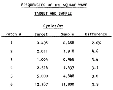
The

target

frequencies

and

the

sample

frequencies,

however,

weren't equal

due

to

a magnification unequal to

exactly

1.0.

The

differences

are shown

in

table

6.

The

frequencies

used

for

figure

8

were the sample

frequencies

-

frequencies

_of

the

harmonics

_{were calculated}

from

these

(see

table

5).

The

equations

for calculating

the

MTF

require

that

the

input

frequency

be

equal to

that

for

the

output

frequency

for

that

specific point.

Although

the

differences

are

slight,

they

could

be

enough to produce

30

[image:39.571.93.465.79.374.2]

TABLE

5

FREQUENCIES

OF THE

SQUARE

WAVE

TARGET

AND

SAMPLE

Cyc1

3s/mm

Patch

#

Target

Sample

Di

fference

1

0.498

0.488

2.0%

2

2.011

1.918

4.6

3

1.004

0.968

3.6

4

2.514

2.437

3.1

5

5.000

4.848

3.0

6

12.387

11.900

3.9

Refering

to

figure

8,

there

are

two

points

(1.464

and

7.311

cycles/mm) on

the

square wave method

MTF

curve which

appear to

bear

no relation to

the

general

trend

of the graph.

Both

these

frequencies

are third

harmonics

derived

from

the

0.488

and

2.437

cycles/mm

frequency

patches respectively.

There

seems to

be

no obvious explanation

for

their

behavior,

as points

derived

from

the

same

frequency

patch

for

the

first

and

fifth

harmonics

follow

the general pattern set

by

the

31

CONCLUSIONS

The

results of

this

research,

specifically

the

com

par

i

si on of the

MTF

as

determined

by

the

two

methods,

can

be

briefly

summarized with

the

following

statements:

1.

There

was more

variability

associated with

the

square wave method of analysis.

2.

Low

frequency

values

(0

to

9

cycles/mm)

generated

with

the

square wave method were

lower

than those

determined

sinusoidally

for

the

same

frequency

range.

3.

High

frequency

values

(9

to

20

cycles/mm)

generated

with the square wave method were

slightly

higher

than

those

obtained

conventionally

over

the

same

range of

frequencies.

4.

Both

methods yielded curves with the same general

trend.

While

it

is

possible

to

name various sources of error

as the causes

for

the

first

three

statements,

the

fourth

clearly

indicates

that

MTF

via a square wave method of

analysis can

be

performed

yielding

results similar

to

a

32

the

shape of the two curves are

relatively

similar suggests

that

the square wave method can

be

used

for

an accurate

MTF

determination.

Elimination

of

the

sources of error

described

in

the

discussion

could

effectively

reduce the

amount of

variability

in

the

square wave

method,

thus

making

it

a reliable measurement.

The

use of a

high quality

square wave

target

in

a

high

resolution photo-optical system

would no

doubt

be

a

first

step

in

reducing

the

variability

encountered

in

this project.

The

results of

this

experiment

are

only

valid,

of

course,

for

the

system that was used.

By

using

Fourier

mathematics,

the square wave

is broken

down

into

sinusoidal components

(harmonics).

The

coefficients

of these

harmonics

are then calculated and

subsequently

used to compute the

MTF.

Thus,

several

data

points can

be

obtained

from

a single square wave

frequency.

In

this

project,

only

the

first,

third,

and

fifth

harmonics

were

used.

Three

points were therefore calculated

from

one

frequency

imaged

on the

film,

thus

reducing

the

number of

required targets

(to

obtain al

1

of the required

frequencies).

In

other

words,

MTF

via square wave analysis

using

a

high

resolution photo-optical system would entail

less

work

than an

MTF

determined

sinusoidally

and yet

it

would retain

33

From

the

outcome of

this

analysis,

it

appears that

the square wave method could

be

a

feasible

route

for

deter

mining

the

MTF

of a photo-optical system.

Although

a

high

degree

of

variability

was encountered

in

the

output of

the

square wave

method,

it

clearly

showed

that

it

followed

the

34

35

o CM O ^O o CN cn c p-P ro o <L> r-> r 1_ a ti ti o a u

r-(T\ r" _{ro o}

M r- _rr\

t/> L. cn r _{a> cm}

i _{u <}

U- <u a;

p c a

u r- _>N

ro ro

36

E * i u-o !_ u 1 2: _ ro (/) 1_ <L> <L) > > 1_ CV ti CXL o

f-o o m

t- 1

+- _CU

m Q.

cn T _>s *rmm _{l_} 1

37

E ^t" ^ 4-O u cj ^ cu z > l_ *: ti . o cu

\ ^~ _o

Q.

\ ^* 1 _>

4-1 I- *

\ . (0

\

-^ r

\

"p~ _{1_ O}

\

u" QJ

38

4-1 M-CU o Di L_ L. u ro r" h- _z: cu *L > ro 12 CU D. CU >N u f-ro _o 3 vO

CT O .

CO o

1-cu E 4-J ^7-ro P" p _Ll. Q CU u E CU i_ 4-1 cu in 4-J _CU c X

11 CJ _o

40

w c cu o

OJ

m

3

0.80

4-1

r~

in

sz CD -a

s_

ro

3 CJ CU

D.

00

0.60

0.40

41

1.00

Fig.

15

Microdensitometer

Calibration

Curve

Sinusoidal

Sample

a.

20

0.40

Diffuse

density

[image:50.571.71.438.148.658.2]

42

4-1

r

in

c cu TJ

CU

m

3

H-

43

>-4-> ^

m

c

QJ TJ

CU

in

3

44

X. m x ro E

\ 4-J _O

SL ro c

,__ _{TJ X}

ro CU 4->

c

cnr-o ro 3

f

E 4- r- _C

c O

cu 4-J

!-> CU -t-i

c cn o

o L_ 3

o ro tj

45

o^ cn -r-.* (/> ro x E u. 0

1 4- _C

2: ro

sz

r _TJ

4-ro <u

c cn 2 0

r _E

c

4-> - _O

c 1

cu M 4->

> CU u

c cn 3

0 U "O 0 fo cu

46

X .*

m u_ ca

1 M E S ro

X

r _TJ 4-J

o ro QJ

T-CM c cn 3 o ro 1

E c U) 4-J r- _O r _c P" Ll. QJ 4-> 4-J

> CU CJ C cn 3 o l_ TJ o ro cu

bl

TABLE

7

PROCESSING

DATA

FOR

FIGURES

8

THROUGH

20

8.

Kodak

Plus-X

Type

4147,

developed

in

D-76

at 68

F

for

7

minutes

9.

Kodak

Fine

Grain Aerial

Duplicating

Film Type

2430,

developed

in

DK-50

for

5

minutes at

68

F*

10.

Rochester

Film

Co.

Type

3T

Reversal

Microfilm,

developed

in

D-19

(2.53

g/1

NaSCN

added)

for

12

and

5

minutes

(1st

and

2nd

developer)

at 68

F

11.

Rochester

Film Co.

Type

IK

Microfilm,

developed

in

D-19

for

5

minutes at 68

F

12.

Rochester

Film

Co.

Type

IK

Microfilm,

developed

in

D-19

for

5

minutes at 68

F

13.

Kodak

Plus-X Type

4147,

developed

in

D-76

for

4

1/2

minutes at 68

F

14.

no

processing

involved

15.

Kodak

Plus-X

Type

4147,

developed

in

D-76

for

7

minutes

at 68

F

16.

Kodak

P

minutes

lus-X

Type

4147,

deveolped

in

D-76

for

4

1/2

, at

686

F

17.

Kodak

Plus-X

Type

4147,

developed

in

D-76

for

7

minutes

at 68

F

18.

Kodak

Plus-X

Type

4147,

developed

in

D-76

for

7

minutes

at 68

F

19,

Kodak

Plus-x Type

4147,

developed

in

D-76

for

7

minutes

at 68

F

20.

Kodak

Plus-X Type

4147,

developed

in

D-76

for

7

minutes

48

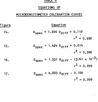
TABLE

8

EQUATIONS

OF

MICRODENSITOMETER

CALIBRATION

CURVES

Figure

Equation

14.

Dspec

=

1.200

Dd.ff

+

0.110

r2

=

0.998

15.

Dspec

=

1.424

Ddiff

+

0.014

r2

=

0.996

.-3-16.

Dspec

=

1.331

Ddiff

-

(3.61

_x

10"J)

r2

=

0.999

17.

DSDec

=0.885

Ddiff

-

0.100

spec

r2

=

0.999

Note:

All

microdensitometer scans were made with a [image:57.571.72.460.117.520.2]

7*9

GENERAL REFERENCES

1.

Kodak

Technical

Pamphlet,

M-61,

Kodak Aerial

Films

and

Photographic Plates

2.

Kodak

Data

Book, P-52,

Techniques

of

Microphotography

Precision

Photography

at

Extended

Reductions

3.

Spiegel, Murray

R.,

Mathematical

Handbook

of

Formulas

and

Tables,

Schaum's

Outline

Series

4.

Sturge,

John

M.

,

editor,

Neblette's

Handbook

of

Photo

graphy

and

Reprography,

Chapter

9,

"The

Microstructure

of

the

Photographic

Image,"

by

M.

Abouelata,

pg

197

5.

Shaw,

Rodney,

editor,

Selected

Readings

in

Image