This is a repository copy of
Tipping Points in 1-dimensional Schelling Models with
Switching Agents
.
White Rose Research Online URL for this paper:
http://eprints.whiterose.ac.uk/90282/
Version: Accepted Version
Article:
Barmpalias, G, Elwes, R and Lewis-Pye, A (2015) Tipping Points in 1-dimensional
Schelling Models with Switching Agents. Journal of Statistical Physics, 158 (4). 806 - 852.
ISSN 0022-4715
https://doi.org/10.1007/s10955-014-1141-5
[email protected] https://eprints.whiterose.ac.uk/
Reuse
Unless indicated otherwise, fulltext items are protected by copyright with all rights reserved. The copyright exception in section 29 of the Copyright, Designs and Patents Act 1988 allows the making of a single copy solely for the purpose of non-commercial research or private study within the limits of fair dealing. The publisher or other rights-holder may allow further reproduction and re-use of this version - refer to the White Rose Research Online record for this item. Where records identify the publisher as the copyright holder, users can verify any specific terms of use on the publisher’s website.
Takedown
If you consider content in White Rose Research Online to be in breach of UK law, please notify us by
(will be inserted by the editor)
Tipping Points in 1-dimensional Schelling Models with Switching
Agents
George Barmpalias · Richard Elwes · Andy Lewis-Pye
Abstract Schelling’s spacial proximity model was an early agent-based model, illustrating how ethnic segregation can emerge, unwanted, from the actions of citizens acting according to individual local prefer-ences. Here a 1-dimensional unperturbed variant is studied under switching agent dynamics, interpretable as beingopen in that agents may enter and exit the model. Following the authors’ work [1] and that of Brandt, Immorlica, Kamath, and Kleinberg in [3], rigorous asymptotic results are established.
The dynamic allows either type to take over almost everywhere. Tipping points are identified between the regions of takeover and staticity. In a generalization of the models considered in [1] and [3], the model’s parameters comprise the initial proportions of the two types, along with independent values of the tolerance for each type.
This model comprises a 1-dimensional spin-1 model with spin dependent external field, as well as providing an example of cascading behaviour within a network.
Keywords Schelling Segregation·Algorithmic Game Theory·Complex Systems·Non-linear Dynamics· Ising model·Spin Glass·Network Science
1 Introduction
The game theorist Thomas Schelling proposed two models of ethnic segregation, which have both proved highly influential as computational/mathematical approaches to understanding social phenomena, as recognised by the Royal Swedish Academy of Sciences on awarding him the Nobel Memorial Prize in 2005 ([20]). In each case, the model comprises a finite number of agents of two types, which we shall take to be green and red. Thespacial proximity orcheckerboard model entails agents taking up positions on a graph or grid (see [22], [23], [25]). Segregated regions may then appear as agents swap to neighbourhoods whose make-up is more to their liking. Subsequently, numerous authors ([26,6,21,8,7]) have observed the structural similarity between this model and variants of the Ising model considered in statistical mechanics for the analysis of phase-transitions. Our model, described in detail in1.1below, will be aSchelling ring, which is to say a 1-dimensional spacial proximity model in which agents take up positions around a circle. We shall follow tradition in framing our discussion in terms of ethnic segregation. However, as has often been remarked, it is equally applicable to any other geographical division of people along binary lines. Examples from [22] include women from men, students from faculty, or officers from enlisted men.
Schelling’s second bounded neighbourhood ortipping model (see [22], [23], [24], [25]) is a non-spacial model, in which a number of agents share a single neighbourhood, and where the initial proportions and preferences of the two types can give rise to total takeover by one type or the other. The simplest case is when no agent wishes to be in the minority, and move out when they are, to be replaced by an agent of the other type. In this case whichever type has more agents initially will take over totally, and thus the tipping point is at the 50% mark. Since Schelling’s insights, tipping points have become a focus of
interest in both the academic literature and popular culture. Models closely related to Schelling’s have subsequently been investigated from a number of angles, notably in the work of Granovetter [12] and as popularised by Gladwell [11].
More immediately, the current paper has its roots in the work of Brandt, Immorlica, Kamath, and Kleinberg [3], which represented a major departure from the numerous previous studies of Schelling segregation, for the first time providing a rigorous mathematical analysis of anunperturbedSchelling ring. Earlier work, notably that of Young [29] and, following him, Zhang ([30], [31], [32]), had concentrated on perturbed models, where agents have a small probability (ε) of acting against their own interests. The introduction of this tiny amount of noise ensures that the resulting Markov process is reversible, and thus considerably easier to analyse. Such models generally exhibit high levels of segregation for anyε >0. Yet it is a well-known principle of statistical physics that perturbed (equivalently non-zero temperature) 1-dimensional models with short-range interactions cannot exhibit phase-transitions. (See [5] for a rigorous modern account of this fact.) It is thus perhaps unsurprising that an unperturbed (ε= 0) model may give rise to profoundly different patterns of segregation from the limiting case (ε→0) of the corresponding perturbed model; the work of [3] established that this does indeed occur, finding dramatically lower levels of segregation in the unperturbed case.
The results of [3] were built upon in [1] by the present authors, which also provided a thorough analysis of an unperturbed Schelling ring, but over a much larger range of parameters. The present model, which we shall describe shortly, continues in the same vein in again providing rigorous mathematical analyses of unperturbed 1-dimensional models, but represents a significant generalization again in terms of their parameters. The major modification relative to [3] and [1] is that we work with an enriched model with the introduction of two additional parameters, which break the symmetry between the two types in two ways. Firstly, we allow the two types to exist in different numbers from one another initially. Secondly the two types may now exhibit unequal levels of tolerance. Both of these are natural extensions of previous models, and indeed were first proposed by Schelling (see for instance [23] p 152).
Another significant difference from the work of [3] and [1] concerns the dynamics by which the model may evolve. Schelling’s original models largely included vacant spaces into which dissatisfied agents could move. Indeed the linear (or 1-dimensional) model described in [23] allows arbitrarily many agents to insert themselves between any two originally adjacent positions. Several subsequent versions of the 1-dimensional model, including those of [3] and [1], have followed Young ([29]) in eliminating vacancies, and instead working with the arguably more realistic “swapping agent” dynamic whereby two unhappy agents of opposite types exchange locations at each time step. Such swapping agent models are thus closed insofar as that the number of agents of each type remains fixed throughout the process, with none entering or leaving.
The primary dynamic we shall work with here is one whereby a single unhappy agent is selected uniformly at random and replaced by one of the opposite type, if doing so will cause the new agent to be happy. We refer to this mechanism as “switching agents”. (We shall also consider two variants of this process described in1.2 below.) Such a dynamic is not new, see for instance recent work of Hazan and Randon-Furling ([13]), who observe that such a set-up has two natural interpretations. Firstly, it can be considered as anopenvariant of the models described in the preceding paragraph, according to which at each time step a single unhappy agent is selected to leave the ring with the resulting vacancy immediately filled by an agent of the opposite type. Thus, as before (and as is perhaps appropriate for a model of ethnic segregation) agents arespatially mobilebutsocially static, that is, the type of each agent remains fixed throughout the process. This open interpretation additionally requires the existence of an unlimited number of agents of both types outside the model who are ready to move in, given the opportunity.
Given these two possible interpretations, we welcome the ambiguity inherent in the phrase “switching agents” as embracing both situations in which agents may switch type, and those where we switch between agents of fixed type.
A deeper remark is that the switching agent dynamic brings the current model closer to the standard spin-1 models of statistical physics (although swapping agent variants also have counterpart in systems employing Kawasaki dynamics). This relationship has been fleshed out elsewhere, especially in [9] where Gauvin, Nadal, and Vannimenus observe that a 2-dimensional open Schelling model is equivalent to a kinetically constrained Blume-Emery-Griffiths spin-1 model. Given this important connection, we spell out in1.3how our model can be recast as a spin-1 model with spin dependent external field.
We wish to mention a final perspective from which one can view the current work, namely in the context of cascading behaviour within networks. A central topic of study in this area is ageneral threshold model. The setting here is a graph, in which every node v is equipped with two things: a function gv
which assigns a valuegv(N) to every subset N of the neighbours of v, and a threshold τv ∈[0,1]. Some
nodes are initiallyactivewhile others are not. At each time stept, every inactive nodevcomputesgv(Atv)
where At
v is the set of neighbours of v which are active at timet. Thenv activates at timet+ 1 if and
only if gv(Atv)≥ τv. The primary question of interest here is to find conditions (on the set of initially
active nodes, the topology of the graph, the functionsgv, and the thresholdsτv) which guarantee that
the whole graph (or most of it) will eventually become activated, or alternatively that the cascade will quickly fizzle out. See [16] for a good survey of this area.
The parallels with the study of Schelling segregation are striking. One major difference, however, is that while general threshold models evolve according to asynchronous dynamic (every agent that may change will do so at each time-step), the literature on Schelling segregation traditionally has one agent (or pair of agents) changing at each time-step. In1.2 below we introduce a synchronous variant of our Schelling model, and see that in many cases (but not all) our conclusions are unaffected by the choice between these dynamics.
Although our model is an instance of Schelling’s spacial proximity model rather than any kind of hybrid or unified model, we nevertheless identify interesting phenomena in the spirit of his tipping or bounded neighbourhood models. That is to say, we shall identify thresholds in parameter-space on one one side of which one type takes over, and on the other side of which the other does. This behaviour is of course only possible in an agent switching model, and furthermore is is only visible from our current asymptotic perspective: we shall prove precise results concerning the ring’s final configuration which are valid as the neighbourhood radius (w) grows large, and the ring size (n) grows large relative tow. More precisely, depending on the initial parameters, one of three conclusions will usually follow in the long run: either the ring will remain essentially static or one type or the other will take over. The asymptotic interpretation is critical here because takeover in this setting need not entail the complete absence of the other type, but rather takeover almost everywhere in a measure-theoretic sense described in1.4 below. Thus takeover or staticity may not be apparent in simulations involving smallwandn. We will identify boundaries between these three regions within the parameter-space of the model.
While the results of [1] were somewhat counterintuitive (and perhaps politically discouraging) in that increased tolerance was seen in certain situations to lead to increased segregation, our results (described in1.6below) on the open model suggest the maxim “tolerance wins out”. Loosely speaking more tolerant groups thrive at the expense of their less tolerant neighbours, although we emphasise that the details are highly sensitive to the initial proportions of the two groups. We also identify two very different regions of staticity, in which very few people move. These occur at the extremes: in one case a ring comprising only very tolerant individuals in which almost everyone is happy with their neighbourhood. We think of this as the region of contentment. In contrast, the region of frustration comprises people so intolerant that, although almost all are unhappy with their neighbourhood, they are also unable to find anyone else prepared to take their place, and thus are forced to stay put.
In more detail, and as already mentioned, our parameters represent a considerable generalisation of those from [1] in two directions. Firstly, we will no longer assume that the initial distribution is symmetric between the two types. Instead, each site will be occupied initially by a green agent with probabilityρ, and by a red agent with probability 1−ρ. Thus it might be that our model describes a homogeneous red region, into which a few green individuals have recently moved (meaning a small value of ρ). It is clearly of interest to be able to predict whether the newcomers will eventually take over the region, or will themselves be squeezed out.
suggested in the past, for example, that black US citizens are happier in integrated neighbourhoods than their white compatriots (see for instance [27]). Thus we introduce two independent parametersτgandτr
representing the tolerance of green and red agents, respectively.
1.1 The model
The model runs as follows. First we fix the parameters n, w ∈ N and ρ, τg, τr ∈ (0,1). The ring then comprises nodes numbered 0 ton−1. We arrange these in a circle, meaning that addresses are computed modnin everything that follows. Initially we populate the ring with agents of two types (red and green), with the colour of each node decided independently according to the toss of a biased coin, each node being green initially with a probability of ρ and red with a probability of 1−ρ. Throughout, a node
x is solely concerned with its neighbourhood of radius w, meaning the w nodes on either side along with itself, amounting to the intervalN(x) = [x−w, x+w] (understood modnas usual). Clearly then |N(x)|= 2w+ 1. Ifxis a green (red) node, it will behappyso long as the proportion of green (red) nodes in this neighbourhood is at least τg(2w+ 1) (respectivelyτr(2w+ 1)), and unhappy otherwise. We say
that an unhappy node ishopeful if a change of colour would cause it to be happy.
(It might be objected that a node’s happiness should depend only on the 2wnodes in its neighbourhood other than itself, rather than incorporating what in neuroscience is termed anautapse, meaning a coupling of the node to itself. However, asymptoticallyC·2w∼C·(2w+1) for allC, and since we will be concerned with behaviour in the large wlimit, the reader interested in the non-autaptic variant of the model will find the main results of this paper unchanged, with only cosmetic modifications of the proofs required. We leave the details as an exercise.)
1.2 The three dynamics
Now we introduce three possible dynamics by which the model may evolve:
• Our primary object of study will be the selective model. Here, at each time-step a hopeful node is selected uniformly at random and its colour changed.
• Theincremental model is similar: at each time-step an unhappy node is selected uniformly at random and its colour changed (regardless of whether this will make it happy).
• In the synchronous model, at each time-step every currently unhappy node alters its colour (again, regardless of the effect on their happiness).
In all cases, the process continues until no further changes are possible, at which stage we say the ring (or process) hasfinished. (We shall establish in Lemma1.19that this is guaranteed to occur for the selective model, and we shall later establish this in certain other cases.) Our principal concern is to find the probability that a randomly selected node is green in the finished ring, and we shall show that this value is usually close to eitherρ, 0, or 1.
1.3 Connections to spin-1 models
Before proceeding to present our results in detail, we pause to recast the discussion above in statistical physical terms. Let us temporarily writeSi(t) = +1 (respectively−1) if nodeiis green (red) at timet.
Then, if nodeiis to update at staget, the procedure by which it does so will be as follows1:
Si(t+ 1) = Sign
X
j:|j−i|≤w Sj(t)
−K(Si(t))
where under the selective dynamic
K(+1) = min{(2τg−1),(1−2τr)} ·(2w+ 1) K(−1) = max{(2τg−1),(1−2τr)} ·(2w+ 1)
1 To be fully correct, we should modify the Sign function such that its behaviour at 0 depends on whetherSi(t) =±1.
and under the incremental and synchronous dynamics
K(+1) = (2τg−1)·(2w+ 1) K(−1) = (1−2τr)·(2w+ 1).
Thus the major difference between our model and a 1-dimensional Ising model with range of interaction
w, is that the termK, which plays the role of the Ising model’s external field, is in our case not uniform across nodes but is instead spin dependent (except in the case τg+τr = 1). As a consequence, if we
attempt to mimic the expression for the Ising model’s energy (suppressing the dependency ont)
H =− X
|i−j|≤w SiSj+
X
i
SiK(Si)
we find that in general it fails to be monotonically decreasing int. For large enoughnandw, the initial configuration is highly likely to contain nodesifor which the value ofP
j:|j−i|≤wSj(t) lie strictly between K(1) andK(−1). Updating such nodes may thus causeH to strictly increase.
In the proof of Lemma 1.19in Appendix A, we nevertheless succeed in developing a harmony index which is monotonic intunder the selective dynamic. We thus hope that the current work can be viewed as a contribution to the study of spin-1 models with spin dependent external field, whose literature does not currently appear especially well-developed.
1.4 A measure-theoretic perspective
As already mentioned, our results are asymptotic in nature. We will use the shorthand “alln≫w≫0” which carries the meaning “all sufficiently largew, and allnsufficiently large relative tow”. By ascenario we mean the class of all rings with fixed values of ρ, τg, and τr, but w andn varying. We will identify
a scenario with its signature triple (ρ, τg, τr), and say that a value ofρadmits scenarios satisfying some
property X, if there exist τg andτr such thatX holds for (ρ, τg, τr). Our conclusions are then of three
types:
• A scenario isstatic almost everywhereif for everyε >0 and alln≫w≫0 a nodexchosen uniformly at random has a probability< εof having changed type at any stage before the ring finishes.
• A scenario suffersgreen (red) takeover almost everywhere if for everyε >0 and alln≫w≫0 a node
xchosen uniformly at random has a probability>1−εof being green (red) in the finished ring.
In some situations we will be able to strengthen the conclusion, and say that green (red)takes over totally if for everyε >0 and alln≫w≫0 the probability that all nodes are green (red) in the finished ring exceeds 1−ε.
1.5 The main thresholds
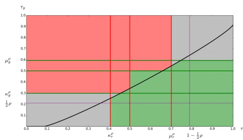
The notions of green/red takeover and staticity almost everywhere divide parameter-space into three main regions. We shall describe tipping points between these in terms of numerical relationships between
ρ,τg, andτr. In particular, for any ρthere exist thresholdsκρg &κρr and µρg= 1−κρr &µρr = 1−κρg as
illustrated in Figure1.
The following give more details:
• Forρ≤1
4 we haveκ
ρ
g< κρr =12 =µ
ρ g< µρr.
• For 14< ρ < 12 we have κρ
g < κρr< 12 < µρg< µρr.
• For ρ = 12 we have κρ
g = κρr ≈ 0.353092313, which is the threshold κ found in [1], and µρg =µρr =
1−κ≈0.64690768667. • For 12< ρ < 34 we have κρ
r < κρg< 12 < µρr< µρg.
• Forρ≥3
4 we haveκ
ρ
r< κρg =12 =µ
ρ κρg κρr
ρ µρg µρr
Fig. 1 The thresholdsκρg &κρrandµρg= 1−κρr &µρr= 1−κρg
As the pair (τg, τr) ranges across the unit square, we shall find that the final configuration of the ring
depends principally on where τg stands in relation to the thresholdsκρg, 12, & µ
ρ
g and where τr stands
regardingκρ
r, 12, & µ
ρ
r, dividing the unit square into up to 16 open regions. We shall be able to analyse
several of these simultaneously, but in some cases we shall find a more delicate dependency between τg
andτr, described shortly. Throughout we shall leave open the intriguing question of what happens when
the parameters exactly coincide with the thresholds. (We remark in passing, that the parameters of the models in [3] and [1] both constitute threshold cases of the current situation.) We shall also leave open the outcomes of the process in two small open regions of the parameter space (see Questions 1.10and
1.14below). We encourage others to investigate these matters.
1.6 Our results
We now state our main results along with some open questions. (These depend on the existence ofκρ g & κρ
r and µρg &µρr described above which will be established rigorously in sections 2 and 6 respectively.)
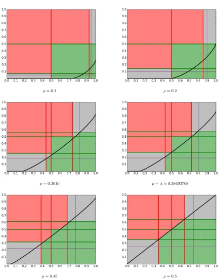
Theorems1.7-1.15which follow are encapsulated (for the casesρ= 0.42 andρ= 0.3) by Figures2and
3. Although the details of the diagrams are specific to ρ= 0.42 and ρ= 0.30, the major features apply more generally. Points coloured grey correspond to scenarios static almost everywhere, while green (red) points indicate green (red) takeover. Purple open regions represent those scenarios, other than those on the thresholds, whose outcome remains unclear. (Notice that there are no such regions in Figure2, which is not unusual. See Questions1.10and1.14.) Similar diagrams for other values ofρare given in Figure4. In each case the roles of red and green may be interchanged by swapping the relevant words, exchanging
ρwith 1−ρ, andκρ
g with κρr, andµρg with µρr. Our first clutch of results (Theorem1.7 -1.11) apply to
all three dynamics, in the situation that at least one ofτg, τr< 12.
Theorem 1.7 Under all three dynamics, if τg< κρg andτr< κρr then the scenario will be static almost
everywhere.
Scenarios whereκρ
r< τr< 12 andτg<12 exhibit a more intricate dependency on (ρ, τg, τr). To resolve
matters here we require the following numerical condition (Definition 3.1 below). A scenario (ρ, τg, τr)
whereρ∈(0,1) andτg, τr∈(0,1) andτg+τr6= 1 is red dominatingif
ρ·
τ
τg 1−τg−τr
g
(1−τg)
1−τg
1−τg−τr <(1−ρ)·
τ
τr 1−τg−τr
r
(1−τr)
1−τr 1−τg−τr .
It isgreen dominating if the reverse strict inequality holds.
Theorem 1.8 Under all three dynamics, if τg< 12 andκρr< τr<12 and(ρ, τg, τr)is green dominating,
then green will take over almost everywhere.
Theorem 1.9 Under all three dynamics, if τg < κρg and κρr < τr< 12, where the scenario is red
[image:7.595.81.493.82.245.2]κρr µρr 1−12ρ
τr
κρg
1 2ρ µρg
τg
Fig. 2 The landscape forρ= 0.42 under the selective dynamic
κρr µρr 1−1
2ρ
τr
κρg
1 2ρ
µρg
τg
Fig. 3 The landscape forρ= 0.3 under the selective dynamic
Open Question 1.10 What is the outcome, under any dynamic, if τg < κρg and κρr < τr < 12, the
scenario is red dominating andτg≤12ρ?
We shall discuss this further at the end of Section 4, but remark that this problematic region only exists for a limited range of values ofρ, namely 14 < ρ < 0.3616 approximately. (Of course exchanging the roles of red and green produces problematic scenarios in the range approximately 0.6384< ρ < 34.)
Notice that the following result has no dependency on ρ:
Theorem 1.11 Under all three dynamics, if τg< 12 < τr green will take over totally.
For the second batch of results (Theorems1.12-1.15), we turn our attention to the case where both
τg, τr> 12. Here, the different dynamics diverge, and our focus will be on the selective case:
[image:8.595.97.485.87.310.2] [image:8.595.115.492.337.563.2]Theorem 1.13 Under the selective dynamic, if 12 < τg < µρg and µρr < τr, where the scenario is red
dominating and additionallyτr<1−12ρ, then the scenario is static almost everywhere.
Open Question 1.14 What is the outcome, under the selective dynamic, of scenarios where12 < τg < µρg
andµρ
r< τr, the scenario is red dominating and τr≥1−12ρ?
The range of ρfor which this mysterious region exists is the same as that for Question1.10above. Our analysis of the selective dynamic culminates in a region of frustration as discussed earlier:
Theorem 1.15 Under the selective dynamic, if µρ
g< τg andµρr< τr, then the scenario is static almost
everywhere.
For the incremental and synchronous dynamics, we shall leave the case τg, τr > 12 largely open.
However, we make the following conjecture:
Conjecture 1.16 Under the incremental and synchronous dynamics, suppose that 12 < τg < τr. Then
green will take over totally. If 1
2 < τg =τr then for any fixed ρthe probability of both red and green total takeover tends to 1 2 as
w, n→ ∞.
Some intuition and partial results towards this conjecture are established in section 8, along with a related discussion of the process’ run-time.
1.17 Interpreting the thresholds
Before we prove Theorems1.7- 1.15rigorously, let us outline the general intuition. Although there will be several technicalities to overcome, the overall strategy is not too complicated and, in the case where
τg<12, amounts to comparing the relative probabilities of unhappy nodes of each colour along with those
ofstable intervals of each colour, in the initial configuration.
The significance of initially unhappy red nodes is that they are likely to spark the growth of green firewalls, which is to say runs of≥w+1 successive green nodes. Whenτg< 12, such a firewall is guaranteed
to grow until it hits astably red interval, meaning an interval of lengthw+ 1 containing enough red nodes (specifically ≥ τr(2w+ 1) many) to ensure that all remain perpetually happy. It is not difficult to see
that stably red intervals stop the growth of green firewalls, and that they are the only things to do so. Given this picture, it is natural that the relative frequencies of stable intervals and unhappy nodes in the initial configuration should be important, and indeed we shall establish that such considerations are decisive. The various thresholds we identify within the regionτg<12 can be understood as follows:
• Forτr> 12, stably red intervals cannot occur for all large enoughw. Thus ifτg< 12< τras in Theorem
1.11, stable green intervals will likely exist in large enough rings (and will serve to prevent total red takeover), as will unhappy nodes of both colours, while stable red intervals will not, suggesting that, eventually, total green takeover cannot be resisted.
• τg =κρg is the point below which stably green intervals become more likely than unhappy green nodes.
Thus if τg < κρg, stably green intervals are more numerous than unhappy green nodes, making red
takeover unlikely.
• Green domination will correspond to unhappy red nodes being more common than unhappy green nodes. Hence, ifτg < 12 and κrρ < τr < 12 hold alongside green domination, as in Theorem1.8, there will be many more unhappy red nodes than green. Since stably red intervals are also infrequent, it follows that many more nodes will be consumed by green firewalls than by red.
Whenτg, τr> 12, under the selective dynamic, similar considerations apply, with a couple of changes:
in the place of unhappy nodes we consider hopeful nodes. (Recall these are unhappy nodes for whom changing colour would produce happiness. This is only automatic, for large enoughw, whenτg+τr<1.)
In the place of stability we considerintractability, which similarly obstructs the growth of firewalls (but cannot occur whenτg, τr<12).
An interval J of length w+ 1 is green intractable if it contains so few green nodes (specifically
< τg(2w+ 1)−(w+ 1) many), that no red node inside J can ever become hopeful, no matter what
• If τg > µρg, then green intractable intervals are more likely than hopeful red nodes, making green
takeover improbable.
• Green domination has an alternative characterisation whenτg, τr>12, as saying that hopeful red nodes
are more likely than hopeful green nodes. If this holds, along with the assumptions that 12 < τg < µρg
and 12 < τras in Theorem1.12, then more green firewalls will start than red ones, and since there are
few green intractable intervals to impede them, we may expect many more nodes to end up green than red.
1.18 Arguing that the ring finishes
As a final step before we launch into an analysis of segregation patterns, we address the question of whether the process is guaranteed to finish. For the selective dynamic, the following result, whose proof is included in AppendixA, is sufficient for our purposes:
Lemma 1.19 For any scenario (ρ, τg, τr)and for all large enough w, the selective dynamic guarantees
that the process will finish.
The observant reader will notice from the proof that the requirement thatwbe large is not necessary in scenarios whereτg, τr<12. Indeed, we expect that it could be dropped in all cases, although this does
not follow from the current argument.
Of course, this implies that a ring under an incremental dynamic and withτg, τr<12 will also finish.
We shall establish certain other cases as consequences of the results in sections5 and 8, however we do not have complete answers for the incremental and synchronous dynamics whenτg, τr > 12. We expect
(indeed it is implicit in Conjecture 1.16) that for any scenario, for any ε >0, and for all large enough
n≫w≫0, the probability that the ring will finish eventually exceeds 1−ε.
2 Stability and Contentment: below the threshold κρ r
We begin with some notation. Given a nodea, we shall writeN(a) := [a−w, a+w] fora’s neighbourhood. Given some collection A of nodes and a timet, we writeGt(A) :=|{x∈A :xis green at timet}|. We
similarly defineRt(A),Ut(A),Ft(A),UGt(A),URt(A),HGt(A),HRt(A),FGt(A) andFRt(A) to be the
number of red, unhappy, hopeful, unhappy green, unhappy red, happy green, happy red nodes, hopeful green, and hopeful red nodes inAat timetrespectively, and will omittwhen its meaning is understood from context. Thus a green node a is happy if G(N(a)) ≥ τg(2w+ 1) and an unhappy red node b is
hopeful if G(N(b))≥ τg(2w+ 1)−1. We will also apply this in the case thatA = {a} is a singleton.
Abusing notation slightly,G(a) can be thought of as the green characteristic function ofa, taking values 0 or 1.
Similarly, an interval [a, a+w] of lengthw+1 isstably greenifG[a, a+w]≥τg(2w+1). We mentioned
in1.17that stably green intervals have the ability to halt the growth of redfirewalls(stretches of at least
w+ 1 consecutive red nodes). We make this precise:
Lemma 2.1 Suppose thatu1 andu2 are nodes such that at timet= 0each ofu1andu2lie in (possibly different) stably green intervals, and there is no unhappy green node in [u1, u2]. Then every green node in[u1, u2]will remain perpetually and happily green.
Proof Suppose not. Then let v in [u1, u2] be the first green node to become unhappy. Now v may only become unhappy once some other green nodev′∈ N(v) has turned red. Sincev′6∈[u1, u2], eitherv′< u1 or v′ > u2. We assume without loss of generality thatv′ < u1. Thenv′ ∈ N(u1). Now by assumption,
u1∈[a, a+w] for some stably green interval [a, a+w]. By stability, we cannot havev′ ∈[a, a+w]. Thus
v′ ∈[u
1−w, a−1], whence it follows that [a, a+w]⊆ N(v) meaning, by stability, thatN(v) contains enough green nodes to keepvhappy, which is a contradiction.
Notice that the possibility of stably green intervals in arbitrarily large rings requires that τg ≤ 12. In
fact we shall assume thatτg < 12 throughout this section, unless stated otherwise. Our goal is to prove
Proposition 2.2 For any ρ∈(0,1), we work in the initial condition, and let Ug be the probability that
a uniformly randomly selected green node is unhappy, and Sg be that of a uniformly randomly selected
node lying within a stably green interval. Then there exists a thresholdκρ
g satisfyingρ > κρg>12ρ, defined as the unique root of the equation
f(s) := 1 2−s
(1−2s)
(1−s)2(1−s) = 1 2(1−ρ).
This is such such that for anyτg∈(0,1):
• If τg< κρg, there existsζ∈(0,1)so that Ug< ζwSg for allw.
• If τg> κρg, there existsζ∈(0,1)so that Sg< ζwUg for allw.
Similarly, there exists a threshold κρ
r where (1−ρ)> κrρ > 12(1−ρ), defined as the unique root of
f(s) =21ρ such that corresponding statements aboutUr andSr hold.
With threshold in place, we shall argue that whenτg< κρg, any randomly selected node is highly likely
be closer on each side to a stably green interval than to an unhappy green node in the initial configura-tion. This will establish that such a node can never turn red, and will be enough to establish Theorem1.7.
Before we proceed with the proof of2.2, we recall two important probabilistic results. The first is a classical result from [14]. (The full statement is more general, but this is the version which shall find most useful.)
Proposition 2.3 (Hoeffding’s inequality) LetX1, . . . , XN be independent random variables such that
P(Xi= 1) =pandP(Xi= 0) = 1−p. Then for any δ >0 we have
P
N
X
i=1
Xi≥(p+δ)N
!
≤exp −2N δ2.
Secondly, we shall require Theorem 1.1 from [2], which appears as Lemma 3.1 in [1], and which we restate:
Lemma 2.4 Suppose h:Z →Z and p∈(0,1) are such that there exist k∈(0,1) so that for all large enough N, we have 1 +1
p−1
kh(N) > N ≥ h(N) > pN > 0. Then for all large enough N, if
XN ∼b(N, p), we have
P(XN =h(N)) ≤ P(XN ≥h(N)) ≤
1 1−k
·P(XN =h(N)).
That is to say in asymptotic notation,P(XN ≥h(N)) = Θ (P(XN =h(N))).
For current purposes, the appropriate asymptotic notion is weaker than Θ:
Remark 2.5 Iff andgare functions ofw, we shall writef ≈gto mean that there are rational functions
P andQsuch that P(w), Q(w)>0 andP(w)g(w)≤f(w)≤Q(w)g(w) for all large enoughw.
Proof (Proof of Proposition2.2)
We fix a scenario (ρ, τg, τr) and work always in the initial configuration. For some green nodeb, we
wish to compare the probability Ug that b is unhappy with the probability Sg that [b−i, b+w−i] is
stably green for someiwhere 0≤i≤w. Our first step is to approximateSgby focusing on the casei= 0.
LetS0
g be the probability that [b, b+w] is stably green. Then Sg ≤(w+ 1)Sg0, meaning that Sg ≈S0g.
We shall therefore work withS0
g in place ofSg, and observe later that this introduces no problems.
Hence the first probability we shall compute is that of the interval [b, b+w] nodes being stably green. Here, the relevant distribution is binomial: X ∼b(w, ρ), describing the number of green elements other thanbin the interval, and Sg≈P(X ≥τg(2w+ 1)−1).
For understanding the likelihood of a green node bbeing unhappy, it will be convenient to count the red nodes inN(b). This is given by the distributionZ ∼b(2w,1−ρ). ThenUg=P(Z >(1−τg)(2w+ 1)).
Remark 2.6 The behaviour of Ug
• If τg≤ ρ2 thenSg≥12 while Ug→0.
• If τg=ρthenSg→0 andUg→ 12.
• If τg> ρ, thenSg→0 andUg→1.
All limits are taken asw→ ∞. Furthermore, it is a straightforward consequence of Hoeffding’s inequality (Proposition 2.3) that the quantities tending to 0 do so at an exponential rate inw, meaning that they are bounded above byνw for someν∈(0,1).
Hence for the remainder of this proof we shall concentrate on scenarios where ρ2 < τg < ρ. We now
apply Lemma2.4in the current context, withN =w,p=ρ, andh(N) =⌈(2w+ 1)τg⌉ −1. Furthermore,
making the assumption thatτg >ρ2 we may findk where 1> k > 1−ρρ ·
1 2−τg
τg . Thus we get
Sg≈ρh(1−ρ)w−h(w)h.
Similarly, assuming only thatτg < ρ, we may take N = 2w,p= 1−ρ, and choosek′ so that 1> k′ >
1−ρ ρ ·
τg
1−τg, to get
Ug≈(1−ρ)h
′
ρ2w−h′( 2 )wh′ (1)
whereh′=⌊(1−τ
g)(2w+ 1)⌋+ 1. Putting these two estimates together, so long as ρ2 < τg< ρ, we find
Ug Sg
≈(1−ρ)h′+h−wρ2w−h′−h( 2 )wh
′
(w) h.
We now employ Stirling’s formula, thatn!≈nn+1
2e−n. Then, the powers ofecancel and we see:
Ug Sg
≈(1−ρ)h′+h−wρ2w−h′−h (2w)
2w+1 2(h)h+
1
2(w−h)w−h+ 1 2
(h′)h′+1
2(2w−h′)2w−h′+ 1 2(w)w+
1 2
. (2)
Now we introduce the approximations 2wτg and 2w(1−τg) for h and h′ respectively. Notice that
|h−2wτg|≤1 and |h′−2w(1−τg)|≤2. It follows easily thathh+
1
2 ≈(2wτ
g)2wτg+
1
2 with ‘≈’ interpreted as in Remark2.5. (We observe in passing that this estimate would not hold under the asymptotic notion Θ.) Similar remarks apply to the other terms in the estimate, allowing us to deduce the following:
Ug Sg
≈(1−ρ)w(2w)2w+
1
2(w(1−2τ
g))w(1−2τg)+
1 2
(2w(1−τg))2w(1−τg)+
1 2(w)w+
1 2
.
Hence we obtain the following key estimate:
Ug Sg
≈ (
1 2−τg)
(1−2τg)
(1−τg)2(1−τg) ·2·(1−ρ) !w
. (3)
The question now is whether the term inside the brackets in3is greater than or less than 1. In many cases there is a threshold,κρ
g, where it is equal to 1. That is,κρg is the root, if it exists, of the equation:
f(s) := 1 2−s
(1−2s)
(1−s)2(1−s) = 1
2(1−ρ). (4)
To establish the existence of this root we shall appeal to the intermediate value theorem, noticing first that for 0< s <12 we have f′(s)>0 meaning that a root, if it exists, will be unique.
We have required that ρ2 < τg< ρandτg< 12. Now we claim the following:
(i) For 0< ρ < 1
2, we havef(ρ)> 1 2(1−ρ). (ii) For 0< ρ < 3
4 we have 1
2(1−ρ) > f(
ρ
2).
To prove (i), define g1(ρ) := (1−ρ)f(ρ) = 1 2−ρ 1−ρ
1−2ρ
. We shall show that g1(ρ) > 1
2. Notice that
g1(0) = 12 so it suffices to show that g′
1(ρ) > 0. Taking logarithms and differentiating, we find that
g2(ρ) := gg1(1(′ ρρ)) = 2 ln(1−ρ)−2 ln(12 −ρ)−1−1ρ. Since g1(ρ)>0 it suffices to show thatg2(ρ)>0. Well
g2(0) = 2 ln 2−1>0 and differentiating again establishes thatg′
The proof of (ii) is similar. Defineg3(ρ) := (1−ρ)f ρ2 = 1
2 1−ρ
1−ρ
1−ρ 2
2−ρ
. We’ll show thatg3(ρ)< 1 2 by a similar argument. Notice that g3(0) = 1
2, hence it will suffice to show that g3′(ρ) < 0. Again, we take logarithms and differentiate, getting g4(ρ) := gg′3(3(ρρ)) = ln 2 + ln 1−ρ2
−ln (1−ρ)− 1−1ρ. Again,
g3(ρ)>0 and we shall show g4(ρ)<0. Well, g4(0) = ln 2−1 <0 and again differentiating establishes thatg′
4(ρ)<0.
What is more, for 1 2 ≤ρ <
3
4, it holds that f( 1 2) >
1
2(1−ρ), where we extend by continuity to take
f 1 2
= 2. Along with (i) and (ii), this allows us to apply the intermediate value theorem. Hence for any 0 < ρ < 3
4 the thresholdκ
ρ
g exists. For τg < κρg we will have Sg ≫ Ug for all large
enoughw, while forτg> κρg we will haveUg ≫Sg.
However, for ρ≥ 34, we get f(s)< 2(11−ρ) for all s < 12. Hence in this regionSg ≫Ug, for all large
enough w, whatever the value of τg < 12. On the other hand, forτg > 12 we haveSg = 0< Ug. Thus it
makes sense to setκρ
g :=12 in this case. We can similarly compute κρ
r, simply by replacingτg with τr and 1−ρ byρin the above analysis,
makingκρ
r the root off(s) = 21ρ. By symmetry, we find that for
1
4 < ρ <1 the thresholdκρr exists. But
whenρ≤14, we have thatSr≫Ur for all large enoughwwhatever the value ofτr< 12.
Finally, recall that at the start of the proof we made the approximationSg≈Sg0. Since estimate3is
exponential inw, the asymptotic limits are unaffected by this move, meaning thatκρ
g and κρr represent
exactly the thresholds we seek. Combining these observations with Remark2.6(and the impossibility of stably green intervals whenτg> 12) we have completed the proof of Proposition2.2.
We may now build towards the proof of our first theorem, that a scenario whereτg< κρg andτr< κρr
will be static almost everywhere.
We begin at a node u0 selected uniformly at random. Looking outwards from u0 in both directions, we may encounter unhappy nodes and/or stable intervals of both colours. We need to understand the most likely order in which we will meet these. It seems plausible, by Proposition2.2, that we are more likely to find green stable intervals before unhappy green nodes, and red stable intervals before unhappy red nodes. Establishing this will suffice, as Lemma2.1then guarantees that there can then be no way for the influence of any unhappy node to reachu0, which must therefore remain unchanged.
We restate the following, which is Lemma 3.2 from [1], recalling that “the first node to the left” of some given nodeusatisfying some criterion means the first in the sequenceu, u−1, u−2,· · ·to satisfy the condition.
Lemma 2.7 Let P(u) and Q(u) be events which only depend on the neighbourhood of u in the initial configuration, meaning that if the neighbourhood ofvin the initial configuration is identical that ofu(i.e. for all i ∈ [−w, w],u+i is of the same type as v+i), then P(u) holds if and only if P(v) holds and similarly for Q(u)andQ(v). Suppose also that:
(i) P(P(u))6= 0 andP(Q(u))6= 0.
(ii) For allk, for all sufficiently large wcompared tok,P(P(u))/P(Q(u))> kw.
For anyu, letxu be the first node to the left ofusuch that eitherP(xu)orQ(xu)holds. For anyε >0,
if0≪w≪n then the following occurs with probability>1−εforuchosen uniformly at random:xu is
defined and for no node v in[xu−2w, xu]does Q(v) hold.
An analogous result holds when ‘left’ is replaced by ‘right’.
We can now establish Theorem1.7. We apply Lemma2.7, interpretingP(u) as the event that the node
ulies in a green stable interval andQ(u) as its being green and unhappy, with Proposition2.2providing the necessary probabilistic bounds. This tells us that, for anyε′>0 and all large enoughn≫w≫0, if we pick a nodeu0uniformly at random, then with probability>1−ε′ the nearest stable green intervals tou0will be closer on both sides than the nearest unhappy green nodes. Thus by Lemma2.1,u0, if green will never turn red.
Then we simply repeat the argument with the roles of red an green interchanged, noting that if two events each have probability tending to 1, then so must their conjunction.
3 Unhappiness and Domination
To analyse the case κρr < τr< 12, we need to answer the following question: in the initial configuration,
Definition 3.1 A scenario(ρ, τg, τr)whereτg+τr6= 1 is red dominatingif
ρ·
τ
τg 1−τg−τr
g
(1−τg)
1−τg
1−τg−τr <(1−ρ)·
τ
τr 1−τg−τr
r
(1−τr)
1−τr 1−τg−τr .
It is green dominatingif the reverse strict inequality holds.
Our choice of terminology will be justified below in Propositions 3.4 and 6.3. Firstly, however we establish some facts about domination, deferring the proof until AppendixB:
Lemma 3.2 LetS:= (0,1)×(0,1). We divideS into the two trianglesT1:={(x, y)∈S:x+y <1}and
T2:={(x, y)∈S:x+y >1} and the lineL={(x, y)∈S:x+y= 1}. Also defineS1:= 0,12× 0,12 andS2:= 12,1× 21,1. (Notice thatSi⊂Ti.) Then the following hold:
1. Suppose that (τg, τr),(τg′, τr′)∈Ti and that(ρ, τg, τr)is red dominating. If τg′ ≥τg, andτr≥τr′ then
(ρ, τ′
g, τr′)is red dominating. Conversely, if (ρ, τg′, τr′)is green dominating, so too is(ρ, τg, τr).
2. For i ∈ {1,2}, every scenario where ρ ≤ 1
5 (respectively ρ ≥ 4
5) and (τg, τr) ∈ Si is red (green) dominating.
3. Any value ofρwhere 15 < ρ < 45 admits both red and green dominating scenarios in bothS1 andS2.
In some cases, red domination is easy to determine:
Corollary 3.3 Suppose (ρ, τg, τr) is a scenario where τg+τr 6= 1 and τg ≥ ρ and τr ≤ 1−ρ. Then
(ρ, τg, τr) is red dominating. (Similarly, green domination follows when both of the reverse inequalities
hold.)
Again we defer the proof to Appendix B. The following result justifies our choice of terminology for scenarios whereτg, τr< 12:
Proposition 3.4 Suppose that τg, τr< 21. The scenario (ρ, τg, τr)is red dominating if and only if there
existsη∈(0,1) so that for allwwe have Ur< ηwUg.
The same holds with the roles of red and green interchanged.
Proof Suppose first thatτg≥ρ, then automatically 1−τr≥ρ, so we may apply Corollary3.3to establish
red domination. Also, Ug →1 (ifτg > ρ) orUg → 12 (ifτg =ρ) asn≫w→ ∞. Meanwhile Ur→0 at
an exponential rate inw. Thus the result follows.
By an identical argument, ifτr≥1−ρthen automaticallyτg< ρand the result follows by Corollary
3.3with the roles of red and green exchanged.
This leaves us with the case whereτg< ρandτr<1−ρ. Under the assumption thatτg< ρ, in
Equa-tion1, we derived an asymptotic expression for Ug. Applying Stirling’s formula and the approximation h′≈2w(1−τg) as previously, it follows that
Ug≈(1−ρ)2w(1−τg)ρ2wτg
(2w)2w+1 2
(2w(1−τg))2w(1−τg)+
1 2(2wτ
g)2wτg+
1 2
.
Of course, by interchanging ρwith 1−ρ, as well asτg withτr, under the assumption thatτr<1−ρ
we may form an analogous expression forUr. We may now take the quotient of these two, to find
Ug Ur
≈
(1−τr)1−τr·τrτr
(1−τg)1−τg·τ τg
g
·ρτg+τr−1·(1−ρ)1−τg−τr 2w
. (5)
The term within the bracket is then > 1 (respectively < 1) if and only if (ρ, τg, τr) is red (green)
dominating, thus establishing the result.
Figure4 depicts the boundary between red and green domination for a few values ofρ. Other details are also shown (exactly as in Figure2), in particular green (red) points on the plane represent scenarios which suffer green (red) takeover, while grey points represent static scenarios. Recall from the discussion following 3 that for ρ ≤ 1
4 our zone of current interest κρr < τr < 12 does not exist, with the fate of
each scenario entirely determined by the value ofτr relative to 12 andµρr and of τg relative toκρg and 12. Nevertheless red/green domination still makes sense as a numerical condition.
Forρ > 14, the zoneκρr< τr<12 does exist, and we observe a form of threshold atρ=λ≈0.38493708
where τλ
discuss it here. By definition, λ is such that (12, κλ
g) and (κλr,12) lie exactly on the boundary between red and green domination. The point of it, therefore, is that for τr < 12 and ρ < λ, green domination
automatically implies thatτg< κρg.
However, forλ < ρ≤ 1
2 green dominating scenarios are also admissible within the zoneκρr < τr < 12
and κρ
g < τg < 12. Notice that atρ= 12, the threshold between red and green domination is simply the
lineτg=τr.
It is clear from Figure4, that forρ > 14, red/green domination can play a decisive role in determining the fate of any scenario. We shall now prove this.
4 Close Contests: between the thresholds κρ r and
1 2
We now wish to apply the results of the previous section to understand scenarios where κρ
r < τr < 12.
This automatically requires ρ > 1
4. We shall make both these assumptions throughout this section, and also insist thatτg< 12, since cases whereτg> 12 will be subsumed into Theorem1.11. However some of
our lemmas will have weaker hypotheses which we shall state explicitly for later reuse.
To begin with, we shall deal with scenarios where (ρ, τg, τr) is green dominating, establishing green
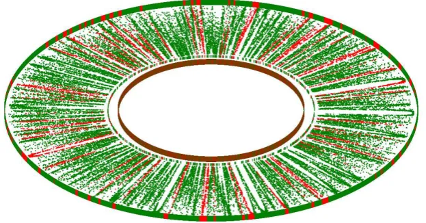
takeover almost everywhere, thus proving Theorem1.8. An example of such a ring is illustrated in Figure
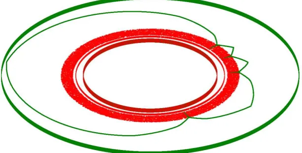
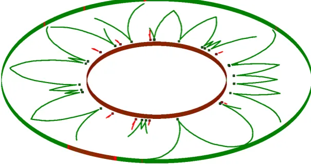
5. (We briefly explain how to interpret such a figure: the initial configuration is shown as the innermost ring, the initially unhappy elements are depicted outside that, and the final configuration is shown in the outermost ring. In between, the elements which change are shown in their new colour, with their distance from the centre proportional to their time of change.)
Our proof will be a modification of Section 4 of [1], and indeed certain things will be simpler in the current case. In outline, the proof will proceed by letting ε > 0 while picking a node u0 uniformly at random, and then seeking to establish that u0 will be green in the final configuration with probability exceeding 1−ε for all n ≫w ≫0. As discussed in1.17, a key notion will be that of a green firewall, meaning a sequence of at least w+ 1 consecutive green nodes. Recall that any firewall is guaranteed to grow in both directions until it hits a stable interval of the opposite colour. Our plan is thus to establish that green firewalls are highly likely to form on both sides ofu0, with no stable red intervals or unhappy green nodes (which may spawn stable red intervals) in positions to block their paths from merging and encompassingu0.
The first step, in Lemma4.7, will be to identify a sequence of nodesli stretching to the left ofu0and
ri to the right. Essentiallyl1 will turn out to be the first node to the left ofu0 whose neighbourhood is such that it will be unhappy if red. Thenl2 will be the first such node to the left ofl1−(2w+ 1), and so on, with theri emerging similarly to the right.
We shall then prove that each of the following statements holds with probability at least 1−ε′ for
arbitraryε′>0, conditional on the previous statements holding. (We withhold the technicalities for now,
including suppressing several intermediate notions.)
• Theliandriexist and satisfy various criteria including the absence of red stable intervals and unhappy
green nodes between them (Lemma4.7).
• The distribution of green nodes in the vicinities of eachli andri issmooth, meaning that there are no
awkward concentrations of red or green nodes nearby. (See Definition4.8and Corollary4.11). • The vicinity of eachli andri is likely to reach maturity without interference from beyond theli orri,
where red firewalls may be growing (Definition4.12and Lemma 4.13). Thus we can be confident that within our region of interest all the changes that occur will consist of red nodes turning green, rather than vice versa.
• Smoothness will then allow us to argue that eachli andri stands a reasonable chance of originating a
green firewall (Corollary4.18and Lemma 4.19).
Together, these will establish that green firewalls are highly likely to grow on both the left and right of u0, and furthermore there will be no red stable intervals in positions to block these firewalls from eventually meeting and consumingu0.
We now begin the proof by recalling some notation from [1] which will be useful when we wish to divide some intervalI intokpieces. The following definition addresses this situation when the length of
ρ= 0.1 ρ= 0.2
ρ= 0.3616 ρ=λ≈0.38493708
ρ= 0.45 ρ= 0.5
Fig. 4 Domination thresholds for various values ofρ. In each caseτr is plotted on the horizontal axis against τg on the vertical. The marked vertical lines represent (in increasing order)κρr, 12,µρr, and 1−12ρ. The horizontal lines are 12ρ,κρg,
1 2, andµ
ρ
[image:16.595.93.527.88.640.2]Fig. 5 ρ= 0.48,τg= 0.38,τr= 0.46,w= 50,n= 100,000, selective dynamic
Definition 4.1 LetI= [a, b]and supposek≥1. We define the subintervalsI(1 :k) :=
a, a+b−a k
:= [I(1 :k)1, I(1 :k)2] and
I(j:k) :=
a+
(j−1)(b−a)
k
+ 1, a+
j(b−a)
k
:= [I(j :k)1, I(j:k)2]
for2≤j≤k.
It will sometimes be useful to count the subintervals from right to left:
Definition 4.2 Let I= [a, b]and suppose k≥1. For 1≤j ≤k we defineI(j :k)− =I(k−j+ 1 :k),
I(j:k)−1 =I(k−j+ 1 :k)1 andI(j:k)−2 =I(k−j+ 1 :k)2.
We now begin to analyse the scenario by picking a nodeu0uniformly at random. The aim of the proof will be to show that for anyε, in the finished ringu0 is green with probability>1−εfor alln≫w≫0. We shall deal separately with the cases 1−ρ≤τr and 1−ρ > τr. We postpone the former situation,
and begin with the case whereγ:= 1−ρ−τr>0. Notice that under this assumption, green domination
implies thatρ > τg via Corollary3.3.
Remark 4.3 There are0< η, ζ <1so that Ug< ηwUr andSr< ζwUr.
This follows from the assumptions of green domination andτr> κρr, by Propositions2.2and3.4.
Remark 4.4 Red nodes are unlikely to be unhappy in the initial configuration:Ur≤exp −2γ2(2w+ 1).
To justify this, letube a randomly selected red node. Then we think ofR0(N(u)) as a sum of 2w+ 1 independent random variables taking the value 1 or 0. Clearly its expected value is (1−ρ)(2w+ 1). Then
Ur=P R0(N(u))< τr(2w+ 1)
=P (1−ρ)(2w+ 1)−R0(N(u))> γ(2w+ 1)
. The remark then follows by Hoeffding’s inequality (Proposition2.3).
Definition 4.5 Letube a node, and letθ∈[0,1]. We sayuhas a local green density ofθor thatGDθ(u)
holds, if G|N0(N(u())u|)) =θ.
We shall be particularly interested in the caseGDθ∗(u) whereθ∗ is as follows:
Definition 4.6 Letθ∗ be minimal such that GD
θ∗(v)implies that v is unhappy if red. That is:
θ∗:= min
m
2w+ 1 :
m
2w+ 1 >1−τr &m∈N
[image:17.595.136.448.95.258.2]Clearly then,θ∗ →1−τ
r as w→ ∞, and it follows from our standing assumption 1−τr−ρ >0 that θ∗> ρfor allw.
Definition of theli andri. We proceed recursively, withl0:=u0. Now defineli+1to be the first node to the left ofli−(2w+ 1) which is either unhappy, or satisfiesGDθ∗, or belongs to a red stable interval, so long as this node lies within [u0−n4]. Theri are defined identically to the right. A little later we shall
choose a specific value ofk0, not depending onw. For now we keep it flexible.
Lemma 4.7 For any k0 >0 and anyε′ >0, there exists d >0 such that for all large enough w andn large enough relative tow, the following hold with probability >1−ε′
1. lk0, . . . , l1, r1, . . . , rk0 are all defined. 2. lk0, . . . , l1, r1, . . . , rk0 all satisfyGDθ∗.
3. There are no unhappy green nodes in[lk0, rk0]. 4. No node in[lk0, rk0]belongs to a stable red interval. 5. Fori≥2, we have|li−1−li|,|ri+1−ri|,|r1−l1|≥edw.
Proof The first four points follow from Remark4.3 and Lemma2.7. The fifth follows from Remark4.4
and the fact that for any intervalI, we haveP(UR(I)>0)≤P
x∈IUR(x).
With all this done, our goal is to show that there is a high chance that at least one of the li and at
least one of theri will originate a green firewall. Since it is very likely that there are no unhappy green
nodes or red stable intervals lying between these nodes, we can then be confident that the two firewalls will merge, thereby encompassingu0. To this end we adapt the following notion from [1]:
Definition 4.8 Suppose thatGDθ(u)holds for someθ. LetL= [u−(3w+1), u]andR= [u, u+(3w+1)].
Suppose that k >0 is a multiple of3 and ε′ >0. Forj ≤k let Rj =R(j :k) andLj =L(j :k)−. We
additionally say that Smoothk,ε′(u)holds if:
• For0≤j≤ k
3, we have
|G0(Lj)|
|Lj| ,
|G0(Rj)|
|Rj| ∈[θ−ε
′, θ+ε′]
• For k3 < j≤k, we have |G0(Lj)|
|Lj| ,
|G0(Rj)|
|Rj| ∈[ρ−ε
′, ρ+ε′]
Thus Smoothk,ε′(u) asserts that the proportion of green nodes inN(v) smoothly moves from θ to ρ
asv moves fromuto u±(2w+ 1).
Corollary 4.9 We make no assumption on (ρ, τg, τr) orθ. For all multiples of threek >0 andε′ >0,
and for all sufficiently large w,
P(Smoothk,ε′(u)|GDθ(u))>1−ε′.
Proof Select uuniformly at random from nodes such thatGDθ(u) holds. We prove the first smoothness
criterion first. The nodes in N(u) form a hypergeometric distribution. Since we consider fixed k andε′
and takewlarge, it suffices to prove the result for givenj with 1≤j ≤k
3. Here the result follows from an application of Chebyshev’s inequality and standard results for the mean and variance of a hypergeometric distribution:
P
G(Lj)
|Lj|
−θ
> ε
′
<|Lj|−2ε′−2 Var(G(Lj)) =O(1)|Lj|−1.
Noting that
|Lj|−(3w+ 1)/k
≤1, the result follows.
Now letu−1=u−(2w+ 1) andu1=u+ (2w+ 1). The fact thatGDθ(u) holds has no impact on the
distributions forN(u−1) and N(u1), where both E(G(N(u1))) =E(G(N(u−1))) =ρ. Thus the second
smoothness criterion follows directly from the weak law of large numbers.
Of course, the li and ri are not selected randomly, so we may not simply apply Corollary 4.9 to
establish their smoothness. Nevertheless we shall be able to deduce it from the following result whose somewhat technical proof is contained in AppendixC:
Proposition 4.10 Fix a value ofρand a valueθ6=ρ. For any node uletxu be the first node to the left
of usuch that GDθ(xu)holds.
Suppose there exists p >0 such that for all sufficiently large w we haveP(Q(u)|GDθ(u))≥p. Then
there exists p′ > 0 such that for all n ≫ w ≫ 0 we have P(Q(xu)) ≥ p′ for u selected uniformly at
random.
If additionally the hypothesis holds with p= 1−ε′ for allε′>0, then we may likewise takep′= 1−ε0 for any ε0>0.
We shall appeal to Proposition 4.10several times, starting with this:
Corollary 4.11 Let ε′>0 andk >0 be a multiple of 3and letk0>0 be fixed. Then for all sufficiently large n ≫w ≫0, with probability >1−ε′ we have that Smoothk,ε′(li) and Smoothk,ε′(ri) hold for all i≤k0.
Proof Corollary 4.9 and Proposition 4.10 combine to tell us that for uniformly randomly selected u, we know that Smoothk,ε′(xu) holds with probability > 1−ε′. Applying this to u = u0 directly tells us that Smoothk,ε′(l1) holds with probability >1−ε′. Of course a symmetric argument applies to r1. Proceeding inductively, suppose that we have established the result for li and ri. Then the sequence of
nodes [li−D, li−(w+ 1)], whereD is any quantity which is small compared to n, is independent of
[li−w, ri+w]. Hence we may apply the same argument again takingu=li−(2w+ 1) to deduce that
Smoothk,ε′(li+1) holds with probability>1−ε′. A symmetric argument works forri+1.
Now, the following definition is valid under all three dynamics. Recall that a node is hopeful if it is unhappy but a change of colour would cause it to become happy, and that we denote the number of hopeful, hopeful green, and hopeful red nodes in a set A at time t by Ft(A), FGt(A) and FRt(A)
respectively. (In our current scenario where τh, τr < 12 hopefulness is automatic for unhappy nodes.
However we shall reuse this notion later in another context.)
Definition 4.12 We say that a nodeugreen completes at stage sif
• Fs(N(u)) = 0, butFt(N(u))>0 for allt < s
• FGt(N(u)) = 0for allt≤s.
For the nodes we consider, it will typically be the case thatFR0(N(u))>0, otherwise we may have the trivial situation of green completion at stage 0.
If ugreen completes it follows thatGt(N(u)) is a monotonic increasing function fort≤s. We shall
apply the following Lemma toli andriwherei < k0, but phrase it more generally for reuse later. Again
the most useful case will be whenuitself is a hopeful red node.
Lemma 4.13 Suppose thatuis a node and thatvandv′are its nearest hopeful green nodes to the left and right respectively in the initial configuration. Assume that there existsd >0so that|u−v|,|v′−u|> ewdfor
allw≫0. Then the following holds independently of all other facts about the ring’s initial configuration: in the selective model with anyτg, τr or in the incremental model withτg, τr< 12, for anyε′>0we have
that u green completes with probability > 1−ε′ for all large enough w. In the synchronous model for
τg, τr< 12 we have instead thatugreen completes with probability1.
Proof We work with the selective/incremental model first. Let I1 = [v, u] andI2 = [u, v′]. Letk be the greatest such that, when 1≤ j ≤ k, I1(j : k) and I2(j : k) are of length ≥w+ 1. For 1 ≤j ≤ ⌊k/2⌋ define:
Jj :=I1(j:k)∪I2(j:k)−.
For 1≤j≤ ⌊k/2⌋, letPj be the event thatR(Jj) increases by 1, and note that Pj+1 cannot occur until
Pjhas occurred. Now the basic idea is that if green completion fails to occur, then the sequence of events P2, ..., P⌊k/2⌋ must occur before any stage whenF(N(u)) = 0.
We label certain stages as being a ‘step towards green completion’, and certain others as being a ‘step towards failure of green completion’.
Steps towards green completion. IfF(N(u))>0 we label any stage at which a node inN(u) changes from red to green as astep towards green completion. OnceF(N(u)) = 0, we consider every step to be a step towards green completion.
Steps towards failure of green completion. If 1≤j <⌊k/2⌋is the greatest such thatPjhas occurred
towards failure of green completion.
We now adopt a modified stage count which counts only steps towards either green completion or its failure. (OnceF(N(u)) = 0, every stage is counted.) Now at any stagesat which somePj forj≤ ⌊k/2⌋
is yet to occur, and at which F(N(u))> 0, the probability of s being a step towards failure of green completion is at most 2(w+ 2) times the probability of it being a step towards green completion (since there are at most 2(w+2) times as many nodes which, if chosen to change, will cause a step towards failure of green completion, as those which will cause a step towards green completion). Choosing 0< d′< dwe
get that for all sufficiently large w,⌊k/2⌋> ed′w
. We may therefore consider the first ed′w
many stages which are steps either towards green completion or failure of completion and, for large w, consider the probability that at most 2w+ 1 of these are steps towards green completion. By the law of large numbers, this probability tends to 0 asw→ ∞. What is more, by assumption onu, 2w+ 1 many such steps more than suffice for its green completion.
For the synchronous model, we simply have to note that sinceed′w
≫2w+ 1 for large enough w, the influence ofv or v′ cannot be felt in N(u) within the first 2w+ 1 time-steps. Thus green completion is
inevitable.
We shall say that a node u originates a green firewall if u green completes, at which time N(u) contains a run of w+ 1 consecutive green nodes. The final step in the proof is to show that each li and ri originates a green firewall with reasonable probability. We have to do a little more work to establish
this, and again we express things more generally. First we establish something weaker, that a firewall gets started in the following sense:
Definition 4.14 With no assumptions on our scenario, let α∈(0,1). We say that a node u α-sparks if u green completes, and at the moment of completion the interval Kα := [u− ⌊α·w⌋, u+⌊α·w⌋] is
completely green.
Our strategy will be to argue, under suitable conditions on α, that each li and ri has a reasonable
chance of α-sparking, and then to establish that such a spark will guarantee the emergence of a green firewall. First, however, we need to consider a technical matter which will become important:
Lemma 4.15 For any θ, ρ∈(0,1), defineZ(θ, ρ) := 1 +θ3−3θ2+ 3θ2ρ−2θ3ρ. Then
(i) ∂Z∂θ <0
(ii) Ifθ < 12(1 +ρ)thenZ(θ, ρ)>0.
Proof To start with, ∂Z ∂θ = 3θ
2−6θ+ 6θρ−6θ2ρ= 3θ(θ−2 +ρ(2−2θ))<3θ(θ−2 + 2−2θ) =−6θ2<0,
establishing the first statement of the lemma for anyθ∈(0,1).
For the second, then, by assumption onθ, we only need to check that
Z
1
2(1 +ρ), ρ
= 3 8−
5 8ρ+
3 8ρ
2+1 8ρ
3−1 4ρ
4>0
which the reader may verify does indeed hold forρ∈(0,1).
Remark 4.16 Lemma4.15 establishes in particular thatZ(θ∗, ρ)>0 for all large enoughw.
To see why the remark holds, recall that the hypotheses of Theorem1.8include the assumption that
τr> κρr and we saw in Proposition2.2, thatκρr>12(1−ρ). Sinceθ∗→1−τr asw→ ∞, it follows that for large enoughw, we shall haveθ∗< 12(1 +ρ).
The following will go most of the way to establishing that theliandrihave a good chance of sparking:
Lemma 4.17 Let Z be as defined in 4.15, and suppose θ is such that Z(θ, ρ) > 0. Suppose that u is uniformly randomly selected from nodes satisfying GDθ(u).
For any α∈ 0,θ
2
, define θα:= θ1−−22αα. Now fix αsmall enough that alsoZ(θα, ρ)>0.
Then there exists δ > 0 (depending on the scenario, θ, and α but not on w) such that if u green completes, then itα-sparks with probability> δ for all w≫0.