Challenges in modelling the random structure correctly in growth mixture models and the impact this has on model mixtures

This is a repository copy of

Challenges in modelling the random structure correctly in

growth mixture models and the impact this has on model mixtures

.

White Rose Research Online URL for this paper:

http://eprints.whiterose.ac.uk/80664/

Version: Published Version

Article:

Gilthorpe, MS, Dahly, DL, Tu, Y-K et al. (2 more authors) (2014) Challenges in modelling

the random structure correctly in growth mixture models and the impact this has on model

mixtures. Journal of Developmental Origins of Health and Disease, 5 (3). 197 - 205. ISSN

2040-1744

https://doi.org/10.1017/S2040174414000130

[email protected] https://eprints.whiterose.ac.uk/

Reuse

Unless indicated otherwise, fulltext items are protected by copyright with all rights reserved. The copyright exception in section 29 of the Copyright, Designs and Patents Act 1988 allows the making of a single copy solely for the purpose of non-commercial research or private study within the limits of fair dealing. The publisher or other rights-holder may allow further reproduction and re-use of this version - refer to the White Rose Research Online record for this item. Where records identify the publisher as the copyright holder, users can verify any specific terms of use on the publisher’s website.

Takedown

If you consider content in White Rose Research Online to be in breach of UK law, please notify us by

Challenges in modelling the random structure correctly in

growth mixture models and the impact this has on model

mixtures

M. S. Gilthorpe1,*, D. L. Dahly2, Y.-K. Tu3, L. D. Kubzansky4and E. Goodman5

1_{Division of Epidemiology & Biostatistics, School of Medicine, University of Leeds, Leeds, UK} 2_{Department of Epidemiology and Public Health, University College Cork, Cork, Ireland}

3_{Institute of Epidemiology & Preventive Medicine, College of Public Health, National Taiwan University, Taipei, Taiwan} 4_{Department of Social and Behavioral Sciences, Harvard School of Public Health, Boston, MA, USA}

5_{Mass General Hospital for Children, Department of Pediatrics, Harvard Medical School, Boston, MA, USA}

Lifecourse trajectories of clinical or anthropological attributes are useful for identifying how our early-life experiences infl_{uence later-life morbidity and}

mortality. Researchers often use growth mixture models (GMMs) to estimate such phenomena. It is common to place constrains on the random part of the GMM to improve parsimony or to aid convergence, but this can lead to an autoregressive structure that distorts the nature of the mixtures and subsequent model interpretation. This is especially true if changes in the outcome within individuals are gradual compared with the magnitude of differences between individuals. This is not widely appreciated, nor is its impact well understood. Using repeat measures of body mass index (BMI) for 1528 US adolescents, we estimated GMMs that required variance–covariance constraints to attain convergence. We contrasted constrained models with and without an autocorrelation structure to assess the impact this had on the ideal number of latent classes, their size and composition. We also contrasted model options using simulations. When the GMM variance–covariance structure was constrained, a within-class autocorrelation structure emerged. When not modelled explicitly, this led to poorer modelfi_{t and models that differed substantially in the ideal number of latent classes, as well as class size and composition. Failure to}

carefully consider the random structure of data within a GMM framework may lead to erroneous model inferences, especially for outcomes with greater within-person than between-person homogeneity, such as BMI. It is crucial to refl_{ect on the underlying data generation processes when building such models.}

Received 8 January 2013; Revised 26 January 2014; Accepted 30 January 2014; First published online 3 March 2014

Key words:autocorrelation, growth, mixtures, random effects

Background

Lifecourse researchers often estimate growth curves or

‘trajectories’in longitudinal data to understand developmental processes. Multilevel modelling1,2is perhaps the most popular method of growth curve estimation in health research, but other useful methods based on structural equation modelling3 are more commonly used in the social sciences. These include latent growth curve modelling (LGCM)4–7and growth mixture modelling (GMM).8–17 In LGCM, repeated measures of a growth variable (e.g. height) are modelled as a function of a smaller number of latent growth factors (analogous to the random effects of multilevel models) and time-specifi_{c latent errors. The}

latent growth factors and errors are each assumed to be independent and identically normally distributed, and the parameters of this

‘random structure’help describe a mean trajectory in the population and how individuals deviate from that trajectory. GMM can be viewed as an extension of LGCM, where model parameters are allowed to vary across a specifi_{ed number of latent classes.}

In seeking a suitable standard GMM, it is currently common practice to estimate multiple models, specifying a different number of latent classes, and make a decision on which model is‘best’. Individuals are classifi_{ed by estimating their posterior}

probabilities of class membership. When a GMM with 2+

latent classes is a better explanation of the observed data than a single class model, it suggests that the population comprises sub-groups, each with its own underlying developmental process. Sub-group membership is interpreted as an important feature in its own right, related to health outcomes and other important covariates. Selecting the model with the ‘correct’

number of latent classes is central to GMM interpretation, and selection can be heavily infl_{uenced by the method used}

to parameterize the structure of random effects within the model. For example, a common approach is to constrain the growth factor variances of all latent classes to be zero, referred to as latent class growth analysis,18 group-based trajectory modelling19 or semi-parametric growth modelling.20 At the other extreme of model parsimony, one could freely estimate the variances and covariances of the growth factors separately for each latent class. It is also common to specify homoscedastic or heteroscedastic models by constraining or freely estimating the latent error variances across time points and/or classes.

*Address for correspondence: M. S. Gilthorpe, Division of Epidemiology & Biostatistics, School of Medicine, University of Leeds, Worsley Building, Clarendon Way, Leeds, LS2 9 LU, UK.

(Email [email protected])

©_{Cambridge University Press and the International Society for Developmental Origins of Health and Disease 2014. The online version} of this article is published within an Open Access environment subject to the conditions of the Creative Commons Attribution licence http://creativecommons.org/licenses/by/3.0/

O R I G I N A L A R T I C L E

Choices regarding model parameterization should be driven by an understanding of underlying data generation processes, associated theory and the research question at hand. GMM convergence can be diffi_{cult when there are too many freely}

estimated parameters. A common solution is to simplify the model with parameter constraints. Although these constraints might be necessary for model estimation, they may not accurately refl_{ect the underlying growth process, and can thus}

lead to erroneous conclusions. When growth factor variances and covariances are constrained to be zero, autocorrelation among the time-specifi_{c latent errors emerges. This occurs if}

individual growth curves are regularly above or below the class-specifi_{c mean growth curve, which is likely for large parts}

of an individual growth trajectory if outcomes exhibit more between-subject than within-subject heterogeneity (which is the case for most human growth measures). This might be resolved by freely estimating the growth factor variances and covariances; however, as noted above, such free estimation may be impossible because of convergence problems. An alternative, more parsimonious approach is to model explicitly the emergent autocorrelation structure. To date, no study has examined the impact of doing this on the selection and interpretation of GMMs. Our study addresses this gap. We consider the simple approach of imposing an autocorrelation constraint on successive measures.

Body mass index (BMI) is a variable of great interest to researchers in a variety offi_{elds and has been studied previously}

using GMM.8,10,12,14,16 We use a motivating example of exploring lifecourse patterns of BMI in a sample of adolescents. Prior work with this cohort has assessed cardiometabolic risk, psychological distress and weight status.21–23 In our illustration, we use these data to generate GMMs to identify lifecourse patterns of BMI, while considering different model parameterizations. We also simulate BMI growth data for a simple model in the same context to help inform interpretation of thefi_{ndings from the genuine data. We contrast constrained}

models with and without an autocorrelation structure, to reveal the impact this has on the derived model, specifi_{cally the ideal}

number of latent classes, their size and their composition. Simulations inform how constraining a GMM’s random structure can introduce an emergent autocorrelation structure, and how failure to model this explicitly can lead to erroneous models being selected.

Methods

The study data set

This study uses longitudinal data from a cohort study conducted in Cincinnati, OH, US area.21–23Data were drawn from Phase 1 of the Princeton City School District study, which began in the 2001–2002 school year and included students in grades 5–12 at baseline with three further annual waves of data collection. Students were excluded if they were pregnant, received corticosteroid treatment for asthma, had a

disease that would interfere with carbohydrate metabolism (diabetes, cancer, cysticfi_{brosis, acromegaly, Cushing’s disease}

or syndrome, pheochromocytoma, liver or kidney disease) or were participating in a longitudinal study of carbohydrate metabolism. Study visits included a physical exam where height and weight were measured. As the cohort was 95% non-Hispanic black and white, analyses were restricted to these two ethnic groups.

Statistical methods

GMM and data simulation were carried out in Mplus version 724 using maximum likelihood (ML) estimation to identify sub-groups that deviated from the ‘normal’ adolescent BMI trajectory. We modelled cohort trajectories (i.e. students nested within measurement occasions, irrespective of their ages) rather than age-specifi_{c growth trajectories (which would overlook the}

natural cohort clustering), as this accurately refl_{ected the}

structure of the data.

BMI trajectories were taken to be quadratic in (centred) time, requiring three latent growth factors, hereby referred to as the intercept, velocity and acceleration. The intercept was modelled conditional on age at thefi_{rst measurement occasion,}

sex, an age–sex product interaction term and racial/ethnic group. Covariate coeffi_{cients were constrained to be identical to}

ensure that the parameterization of underlying BMI growth curves was identical across classes. Individual trajectory differences inmeanBMI by age, sex, age–sex interaction and racial/ethnic group were thus accommodated, as were the different ages at which students were recruited. The age–sex interaction allowed for mean BMI sex differences to vary according to age, and vice versa, accounting for growth spurt differences. As the underlying age, sex and racial/ethnic differences in mean BMI across the classes throughout adolescence were modelled, ‘residual’ differences amount to individual deviations from the underlying mean. Similarly, velocity and acceleration were conditional on age, allowing for differences inchangein BMI by age throughout adolescence. Age and sex differences in BMI changes were captured via the age–sex interaction for the intercept. As initial investigation for age and sex interactions with race revealed small, non-signifi_{cant coef}fi_{cients, differences in BMI changes by}

racial/ethnic group were not modelled. As outcome variances appeared consistent over time, measurement occasion-specifi_c

variances were constrained to be identical across waves within each class (i.e. homoscedasticity was assumed).

Models of the illustrative data with freely estimated variance–covariance structures (i.e. random intercept, velocity and acceleration for each class trajectory) often gave rise to a non-positive defi_{nite covariance matrix, which led to}

diffi_{culties in convergence. This is not unusual with such}

Details of the model specifi_{cation for the illustrative data set are}

given in the Supplementary material.

Model-fi_{t criteria examined were:−2 log-likelihood (−2LL);}

the Akaike’s Information Criterion (AIC=₋2LL₊2k, where

k is the number of model parameters); and the Bayesian Information Criterion (BIC =₋2LL₊k_×ln[n], where k is

the number of model parameters andnis the sample size). The

−2LL improves asymptotically towards model saturation with

increasing model complexity, whereas the inclusion of penalty terms in AIC and BIC attenuate this, both seeking parsimony. Consequently, AIC and BIC can attain minima for relatively low values ofk. Either AIC or BIC may be preferred in pur-suing model parsimony, but one must remain mindful of the impact of parameterization on the utility and meaning of the GMM adopted.

Selection of the‘ideal’number of latent classes should be a combination of likelihood-based model-fi_{t criteria and}

interpretational value. The number of latent classes that we examined for the illustrative data set ranged from 2 to 11. As the risk of models converging to local minima increases with increasing number of classes,25 models were run for 20k random starts (for a limited number of iterations), of which the best 10% (according to ranked LL) were run to completion to derivefi_{nal model estimates; the number of converged models}

was examined to determine what proportion settled on the same ML value.

To evaluate whether models that differed only with regard to the parameterization of autocorrelation had the same individuals allocated to classes, we ranked classes by size for each model type and assessed class‘correspondence’for modal assignment. We used the Rand statistic for cross-classifi_cation

agreement,26 the adjusted Rand statistic which accounts for chance,27 Stuart’s test for homogeneity,28 and a summary measure of net drift of the class membership from larger to smaller classes between models with and without AR1 structure.

Means of residual variances within each class were calculated for all models, weighted according to class size, yielding a measure of within-class random intercept heterogeneity. The overall BMI trajectory intercept variance (constrained to be identical across all classes) provides a measure of between-class random intercept heterogeneity. Both measures refl_{ect how the}

random structure is partitioned within and between classes for each parameterization.

To inform interpretation of thefi_{ndings from the illustrative}

data set, Monte Carlo simulations were undertaken using parameters guided by the genuine data. Details of the model specifi_{cation for the simulated data are given in the online}

appendix. Simulated BMI growth data were evaluated using three GMM parameterizations: (a) unrestricted random effects (refl_{ecting the underlying data generation process);}

(b) restricted random effects comprising random intercept only and no covariance terms (as per the constraints adopted to aid convergence); and (c) identical restricted random effects plus AR1 [a more parsimonious alternative to the unrestricted

random effects that captures the emergent autoregressive (AR) structure]. Models were run for 10k random starts, of which the best 10% were used to derive model estimates. These were summarized over all viable replicates that attained convergence. For parameterizations (b) and (c), models were explored for a number of latent classes to explore changes in model likelihood statistics. Class composition was investigated for a subset of common replicate data sets where convergence was achieved for all parameterizations.

Results

Demographics of the illustrative study in relation to BMI are summarized in Table 1. The cohort was 51.2% female, 47.1% black and had mean age at baseline of 14.4 years (SD= _2.1).

There were no substantive differences by age, sex or ethnicity between the 1528 students who completed two or more study visits (data used for this study) and the 222 who did not (data omitted from this study). All students had BMI assessed at baseline, 78% had a BMI assessment at all four waves, 15% had BMI assessment at three waves and 7% had a BMI assessment at two waves.

A summary of all models explored for the illustrative data, convergence characteristics and model-fi_{t criteria are given in}

Table 2.

Model convergence

Almost all random starts converged for models with no AR1 structure, although the proportion of the best 10% that settled on the same ML value varied, with greater consistency observed for models with two to four latent classes or models with seven and eight classes. Among models with an AR1 structure, only 20% of random starts converged, indicating a limited solution space for models with this random effects parameterization;

Table 1.Study data set structure and features

n(%) Mean BMI (S.D.)

Gender

Male 745 (48.8) 23.0 (5.6)

Female 783 (51.2) 23.7 (6.3)

Race/ethnicity

White 809 (52.9) 22.5 (5.0)

Black 719 (47.1) 24.4 (6.8)

Pubertal status

Puberty 749 (49.1) 21.9 (5.5)

Post-puberty 776 (50.9) 24.8 (6.1)

Parent’s education

<High school 358 (23.4) 23.8 (6.4)

High school 447 (29.3) 24.4 (6.9)

Some college 419 (27.4) 23.0 (5.3)

College or more 304 (19.9) 21.9 (4.3)

that is, many random starts began too far from a viable solution and many more random starts were needed to conduct an exhaustive search for potential solutions. Although one may predetermine starting values, the default is to permit randomly generated initial values. Among the best 10% of models that converged, consistency in the optimum ML varied, but was generally a smaller proportion than for models with no AR1 structure: ML agreement reduced markedly from 100% for the two- and three-class models to 0.2% for the 11-class model.

Likelihood-based model-fit criteria and optimum number of classes

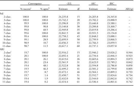
A graphical summary of the likelihood-based model-fi_{t criteria}

is presented in Figure 1. The BIC favoured less complex models over AIC, as anticipated. Models with AR1 consistently

fi_{tted better than those without. For these particular cohort}

data, AIC and BIC never attained a minimum up to the 11 latent classes considered for models without AR1; BIC pla-teaued around 10 or 11 classes. A minimum BIC occurred at six classes for models with AR1.

Class size and composition

Under the null hypothesis of no class discordance between models with or without AR1, class sizes should remain the same and classes ranked by size should correspond to the same class across both model types, with the ideal that class membership corresponds 100%. In practice, although correspondence between models generally decreased smoothly, there were three outlying values for the three-class, six-class and nine-class models when contrasted using modal assignment. The Rand statistic was optimistic, whereas the adjusted Rand, which accommodated chance, suggested modal agreement was often below 50% and near zero for the 3-class, 9-class and 11-class models. For models with three or more classes, there was a netdriftof membership from smaller to larger classes with AR1 incorporated, and this was typically signifi_{cant at the 0.1% level according to Stuart’s test,}

apart from the three-class and seven-class models (Table 3).

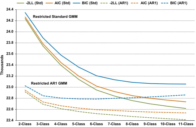
Model random structure

Figure 2 summarizes the weighted mean variation of class

trajectory intercept residual variances and themodeltrajectory Table 2.Summary of growth mixture model (GMM) convergence characteristics and model-fit criteria for the illustrative study data: 10 restricted standard GMMs (Std) and 10 restricted AR1 GMMs (AR1)

Convergence -2LL AIC BIC

% successa % agreeb Estimate df Estimate Estimate AR1(ρ)

Std

2-class 100.0 100.0 24,235.8 15 24,265.8 24,345.8 –

3-class 100.0 100.0 23,742.2 20 23,782.2 23,888.9 –

4-class 99.9 100.0 23,396.8 25 23,446.8 23,580.1 –

5-class 99.8 90.8 23,140.8 30 23,200.8 23,360.7 –

6-class 99.8 60.5 22,949.8 35 23,019.8 23,206.4 –

7-class 99.6 100.0 22,841.5 40 22,921.5 23,134.8 –

8-class 99.4 100.0 22,758.2 45 22,848.2 23,088.1 –

9-class 99.1 28.9 22,699.9 50 22,799.9 23,066.5 –

10-class 98.9 10.7 22,656.3 55 22,766.3 23,059.5 –

11-class 98.7 11.5 22,617.1 60 22,737.1 23,057.0 –

AR1

2-classc 19.7 100.0 22,916.2 15 22,946.2 23,026.2 0.944

3-class 20.1 100.0 22,692.4 21 22,734.4 22,846.3 0.923

4-class 20.1 26.1 22,613.6 26 22,665.6 22,804.3 0.873

5-class 20.1 23.4 22,561.9 31 22,623.9 22,789.2 0.842

6-class 19.4 48.1 22,522.8 36 22,594.8 22,786.8 0.850

7-class 19.5 46.3 22,499.2 41 22,581.2 22,799.8 0.805

8-class 19.7 8.7 22,472.1 46 22,564.1 22,809.3 0.733

9-class 19.7 1.4 22,450.7 51 22,552.7 22,824.6 0.734

10-class 19.4 1.9 22,432.0 56 22,544.0 22,842.6 0.742

11-class 19.4 0.2 22,414.4 61 22,536.4 22,861.6 0.742

LL, log-likelihood; AIC, Akaike’s Information Criterion; BIC, Bayesian Information Criterion; df, degrees of freedom.

a_{Percentage of successes derived as proportion of the 20k random starts that converged to a maximum likelihood.}

b_{Percentage of successes as proportion of the 2k (10%) better models that converged that also agree on the same log-likelihood}

value derived.

intercept residual variance for the range of models considered. Class trajectory intercept residual variances were on average twice of that for models with AR1, indicating that individual trajectories were heterogeneous within classes when autocorrelation was accommodated explicitly. The overall model intercept residual variance was typically a third smaller for models with AR1, revealing that class trajectories were more homogeneousbetweenclasses in models when autocorrelation was accommodated explicitly. This illustrates the extent by which within-model/between-class and within-class trajectories

are affected by the parameterization of the random structure. For these data, the AR1 parameterization elevated random intercept heterogeneity within classes, while reducing random intercept heterogeneity between classes, compared with models with a constrained variance–covariance structure and no

‘compensatory’autocorrelation.

Simulations

Among the simulated data sets, several models failed to converge without a non-positive defi_{nite latent variable covariance matrix,}

indicating either negative variances or residual variances for a latent variable or correlation greater than or equal to one between two latent variables. Modelling complex random structure is thus challenging, which is why constraining random effects to achieve convergence is so appealing. Although each of the one- to three-class restricted random effects models converged easily, this was not true for some of the four- and fi_{ve-class restricted models.}

For the entire range of models considered, there were only nine repeated simulation data sets that were unproblematic for all models (different data sets gave rise to differing convergence problems). Table 4 summarizes the mean likelihood statistics for these data sets.

Under simulation, both the AIC and the BIC favoured the two-class unrestricted model that refl_{ects the underlying}

data generation process. However, when analyses were limited to restricted models (i.e. when unrestricted models fail to converge and more parsimonious random structure is not explored), both the AIC and the BIC favoured models with more than two classes. When random effects were constrained and emergent AR structure modelled explicitly, BIC favoured the correct number of classes, but AIC did not. Likelihood statistics generally favoured models with more classes for the constrained random effects models with no AR1 structure compared with models with AR1.

22.4 22.6 22.8 23.0 23.2 23.4 23.6 23.8 24.0 24.2 24.4

2-Class 3-Class 4-Class 5-Class 6-Class 7-Class 8-Class 9-Class 10-Class 11-Class

Thousands

-2LL (Std) AIC (Std) BIC (Std) -2LL (AR1) AIC (AR1) BIC (AR1)

Restricted Standard GMM

Restricted AR1 GMM

Fig. 1.Likelihood-based model-fi_{t criteria for growth mixture models (GMMs): 10 restricted standard (Std) and 10 restricted AR1 (AR1).}

Table 3. Contrast of class correspondence based on ordered class sizes for 10 growth mixture models (GMMs) with and without AR1 based on modal assignment of 1528 individuals in the illustrative data set

Modal assignment

Classes % correspondence Rand

(%)

Adjusted Rand (%)a

Drift (%)b

2-classc 90.7 83.1 65.9 116

3-class 88.6 50.6 0.3 56

4-class 68.0 77.9 54.1 −175

5-class 66.9 80.3 58.2 −326

6-class 25.1 75.1 34.6 −327

7-class 54.7 80.2 46.3 −320

8-class 45.9 79.6 42.7 −389

9-class 20.5 64.5 −0.6 −214

10-class 40.5 81.6 46.4 −335

11-class 21.3 66.5 0.4 −128

a_{Adjusted Rand accommodates for chance.}

b_{Net difference in the number of individuals within the smaller}

classes within the AR1 model.

c_{For the 2-class AR1 model, the intercept variance was constrained}

When examining class composition via modal assignment there were marked differences (Table 5). Compared with the true generating model, the unrestricted GMM fared well, although it was far from perfect (adjusted Rand was just

>50%). The restricted₊AR1 model did well in recovering

latent class membership and was very similar to the unrestricted GMM. The restricted model without AR1, on the other hand, did considerably worse (adjusted Rand of 0.2%). In contrasting the different parameterizations against each other, the unrestricted and restricted+AR1 models were very similar (class

correspondence>_{90% and adjusted Rand of 72.2%), whereas the}

restricted model with no AR1 was very different from the other two parameterizations in class membership (class correspondence barely over 50% and adjusted Rand<_1%).

Discussion

In lifecourse epidemiology, identifi_{cation of early-life patterns}

or critical periods of growth that might impact health status in later life is a rich and exciting area of research, albeit one fraught with methodological challenges.29 We examine the use of GMMs in the context of lifecourse evaluation of BMI and specifi_{cally re}fl_{ect upon how models are parameterized in terms}

of their random structure. Given the increasing popularity of these methods, it is likely that many applications will adopt constraints for the random structure either as a matter of convenience to promote parsimony or out of necessity to attain model convergence. These constraints will affect the features of interest (i.e. the latent classes), creating the challenge of determining which model parameterization is‘correct’.

Choosing the ‘correct’ model requires an understanding of the context in which data are generated to model variation correctly (i.e. to attain model parsimony without inadvertently imposinginappropriateconstraints). The residual autocorrela-tion between observed values and fi_{tted BMI trajectories is}

often trivial. However, within GMMs, if the variance–

covariance structure is severely restricted, and as BMI exhibits greater within-person than between-person homogeneity (as with most growth measures), residual autocorrelation emerges between individual fi_{tted trajectories and the class}

mean. Methods for modelling an AR structure are varied,30 with one being a simple autocorrelation constraint for successive measures, and another expressing the longitudinal

0.5 1.0 1.5 2.0 2.5 3.0 3.5 4.0 4.5

2-Class 3-Class 4-Class 5-Class 6-Class 7-Class 8-Class 9-Class 10-Class 11-Class

Standard Deviation

Class Residuals (Std) Model Residuals (Std) Class Residuals (AR1) Model Residuals (AR1)

Fig. 2.Variation inclasstrajectory intercept residual variances andmodeltrajectory intercept residual variance: 10 restricted standardgrowth mixture models (GMMs; Std) and 10 restricted AR1 GMMs (AR1); for the two-class AR1 model, intercept variance was constrained to zero to attain convergence with non-negative variances.

Table 4.Mean likelihood statistics for growth mixture models (GMMs) of nine simulated data sets

Mean

-2LL df

Mean AIC

Mean BIC

Mean AR1(ρ)

Unrestricted

2-class 41,877.6 21 41,919.6 42,031.6 –

Restricted standard

1-class 42,130.9 5 42,140.9 42,167.6 –

2-class 41,980.8 11 42,002.8 42,061.5 –

3-class 41,919.5 17 41,953.5 42,044.1 –

4-class 41,892.4 23 41,938.4 42,061.0 –

5-class 41,871.5 29 41,929.5 42,084.2 –

Restricted AR1

1-class 42,017.9 6 42,029.9 42,061.9 0.255

2-class 41,936.9 12 41,960.9 42,024.8 0.269

3-class 41,905.5 18 41,941.5 42,037.4 0.141

variable as an additive function of its immediately preceding values.31An example of the combined attributes of the family of LGCMs, which capture no infl_{uence of the lagged growth}

variable on itself, and the AR models, which do not allow for individual random effects, is the more comprehensive autoregressive latent trajectory (ALT) model.32–34The simple autocorrelation constraint or the ALT model captures the emergent autocorrelation explicitly. For our growth measure, BMI, differences in model fi_{t or overall interpretation from}

either approach are likely to be small, although the exact meaning of model parameters will differ slightly: the AR1 model estimates a correlation coeffi_{cient for successive growth}

measures, whereas the ALT model estimates a regression coeffi_{cient for each growth measure regressed on prior values.}

In both instances, however, the relationship (if any) among the level-1 residuals is confl_{ated with the relationship that}

emerges among trajectory residuals as a consequence of the random effects constraints. Our fi_{ndings suggest that for}

growth measures such as BMI, if the variance–covariance structure is constrained, the emergent AR structure can and should be modelled explicitly, as this leads to model improve-ment and more accurately captures the underlying data generation process.

In practice, selecting the ideal number of classes is informed largely by likelihood statistics but partly by model interpretation. It is clear that parsimony is desirable and the BIC is preferred as it has been shown to perform best of all such information criteria under simulation.35It is also recognized that growth mixtures can be determined in the absence of genuine population hetero-geneity,36 especially if the distribution of growth trajectories is non-normal,37–39 and where covariance misspecifi_{cation is}

restrictive the estimated number of latent classes can be greater than the true number, because more are required to model the extra variability.40For growth data of the kind motivating this

investigation, where BMI is homogeneous over time (near linear), with considerable between-person heterogeneity, where covar-iance constraints are necessary, and there is no clear underlying normal distribution, one has to wonder whether there are any genuine population sub-groups or whether the GMM is merely categorizing a continuum. Given the competing factors that may lead to more classes being determined than are meaningful, it is important to pursue parsimony with GMMs while being careful to capture random structure appropriately. Striking a balance between model complexity in the random structure and parsimony, while not straightforward, is important to determine the correct number and composition of classes if the associated inferences are to be meaningful and robust.

A benefi_{t of modelling the emergent within-class}

autocorrelation to compensate for the variance–covariance constraints is that a larger proportion of individuals are assigned to larger classes compared with models with no autocorrelation structure. Accounting for the random structure effectively homogenizes the larger classes and the LL statistics indicate that modelling autocorrelation in this context provides an improved modelfi_{t; though blindly adopting likelihood-based model-}fi_t

criteria may not always differentiate among plausible models.41 Unsurprisingly, as the number of classes increases, class correspondence decreases between models with and without the AR1 random structure. Class correspondence assumes that

relativeclass sizes remain the same for all models, and hence class ranks remain the same. This is unlikely to hold. For the illustrative data set, the peculiarity of the six-class model in percentage correspondence and the 9-class and 11-class low adjusted Rand statistics were due to diagonals of some class cross-tabulations being zero, suggesting that class correspondence according to ranked class size was inappropriate; with no similar indication for the three-class model, we may only speculate that the assumption was not upheld.

There are a few limitations of this study and its fi_ndings.

First, if the variance–covariance structure of a model must be constrained (e.g. to achieve convergence), the choice of alternative, more parsimonious parameterizations of the random structure is open to evaluation. For instance, the ALT model approach could be considered. We explored a serial correlation term among class trajectory residuals within each growth mixture by incorporating an ARn constraint (withn=_{1, in this instance), and the choice of‘}n_{’is also open}

to evaluation. For both the illustrative and simulated data, there were only four time points and an AR1 was adequate; for more repeated measures a larger‘n’might be warranted. In general, however, we do not propose that a universal alternative approach to modelling random structure in GMMs in the presence of variance–covariance constraints is an AR1 parameterization, as it is advisable to explore a range of model options that are driven by ana prioriunderstanding of the data generation processes. We note, however, that this relatively simple strategy fared well in our study.

Second, although not a problem for our illustrative data, parameterization of a simple polynomial may not always Table 5.Class correspondence for two-class growth mixture models

(GMMs): unrestricted random effects and restricted random effects either with or without AR1: mean (S.D.) modal assignments of 1528 individuals

across the nine simulated data sets

GMM contrast made % correspondence

Rand (%)

Adjusted Rand (%)a

Against true

Unrestricted 86.1 (0.9) 76.1 (1.3) 52.2 (2.5)

Restricted AR1 86.7 (1.2) 76.9 (1.7) 53.8 (3.5)

Restricted 52.2 (1.6) 50.1 (0.1) 0.2 (0.3)

Against each other Unrestrictedv.

restricted AR1

92.5 (1.9) 86.1 (3.2) 72.2 (6.5)

Unrestrictedv.

restricted

52.9 (3.1) 50.3 (0.5) 0.6 (1.1)

Restricted AR1v. restricted

53.3 (2.7) 50.3 (0.5) 0.6 (1.0)

adequately capture the underlying growth trajectories. More sophisticated strategies, such as fractional polynomials splines, or freed-loading models4may be needed.

Third, as often the case in longitudinal epidemiological studies (and in our illustrative data), measurement intervals may not be balanced across individuals, which may lead to inaccuracy in estimating the AR1 structure. We did not adopt a continuous time approach because this caused fewer initial starts to converge, considerably lengthened the time for each model to complete (100-fold), and required imputed ages for missing measurement occasions, without affecting our conclusions (results not shown). In general, however, one should not ignore this added complication. Depending on the data, one solution may be tofi_{t individual curves}fi_{rst, and then}

extract a balanced set of data from those.

Fourth, parameterization of the random variation over time was constrained to be identical for every class. Relaxing this constraint may yield classes that could distinguish between more or less homogeneous individuals (a very plausible scenario), although for the illustrative data set fewer random starts attained convergence and there was no effect to our overall conclusions (results not shown).

Fifth, whether or not the random structure isfi_{xed throughout}

the lifecourse is debatable. BMI generally exhibits greater individual than population homogeneity, but this might vary for different growth periods, such as thefi_{rst few years of life where}

differences between population heterogeneity and individual het-erogeneity are less. Fewer variance–covariance constraints may then be required. Consequently, each stage of the lifecourse must be examined separately for these effects, because implications offi_{ndings on growth throughout adolescence may not generalize}

to other periods of life. The extent of individual and population heterogeneity might vary (i.e. heteroscedasticity), and with variance–covariance constraints the emergent within-class autocorrelation might differ across the different stages of growth. Seeking to accommodate heteroscedasticity throughout different stages of the lifecourse remains an issue for future research.

Finally, it must be recognized that we have undertaken a narrow range of simulations with few parameter specifi_{cations that}

emulate a single observed data set. However, insights gleaned from these simulations clearly demonstrate that tampering with the random structure of GMMs for whatever motive (e.g. parsimony or to aid convergences) has substantive impact on the types of models determined. Our initial fi_{ndings may inform further}

research so that thefi_{eld can advance beyond these limitations.}

Conclusion

Where lifecourse outcomes exhibit greater within-person homogeneity (gradual changes over time) than between-person homogeneity (substantial differences between individuals), and where these outcomes are explored using GMMs with the random effects constrained (for parsimony or to attain convergence), within-class autocorrelation can emerge and should be accommodated explicitly in the model. During puberty,

increased individual heterogeneity is a hallmark of adolescence and is likely to contribute to a reduced degree of within-class autocorrelation owing to greater within-person variation. Adolescence is also a time of elevated between-person hetero-geneity, which is likely to contribute to an increased degree of within-class autocorrelation. The net effect of these two factors is probably population-specifi_{c; however, for our illustrative data,}

substantial within-class autocorrelation was induced once constraints on the random effects were introduced to achieve model convergence. Models with an autocorrelation structure were substantially different from models without yielding different class trajectories with different subjects in each class; these models more likely refl_{ect the underlying data generation processes,}

according to simulations. These fi_{ndings imply that failure}

to model random structure of growth outcomes carefully within a GMM framework can give rise to misleading models and therefore potentially erroneous inferences.

Acknowledgements

Data used in this study were obtained from the Princeton City School District study that was designed and managed by E.G. (any requests for data or associated information should be directed to this author); all analyses were undertaken by M.S. G.; discussion of statistical issues specifi_{cally sought to be}

addressed were led by M.S.G., D.L.D. and Y.K.T., with input and interpretation from E.G. and L.D.K. All authors were responsible for approving thefi_{nal manuscript.}

Financial Support

Funding for the Princeton City School District study data used herein was supported by NIH grants HD041527 and DK59183. DLD was funded by a MRC Population Health Scientist Fellowship, ref: G0902101-1. MSG was part funded by a MRC methodology grant, ref: G1000726.

Confl_{icts of Interest} None.

Ethical Standards

All procedures for the Princeton City School District study were reviewed and approved by the Institutional Review Boards of the participating institutions.

Supplementary Material

To view supplementary material for this article, please visit http://dx.doi.org/10.1017/S2040174414000130.

References

2. Gilthorpe MS, Zamzuri AT, Griffi_{ths GS, Maddick IH, Eaton KA,}

Johnson NW. Unifi_{cation of the‘burst’and‘linear’theories of}

periodontal disease progression: a multilevel manifestation of the same phenomenon.J Dent Res. 2003; 82, 200–205.

3. Kline RB.Principles and Practice of Structural Equation Modeling

2005. Guilford Press: New York.

4. Bollen K, Curran P.Latent Curve Models, 2nd edn, 2006. Wiley: New York.

5. Hjelmborg JB, Fagnani C, Silventoinen K,et al. Genetic infl_{uences on growth traits of BMI: a longitudinal study of}

adult twins.Obesity. 2008; 16, 847–852.

6. Duncan TE, Duncan SE, Stryker LA.An Introduction to Latent Variable Growth Curve Modeling, 2nd edn, 2011. Laurence Erlbaum Associates Inc.: Mahwah, NJ.

7. Harris KM, Perreira KM, Lee D. Obesity in the transition to adulthood: predictions across race/ethnicity, immigrant generation, and sex.Arch Pediatr Adolesc Med. 2009; 163, 1022–1028. 8. Mustillo S, Worthman C, Erkanli A, Keeler G, Angold A,

Costello EJ. Obesity and psychiatric disorder: developmental trajectories.Pediatrics. 2003; 111, 851–859.

9. Bauer DJ, Curran PJ. The integration of continuous and discrete latent variable models: potential problems and promising opportunities.Psychol Methods. 2004; 9, 3–29.

10. Li C, Goran MI, Kaur H, Nollen N, Ahluwalia JS.

Developmental trajectories of overweight during childhood: role of early life factors.Obesity. 2007; 15, 760–771.

11. Kreuter F, Muthen B. Analyzing criminal trajectory profi_les:

bridging multilevel and group-based approaches using growth mixture modeling.J Quant Criminol. 2008; 24, 1–31. 12. Ventura AK, Loken E, Birch LL. Developmental trajectories of

girls’BMI across childhood and adolescence.Obesity. 2009; 17, 2067–2074.

13. deRoon-Cassini TA, Mancini AD, Rusch MD, Bonanno GA. Psychopathology and resilience following traumatic injury: a latent growth mixture model analysis.Rehabil Psychol. 2010; 55, 1–11. 14. Needham BL, Epel ES, Adler NE, Kiefe C. Trajectories of change

in obesity and symptoms of depression: the CARDIA study.Am J Public Health. 2010; 100, 1040–1046.

15. Gentile DA, Choo H, Liau A,et al. Pathological video game use among youths: a two-year longitudinal study.Pediatrics. 2011; 127, e319–e329.

16. Maguen S, Madden E, Cohen B,et al. The relationship between body mass index and mental health among Iraq and Afghanistan veterans.J Gen Intern Med. 2013; 28(Suppl. 2), 563–570. 17. Pickles A, Croudace T. Latent mixture models for multivariate and

longitudinal outcomes.Stat Methods Med Res. 2010; 19, 271–289. 18. Jung T, Wickrama KAS. An introduction to latent class growth

analysis and growth mixture modeling.Soc Personal Psychol Compass. 2008; 2, 302–317.

19. Nagin DS, Odgers CL. Group-based trajectory modeling in clinical research.Ann Rev Clin Psychol. 2010; 6, 109–138. 20. Nagin DS. Analyzing developmental trajectories: a semiparametric,

group-based approach.Psychol Methods. 1999; 4, 139–157. 21. Goodman E, Adler NE, Daniels SR, Morrison JA, Slap GB,

Dolan LM. Impact of objective and subjective social status on obesity in a biracial cohort of adolescents.Obes Res. 2003; 11, 1018–1026.

22. Dolan LM, Bean J, D’Alessio D,et al. Frequency of abnormal carbohydrate metabolism and diabetes in a population-based screening of adolescents.J Pediatr. 2005; 146, 751–758.

23. Kubzansky LD, Gilthorpe MS, Goodman E. A prospective study of psychological distress and weight status in adolescents/ young adults.Ann Behav Med. 2012; 43, 219–228. 24. Muthén LK, Muthén BO.Mplus User’s Guide, 7th edn,

1998–2012. Muthén & Muthén: Los Angeles, CA.

25. Hipp JR, Bauer DJ. Local solutions in the estimation of growth mixture models.Psychol Methods. 2006; 11, 36–53.

26. Rand WM. Objective criteria for the evaluation of clustering methods.J Am Statistical Assoc. 1971; 66, 846–850. 27. Morey LC, Agresti A. The measurement of classifi_cation

agreement: an adjustment to the Rand statistic for chance agreement.Edu Psychol Meas. 1984; 44, 33–37.

28. Stuart A. A test for homogeneity of the marginal distributions in a two-way classifi_{cation.Biometrika. 1955; 42, 412–416.}

29. Tu YK, Tilling K, Sterne JA, Gilthorpe MS. A critical evaluation of statistical approaches to examining the role of growth trajectories in the developmental origins of health and disease.Int J Epidemiol. 2013; 42, 1327–1339.

30. Kessler RC, Greenberg DF.Linear Panel Analysis: Quantitative Models of Change, 1981. Academic Press: New York.

31. Jöreskog KG. A general method for analysis of covariance structures.Biometrika. 1970; 57, 239–251.

32. Curran PJ, Bollen KA. The best of both worlds: combining autoregressive and latent curve models. InMethods for the Analysis of Change(eds. Collins L, Sayer A), 2001; pp. 105–135. American Psychological Association: Washington, DC.

33. McArdle JJ, Hamagami F. Linear dynamic analyses of incomplete longitudinal data. InMethods for the Analysis of Change(eds. Collins L, Sayer A), 2001; pp. 137–176. American Psychological Association: Washington, DC.

34. Bollen KA, Curran PJ. Autoregressive latent trajectory (ALT) models: a synthesis of two traditions.Sociol Methods Res. 2004; 32, 336–383.

35. Nylund KL, Asparoutiov T, Muthen BO. Deciding on the number of classes in latent class analysis and growth mixture modeling: a Monte Carlo simulation study.Struct Equ Modeling. 2007; 14, 535–569.

36. Peugh J, Fan X. How well does growth mixture modeling identify heterogeneous growth trajectories? A simulation study examining GMM’s performance characteristics.Struct Equ Modeling. 2012; 19, 204–226.

37. Bauer DJ, Curran PJ. Distributional assumptions of growth mixture models: implications for overextraction of latent trajectory classes.Psychol Methods. 2003; 8, 338–363.

38. Sterba SK, Mathiowetz RE, Bauer DJ. Adequacy of semiparametric approximations for growth models with nonnormal random effects.

Multivar Behav Res. 2008; 43, 658–659.

39. Van Horn ML, Smith J, Fagan AA,et al. Not quite normal: consequences of violating the assumption of normality in regression mixture models.Struct Equ Modeling. 2012; 19, 227–249.

40. Heggeseth BC, Jewell NP. The impact of covariance

misspecifi_{cation in multivariate Gaussian mixtures on estimation}

and inference: an application to longitudinal modeling.Stat Med. 2013; 32, 2790–2803.

41. Gilthorpe MS, Frydenberg M, Cheng Y, Baelum V. Modeling count data with excessive zeros: the need for class prediction in zero-infl_{ated models and the issue of data generation in}

choosing between zero-infl_{ated and generic mixture models for}

Page | 1

APPENDIX

Model specification for the observed data

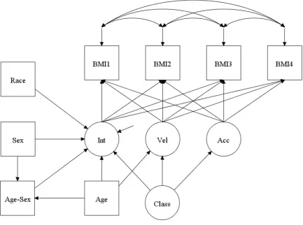
The general form of the growth mixture model for the illustrative dataset was:



















c

ti c ti c

i c

ti i i ti

ti

P

c

age

sex

race

age

age

BMI

2 2 1

0

,

,

|







where

BMI

is an individual's BMI at

age

, measured at time t = 1...4, for individual i =

1...1528; c is the latent class (c = 1...C), for which

P



c

|

age

,

sex

,

race



is the probability

that individual i is in class c given their

age

,

sex

, and

race

;





i ti

c ti c c

ti 0 e0 1age 2sex 3 age sex 4race

0













is the random intercept for class c,

conditioned on age, sex, age-sex interaction and race identically across all C classes;

ti c

c

i 1 5age

1







is the velocity for class c, conditioned on age identically across all C

classes;

0



,

1



, and

2



are the class-dependent marginal mean intercept, velocity and

acceleration respectively;





) ( 0

~

0

,

c

ti

N

e



is the class-dependent occasion-specific normal

residual with zero mean and variance

) (ce0



, estimated empirically; and



(m = 1...5) are

class-independent conditional covariate trajectory coefficients describing the underlying

population mean growth for intercept and velocity respectively. Models were expanded to

include the additional autocorrelation parameter, thereby capturing more of random effects

structure that could not be reflected via the constrained variance-covariance structure. With

only four measurement occasions, we adopted a simple 1

order autoregressive structure

(AR1). For models with AR1 the constraint







(t = 1 ... 3) applies

identically across all C classes, else





(



p



q

). Example M-Plus code

Page | 2

Figure A1: Example M-Plus code for 2-class AR1 GMM with a bootstrapped likelihood ratio test,

for 2000 random starts and 200 fully evaluated starts.

TITLE: Analysis of BMI

DATA:

FILE IS bmi.csv; LISTWISE = OFF;

VARIABLE:

NAMES ARE sch id sex race age1 age2 age3 age4 bmi1 bmi2 bmi3 bmi4

cdc1 cdc2 cdc3 cdc4 wgt1 wgt2 wgt3 wgt4 hgt1 hgt2 hgt3 hgt4

post1 post2 post3 post4 srcesd1 srcesd2 srcesd3 srcesd4

sranx2 sranx3 sranx4 ses1 ses2 ses3 ses4 edu;

MISSING ARE ALL (-99);

USEVARIABLES = sex bmi1-bmi4 race agec agesex sexrace sexm racem agesexm;

AUXILIARY = sex (e) race (e) age1 (e) agesex (e) sexrace (e) cesd1-cesd4 (e)

anx2-anx4 (e) srcesd1-srcesd4 (e) sranx2-sranx4 (e) post1 (e)

ses1-ses4 (e) edu (e);

CLASSES = c(2);

DEFINE:

agec = age1-1.440695; sexm = sex; racem = race; agesexm = agec*sex;

agesex = agec*sex; sexrace = sex*race; ! generated to test only

ANALYSIS:

TYPE = MIXTURE; LRTBOOTSTRAP;

MITERATIONS = 2000; STITERATIONS = 50; PROCESSORS = 8;

MODEL = NOCOVARIANCES;

LRTSTARTS = 2000 200 2000 200;

STARTS = 2000 200;

MODEL:

%OVERALL%

Int Vel Acc | [email protected] [email protected] [email protected] [email protected] ;

Vel-Acc@0;

Int ON agec sexm agesexm racem;

Vel ON agec;

%c#1%

bmi1-bmi4 (resvar1);

bmi1-bmi3 PWITH bmi2-bmi4 (p11);

bmi1-bmi2 PWITH bmi3-bmi4 (p21);

bmi1 WITH bmi4 (p31);

%c#2%

bmi1-bmi4 (resvar2);

bmi1-bmi3 PWITH bmi2-bmi4 (p12);

bmi1-bmi2 PWITH bmi3-bmi4 (p22);

bmi1 WITH bmi4 (p32);

MODEL CONSTRAINT:

NEW (corr);

p11 = resvar1*corr ; p21 = resvar1*corr**2 ; p31 = resvar1*corr**3;

p12 = resvar2*corr ; p22 = resvar2*corr**2 ; p32 = resvar2*corr**3;

OUTPUT:

STAND; TECH14;

SAVEDATA:

FILE = bmi2.dat; SAVE = CPROBABILITIES;

PLOT:

TYPE IS PLOT3;

Page | 3

Figure A2: Model Path Diagram

Model specification for the simulated data

We simulated two BMI latent growth curves following quadratic variation in time.

Fixed-parameter differences were in the BMI mean intercept only and random effects were

different across classes. One hundred replicate datasets were generated, each comprising

1528 individuals at four time points (-1.5, -0.5, 0.5, and 1.5), with BMI mean intercepts 25.0

kg.m

in class 1 and 15.0 kg.m

in class 2; both classes had identical mean velocity (5.0

kg.m

.yr

), mean acceleration (1.0 kg.m

.yr

) and BMI intercept (10.0 kg

.m

.yr

), velocity

(5.0 kg

.m

.yr

) and acceleration (1,0 kg

.m

.yr

) variances. In class 1, the BMI

intercept-velocity covariance was 0.2 (correlation = 0.028) and intercept-acceleration covariance was

0.1 (correlation = 0.032), whereas in class 2 these were -0.2 (correlation = -0.028) and -0.1

(correlation = -0.032), respectively, and for both classes the velocity-acceleration covariance

was 0.05 (correlation = 0.022). The intercept, velocity and acceleration were not dependent

Page | 4

study data exactly, as no attempt was made to simulate emulate ages at each time point or

age-related effects (such as individual growth spurts). This should not affect any inferences

made regarding differences in model parameterization. The simulations broadly capture the

concept of a near linear change in BMI over time, with large heterogeneity between

individuals and small heterogeneity within individuals between measurement occasions, as