Adiabatic quantum optimization
in the presence of discrete noise:
Reducing the problem dimensionality
The Harvard community has made this
article openly available. Please share how
this access benefits you. Your story matters
Citation
Mandrà, Salvatore, Gian Giacomo Guerreschi, and Alán
Aspuru-Guzik. 2015. “Adiabatic Quantum Optimization in the Presence of
Discrete Noise: Reducing the Problem Dimensionality.” Physical
Review A 92 (6) (December 10). doi:10.1103/physreva.92.062320.
Published Version
doi:http://dx.doi.org/10.1103/PhysRevA.92.062320
Citable link
http://nrs.harvard.edu/urn-3:HUL.InstRepos:24873724
dimensionality
Salvatore Mandr`a∗, Gian Giacomo Guerreschi∗, and Al´an Aspuru-Guzik
Department of Chemistry and Chemical Biology, Harvard University, 12 Oxford Street, 02138 Cambridge MA
Adiabatic quantum optimization is a procedure to solve a vast class of optimization problems by slowly changing the Hamiltonian of a quantum system. The evolution time necessary for the algorithm to be successful scales inversely with the minimum energy gap encountered during the dynamics. Unfortunately, the direct calculation of the gap is strongly limited by the exponential growth in the dimensionality of the Hilbert space associated to the quantum system. Although many special-purpose methods have been devised to reduce the effective dimensionality, they are strongly limited to particular classes of problems with evident symmetries. Moreover, little is known about the computational power of adiabatic quantum optimizers in real-world conditions. Here, we propose and implement a general purposes reduction method that does not rely on any explicit symmetry and which requires, under certain general conditions, only a polynomial amount of classical resources. Thanks to this method, we are able to analyze the performance of “non-ideal” quantum adiabatic optimizers to solve the well-known Grover problem, namely the search of target entries in an unsorted database, in the presence of discrete local defects. In this case, we show that adiabatic quantum optimization, even if affected by random noise, is still potentially faster than any classical algorithm.
I. INTRODUCTION
In 2001, Farhi et al. [1] proposed a new paradigm to carry out quantum computation (QC) that is based on the adiabatic evolution of a quantum system under a slowly changing Hamiltonian and that builds on previous results developed by the statistical and chemical physics communities in the context of quantum annealing tech-niques [2–5]. While this approach constitutes an alterna-tive framework in which the development of new quan-tum algorithms for optimization problems results more intuitive [6–8], the estimation of the evolution time and its scaling with the problem size still remains unclear. For example, factors like the choice of the schedule [9, 10] and the specific form of the Hamiltonian [11–14] influence the adiabatic evolution in ways that are, so far, not fully un-derstood. Adiabatic QC at zero temperature has been proved to be polynomially equivalent to the usual QC with gates and circuits [15, 16] and, therefore, any expo-nential quantum speedup should be attainable [17–20]. In this respect, several numerical studies carried out in the last few years reported encouraging results for small systems [1, 14, 21–24], exactly solvable systems [7, 9], and specific quantum chemistry or state preparation prob-lems [25–28]. In contrast, recent results in the context of experimental quantum annealing machines, which oper-ate according to the same principle of adiabatic QC but in a thermal environment, showed no evidence of quan-tum speedup for random optimization problems [29].
To shed light on the actual power of QC, it is of great importance to be able to perform extensive numerical and theoretical studies on large quantum systems. Un-fortunately, these kinds of analyses are strongly limited by the exponential growth in dimensionality of quantum systems. In the context of adiabatic QC, the evolution time, and thus the computational effort it quantifies, is
related to the minimum energy gap between the ground state and the first excited state along the quantum evo-lution. The direct calculation of the energy gap is feasi-ble only for optimization profeasi-blems up ton≈30 qubits [1, 21, 22, 24]. Estimations through quantum Monte Carlo techniques work only at finite temperature and re-quire a large overhead due to the equilibration and evo-lution steps necessary to describe the situation at every stage of the adiabatic process [30–33].
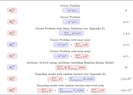
In the past few years, several studies introduced special-purpose techniques to reduce the dimensionality of particular classes of problems that are based on ex-plicit symmetries of the QC Hamiltonian. For example, algorithms involving the Grover-style driver Hamiltonian have been analyzed in the subspace of states symmetric under the exchange of any two qubits [9, 34, 35], while cost functions that depend only on the Hamming weight ofn-bit strings have been solved by reducing the system to an effective single spinn/2 [36]. However, no clear way to extend such approaches to non-symmetric situations has been suggested. Here, we propose and implement a novel method to study large adiabatic quantum optimiz-ers by reducing the dimensionality of their Hilbert spaces. Our approach does not rely on any explicit symmetry and goes beyond the strict distinction of driver and problem contributions to the Hamiltonian (see Table 1).
The development of the present method allows us to perform the exact calculation of the minimum gap for systems outside the usual assumption of an ideal, isolated adiabatic quantum optimizer. In this direction, only few studies on simplified 2-level systems have addressed the effect of thermal noise on adiabatic quantum optimization (AQO) [37]. Here, we apply the dimensionality reduction to the Grover search problem in presence of stochastic local noise (see Table 1), using two common choices of the driver Hamiltonian. We are
Driver Hamiltonian Problem Hamiltonian Dimensionality
Grover Problem
HD(G) − |σ∗ihσ∗| 2
Grover Problem
HD(S) − |σ
∗
ihσ∗| n+1
Grover Problem with Many Solutions (see Appendix E)
HD(S) −Pp
i=1|σ
∗
iihσ
∗
i| ≤p n
Grover Problem with local noise
HD(G) − |σ∗ihσ∗| + Pn i=1iσˆ
z
i n+2
Grover Problem with local noise
HD(S) − |σ∗ihσ∗| + Pn i=1iσˆ
z
i n+1
Arbitrary M-level energy problems (including Random Energy Model)
HD(G) PM
i=1EiPσ∈ωEi|σihσ| M
Tunneling model with random barriers (see Appendix B)
HD(S) −Pn
i=1ˆσ z i +
P
σ|ω(σ)=1Vσ|σihσ| ≤(n+2) 2
Tunneling model with random barriers and local noise
HD(S) −Pn i=1σˆ
z
i + Pσ|ω(σ)=1Vσ|σihσ| +
Pn i=1iσˆ
z
[image:3.612.91.522.66.374.2]i ≤(n+1)3
TABLE I.Examples where the proposed method gives an exponential reduction. Light-shaded boxes (red on-line) and dark-shaded boxes (blue on-on-line) correspond to HA and HB respectively as explained in the main
text.The first column indicates the choice of the driver Hamiltonian corresponding to either the Grover-styleHD(G)=− |ψ0ihψ0|
or the standard oneHD(S)=−Pn i=1ˆσ
x
i. The second column describes the optimization problem and the third column provides
an upper bound on the dimensionality after the reduction method for a system of n qubits (to be compared with the total number of stateN= 2n). The explanation of the symbols is as follows: |σiis the state of the computational basis corresponding to then-bit stringσ∈ {0,1}n
,|ψ0iis the balanced superposition of all the computational basis states,π(·) is a permutation
of{1,2, . . . , n},w(·) the Hamming weight of a bit string, ˆσz
i and ˆσxi are respectively the PauliX and PauliY matrices acting
on thei−th qubit, ΩE is the eigenspace associated with eigenvalueE,i=±||and||, E, Vσ are real coefficients.
able to show that a quantum speedup is retained when an appropriate schedule, independent of the choice of the target state, is implemented. To our knowledge, these are the only conclusive results on the performance of adiabatic QC in presence of local noise that has been reported so far, together with works on the effect of thermal baths [37, 38] and on the specific D-wave hardware [39, 40].
The rest of the article is structured as follows: In Sec-tion II, we introduce the adiabatic quantum optimizaSec-tion and the main relevant quantities. In Section III and Sec-tion IV, we present our method and provide its detailed derivation. The application of our method to the noisy Grover problem is then described in Section V, while in the last Section we provide final discussions and conclu-sions.
II. ADIABATIC QUANTUM OPTIMIZATION
In adiabatic quantum optimization, computational problems can be rephrased in terms of finding those states which minimize a classical cost function encoded by a diagonal Hamiltonian. The adiabatic theorem [41, 42] implies that a quantum system remains in its instantaneous ground state if the quantum Hamiltonian is slowly deformed. Following the above considerations, Farhi et al. [1] proposed to govern the dynamics of a quantum optimizer by a time dependent Hamiltonian of the form:
by the adiabatic schedule s(t) satisfying the boundary conditionss(0) = 0 ands(T) = 1. With the system ini-tially in the ground state ofHD, supposed to be known and easy to prepare, the schedule will slowly drive it to the ground state of HP at t =T. The question is how slowly the HamiltonianHAQO(s) must change to satisfy the adiabatic condition.
For problems that can be expressed as cost functions onn-bit strings, the problem Hamiltonian is of the form
HP = X
σ∈{0,1}n
Eσ|σihσ|, (2)
where Eσ is the classical cost function of the configu-ration σ = {σ1, σ2, . . . , σn} with σi∈ {0,1}. Eσ repre-sents the energy, according to the Hamiltonian HP, of the quantum state |σi expressed in the computational basis. The solution of the optimization problem is pro-vided by those states|σ0iassociated to the lowest energy
Eσ0 ≤Eσ,∀σ.
The driver Hamiltonian HD can assume a variety of forms, but only a few regularly appear in the literature: The “Grover-style” driver Hamiltonian (or simply Grover driver Hamiltonian),
HD(G)=− |ψ0ihψ0|, (3) with |ψ0i= √1
2n
P
σ|σi corresponding to the equal su-perposition of all the states |σi, and the “standard” driver (corresponding to a transverse field)
HD(S)=−
n X
i=1 ˆ
σxi, (4)
where ˆσx
i is theX Pauli matrix acting on thei-th qubit, which physically corresponds to a quantum transverse field. Despite their diversity, bothHD are invariant un-der the exchange of any pair of qubits, have the same ground state|ψ0iand do not commute with anyHP apart from the trivialHP ∝1case.
The computational cost of AQO is quantified by the time one has to wait to obtain the answer from the op-timizer. If a single optimization run is performed, the computational time Tcomp corresponds to the evolution timeT necessary to satisfy the adiabatic condition to the desired precision. In particular, a widely adopted condi-tion [41] impliesT ∝1/g2
min, withgmin= minsg(s) being the minimum spectral gap between the ground state en-ergy and the first excited state enen-ergy of the adiabatic quantum HamiltonianHAQO(s). We calculate the com-putational time Tcomp in a more general way, discussed in detail in Section A, that takes into account the pos-sibility of performing multiple optimization runs with a shorter evolution time [43].
III. DIMENSIONALITY REDUCTION METHOD
The present method draws inspiration from the work of Roland and Cerf [9] in which the authors were able to
obtain the exact spectral gap for the Grover search prob-lem on an adiabatic quantum computer by reducing the analysis to an effective two-level system. We extend their approach in several directions, to include arbitrary prob-lem Hamiltonians, different choices of the driver Hamil-tonian and to deal with situations that do not present any explicit symmetry.
As a first step to reduce the effective dimensionality of the Hilbert space, we rearrange the total Hamiltonian in Eq. (1) in two distinct contributions
HAQO(s) = (1−s(t))HD + s(t)HP
=a(s)HA(s) + b(s)HB(s), (5) whereHA(s) andHB(s) do not necessarily correspond to the initial driver or problem Hamiltonian and, in general, depend non-linearly ons. To keep the notation as read-able as possible, we will omit any further dependence on
swhen it is clear from the context.
Among the many possible choices of HA andHB, the main idea is to search for those combinations such that
HA is a highly degenerate Hamiltonian (with only M distinct energy levels) andHB is a sum ofk rank-1 pro-jectors, namely
HA= M X
E=1
E PΩE, (6a)
HB = k X
α=1
χα|ψαihψα|, (6b)
withχα6= 0 and{|ψαi}α=1, ..., k orthonormal states. ΩE is the subspace associated with the eigenvalueE of HA and PΩE the corresponding projector. The proposed method will lead to an exponential reduction of the effective dimension of the Hilbert space whenever both
kand M depend polynomially on the number of qubits
n. It is important to stress that the two Hamiltonians
HA andHB do not necessarily commute and, therefore, their linear combination cannot be trivially expressed as the sum of a polynomial number of orthogonal projectors. At the moment, no automatic procedure exists to identify the most appropriate division ofHAQO and, therefore, one has to proceed by direct inspection. Several examples are provided in Table 1.
In the next Section, we show that the Hamiltonian
HAQO(s) has a hidden block diagonal structure that ap-pears evident when the basis is chosen to include the states |Eαi ∝ PΩE|ψαi. Restricting the action of the Hamiltonian to the only block of dimension larger than one, we obtain
Heff(s) =a(s) X
E κ(E)
X
µ=1
E E
(E)
µ ED
E(E)
µ
+b(s)X E,E0
k X
α=1
whereZα(E) =kPΩE|ψαikis a normalization factor and the states {
E (E)
µ E
}µ=1,...,κ(E) are given by the
orthogo-nalization of the set{|Eαi}α=1,...,k. Here,κ(E)≤kis the actual number of linearly independent
E (E)
µ E
at given
en-ergyE. For the sake of simplicity, in the following we will not explicitly indicate the dependence onEfor the states |Eµi. As a consequence, the Hamiltonian in Eq. (7) re-sults to be an effective (K×M)-level Hamiltonian, where
K = M1 P
Eκ(E) ≤k. We want to emphasize that the effective Hamiltonian is not an approximated version of the originalHAQO(s), but an exact description of its rel-evant part. In fact, if we extend the set {|Eµi}E,µ to a complete basis by adding orthonormal vectors belong-ing to eigensubspaces of HA, then HAQO(s) presents a block diagonal structure when represented in such basis: The only block with dimension larger than 1×1 is a (K M)×(K M) block exactly reproduced by Heff.
IV. DERIVATION OF THE EFFECTIVE HAMILTONIAN
In the previous Section, we started our analysis with the decomposition of the total Hamiltonian for adiabatic quantum optimization (AQO) as the sum of two contri-butions, HA and HB, and expressed them in the form given by Eq. (6a) and Eq. (6b). Inserting such expres-sions in Eq. (5) gives:
HAQO(s) =a(s)HA(s) + b(s)HB(s)
=a(s) " M
X
E=1
E PΩE
# + b(s)
" k X
α=1
χα|ψαihψα| #
,
(8)
whereErepresents one of theM distinct eigenvalues and
PΩE the associated eigensubspace whose degeneracy is denoted byλ(E). We are seeking for a highly degenerate HamiltonianHA, with onlyM distinct energies, and an Hamiltonian HB formed by a small number k of rank-1 projectors. Here, we provide the justification of the claim that the relevant part of the energy spectrum of
HAQO(s) could be obtained studying an effectiveM×k system. Initially, we present the derivation in the case in whichk = 1, i.e. for a Grover-style HamiltonianHB =
− |ψ1ihψ1|, since the procedure is more intuitive.
A. Special casek= 1
Consider the case in whichHB corresponds to a single rank-one projector. The extension to the general case is presented after the restricted casek= 1. From the com-pleteness of HA we havePEPΩE =1and
P
Eλ(E) = 2n. For each energyE, we define |Ei= PΩE|ψ1i
Z(E) as the normalized projection of|ψαion the subspacePΩE, and
introduce [λ(E)−1] orthonormal states to obtain a basis of ΩE:
n
|Ei,E1⊥
, . . . , E
⊥
λ(E)−1 Eo
. We have
PΩE =|EihE|+
λ(E)−1 X
i=1 Ei⊥
E1⊥
(9)
and then
HAQO=−b(s)|ψ1ihψ1| (10a)
+a(s)X E
E|EihE| (10b)
+a(s)X E
E
λ(E)−1 X
i=1 E⊥i
Ei⊥. (10c)
Notice that, while hψ1|Ei can be non-zero, |ψ1i and
E⊥i
are always orthogonal because
PΩE
Ei⊥
=Ei⊥
, (11a)
PΩE
ψ1
=Z(E)|Ei, (11b) and then
ψ1 E⊥i
=
ψ1 PΩE
E⊥i
=Z(E)EE⊥i
= 0. (12) We observe that Eq. (10) describes an Hamiltonian that is block diagonal in the basis
[
E n
|Ei,E1⊥
, . . . , E
⊥
λ(E)−1 Eo
, (13)
since the terms in Eq. (10c) act on different subspaces with respect to the terms in Eq. (10a) and Eq. (10b). Thus, the relevant part of the AQO Hamiltonian results
Heff=−b(s)|ψ1ihψ1|+a(s) X
E
E|EihE|
=−b(s)X E,E0
Z(E)Z(E0)|EihE0|+a(s)X E
E|EihE|,
(14)
which is an effectiveM−level Hamiltonian, whereM is the number of distinct energy levels of the contribution
HA.
B. General case
states over which the termHB acts non-trivially. Let us consider the Hamiltonian in Eq. (6b). With a straight-forward generalization of the notation, we introduce
|Eαi=
PΩE|ψαi Zα(E)
, (15)
with Zα(E) =kPΩE|ψαi kand divide the subset ΩE in two parts, one spanned by{|Eαi}α=1..., k and the other representing its orthogonal complement ωE. As for the 1−state case, the setωE is by construction contained in the kernel ofHB, such that
E⊥ψα= 0, (16) for any E⊥
∈ ωE and for any energy E. As a conse-quence, all states inωE can be neglected in the effective AQO Hamiltonian. Moreover, since it is not said that hEα|Eβi=δαβ, we use the orthogonalization procedure presented in the next Section to extract from the original set{|Eαi}α=1, ..., k a smaller set ofκ(E)≤min{k, λ(E)} orthonormal states{|Eµi}µ=1, ..., κ(E).
In this way
PΩE =
κ(E) X
µ=1
|EµihEµ|+ X
|E⊥i∈ω
E
E⊥
E⊥, (17)
and recalling that
|ψαi= X
E
PΩE
! |ψαi=
X
E
Zα(E)|Eαi, (18)
the (relevant part of the) AQO Hamiltonian in Eq. (8) becomes
Heff=b(s)
k X
α=1
χα X
E,E0
Zα(E)Zα(E0)|EαihEα0|
+a(s)X E
E
κ(E) X
µ=1
|EµihEµ|. (19)
In the equation above, we already removed all terms in
ωE because they are factorized with respect to the rel-evant part of the AQO Hamiltonian. As one can see, Eq. (19) describes an effective (M ×K)-level Hamilto-nian, where K = M1 P
Eκ(E). Correctly, if k = 1 we obtain the AQO Hamiltonian reported in Eq. (14).
It is important to observe that we reduced the orig-inal AQO Hamiltonian in Eq. (8) to an effective (M ×
K)−level Hamiltonian, and then we reduced the Hilbert space from 2n states to (M ×K) states. Therefore, if both K and M are polynomial in the number of spins
n, the reduced AQO Hamiltonian in Eq. (19) can be ex-pressed using only a polynomial number of states, that is to say that we obtained an exponential reduction of the Hilbert space. We observe that the calculation ofZα(E) and |Eαi might be non trivial for arbitrary states |ψαi and HamiltonianHA.
C. Orthogonalization procedure of {|Eαi}
The states |Eαi are, in general, not orthogonal but they can be expanded as a linear combination of the or-thonormal states {|Eµi} which, we recall, span the ef-fective subspace containing the relevant part of the to-tal energy spectrum. Here, we present the mathematical procedure to perform the orthogonalization. Introducing theκ(E)×kmatrixT with entriesTµα=hEµ|Eαi, one has:
|Eαi= X
µ
hEµ|Eαi |Eµi= X
µ
Tµα|Eµi. (20)
Then, we can write:
hEα|Eβi= X
µ,ν
Eµ Tµα∗ Tνβ
Eµ
=X
µ
Tᵆ Tµβ= [T†T]αβ, (21)
and interpret the above values as the entries of a cer-tain matrixV. Such matrix is a square matrix with lin-ear dimensionkand can be shown to be Hermitian and positive-semidefinite. Therefore it admits a Cholesky de-composition:
V =U†U (22) whereT is an upper triangular matrix with real and pos-itive diagonal entries. While every Hermitian pospos-itive- positive-definite matrix has a unique Cholesky decomposition, this does not need to be the case for Hermitian positive-semidefinite matrices and this reflects a certain freedom in choosing the states{|Eµi}. It appears clear that the expansion coefficientsTµαare the entries of a particular choice of such matrixU =T.
Expressing the HamiltonianHB in the basis of the ef-fective subspace, we have
hEµ|HB| Eν0i= k X
α=1
χαhEµ|ψαi hψα| Eν0i
= k X
α=1
χαZα(E)Zα(E0)hEµ|Eαi hE0α| Eν0i
=χαZα(E)Zα(E0) + n X
α=1
Tµα(E)Tνα(E0)∗
!
=χαZα(E)Zα(E0) h
T(E)T(E0)†i
µν (23)
whereas the termHA becomes
hEµ|HA| Eν0i=EδEE0δµν. (24)
It is important to appreciate a subtlety: In most cases, we do not know the exact form of the states |Eαi, for example because they are related to the eigenstates of
HA. Then, how can we obtain the explicit entries of
Heff in Eq. (7) to perform the numerical analysis? The answer is indirectly contained in the detailed derivation above since we showed that all the entries of Heff can be computed from the knowledge of the overlap matrix hEα|Eβiat a given energyE. For many relevant cases, such overlaps can be computed either analytically or nu-merically by means of algorithms which require only a polynomial amount of (spatial) classical resources. To give an example, when the effective Hamiltonian depends only on the degeneracy of the spectrum of HA, usually called the density of states, this information can be esti-mated using entropic sampling techniques [44–46]. More generally, Table 1 lists a few situations where the pro-posed method can be applied to exponentially reduce the effective dimensionality of HAQO: As one can see, the suggested method can successfully represent problems in which neither the problem nor the driver Hamiltonian are of Grover-style form. In Section V, we provide an explicit example to illustrate how the proposed method works in the context of adiabatic quantum optimization in presence of local noise.
V. APPLICATIONS
A. Grover search problem with discrete disorder
In 1996, Grover introduced a quantum algorithm to search for target entries in unstructured databases, demonstrating that quantum computers achieve a quadratic speedup with respect to the best possible clas-sical algorithm [47]. This fundamental result was later extended to adiabatic QC finding that it is possible to reproduce the quadratic speedup if one tailors the adia-batic schedule in such a way that HAQO(s) varies very slowly only in correspondence of the smallest gap [9]. In-deed, such quadratic speedup represents the maximum speedup achievable with AQO for unstructured searches or Grover-style Hamiltonians for whichTcomp≥O(
√ 2n) [48–51].
Ideally, the energy landscape associated to unstruc-tured databases should be perfectly flat, but this is not the case in realistic situations in which, for example, im-precision in local control fields can give rise to a local disorder term. It is not unreasonable to suspect that the quantum speedup might be diminished or even lost due to this noise contribution or due to effects similar to Ander-son localization [52]. Here, we apply the proposed reduc-tion method to study the Grover search problem in the presence of increasing amounts of local disorder, using both the Grover like driver Hamiltonian and the stan-dard (transverse field) Hamiltonian. Our results show that adiabatic QC still remains faster than any classical algorithm.
First of all, we have to specify the noise model. Sev-eral and diverse models have been introduced in previous works related to the Grover search or AQO [53–55]: Here, we consider a local term of the form
Hdis= X
i
iσˆzi , (25)
in addition to the Grover-style problem Hamiltonian −n|σ∗ihσ∗|, with |σ∗i being the target state (see
Ta-ble 1). Observe that we rescale the energy of the target state in order to keep it extensive with the system size. For simplicity, we choose i = ± with ≥ 0 and the sign randomly drawn with 50 : 50 probability. Notice that one obtains an exponential reduction in the dimen-sionality of the problem even when thei are allowed to assumes a finite set of distinct values (see Appendix C). Even if the discrete noise model in Eq. (25) is simplistic, it qualitatively catches many of the results of a localized noise.
For the calculation, we assume that the disorder is static during a single adiabatic run, but that it can vary between successive repetitions of the adiabatic algorithm [56, 57]. In the quantification of the computational time associated to the quantum algorithm, we take into ac-count the possibility of repeating the run instead of in-creasing the single evolution time, see Section A. This approach is becoming standard in the adiabatic QC lit-erature [29, 43].
Second, to bring the Hamiltonian in the most suitable form, we apply local ˆσx
i operators to change the sign of the positivei. The action ofUx=Qis.t.i<0σˆ
x i leaves the overall spectrum unchanged. Finally, we divide the rotated total Hamiltonian in two parts (see Table 1):
UxHAQOUx†=Ux h
(1−s)HD(S) +s HP i
Ux†
=−(1−s) n X
i=1 ˆ
σix − s n X
i=1
|i|ˆσiz − s n|σ0ihσ0|
=−γ(s) n X
i=1 ˆ
σi(s) −s n|σ0ihσ0|
=γ(s)HA +s HB, (26)
where |σ0i = Ux|σ∗i is the target of the rotated AQO Hamiltonian, γ(s) = p(s )2+ (1−s)2, and ev-ery ˆσi(s) = γ1−(ss)σˆxi +
s γ(s)σˆ
z
i is an identical single qubit operator which acts on thei-th qubit as a rotated Pauli matrix. A derivation of the reduced Hamiltonian for the Grover-style driver Hamiltonian is included in Appendix D. We observe that more general situations, in which the direction of the noise varies freely (and in a continuous way) for each distinct spin, can be included by following an analogous approach. The only difference from Eq. (26) is that the spin matrices ˆσi(s) are now rotated in distinct directions.
100 1010 1020 1030 1040 1050
0 50 100 150 200
n 1010
1020 1030 1040 1050 1060
= 0.0 = 0.4 = 0.8 = 1.2 = 1.6
~2n
~2n
2n
~
Tcomp
(Op
timal Sched
ule)
Tcomp
(Linear S
[image:8.612.61.290.48.425.2]chedule)
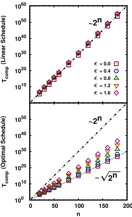
FIG. 1. Even in the presence of discrete local noise, the adiabatic QC is faster than any classical algorithm for searching an unstructured database. The proposed method is applied to calculate the computational time neces-sary to solve the Grover search problem in presence of local disorder. The computational scaling is compared, for increas-ing strength of the local noise, to the best classical result (Tcomp ∝N, whereN = 2n is the number of entries in the
database) and the best quantum result in the ideal case where the noise is absent (Tcomp ∝
√
N). We consider two annealing schedules, the linear one (Top panel) and an optimal sched-ule determined by imposing the adiabatic condition locally (Bottom panel). A quantum speedup is possible only when optimal schedules are adopted. These results are obtained by using the standard driver Hamiltonian, but similar curves have been also obtained for the Grover-style driver Hamilto-nian.
gap g(s) at any point during the evolution. The results are expressed in terms of the computational timeTcomp, namely the temporal cost for the quantum algorithm to reach the success probability of 99% [29, 43].
B. Calculation of the computational time
In general terms, the performance of an adiabatic quantum optimizer is expected to improve if the evo-lution time is increased, since the conditions behind the adiabatic quantum theorem are better satisfied. How-ever, it may be possible that a larger probability of suc-cess is achieved if the adiabatic quantum optimizer is used for a shorter evolution time, but in repeated runs [29, 43]. In Appendix A, we provide a precise analysis of the computational time required to achieve a solution in the general case of an arbitrary adiabatic quantum optimization. To make the definition of computational time (see Appendix A) more concrete, let us apply it to the Grover problem with local disorder and calculate the computational time according to Eq. (A8). Given a tar-get state and a specific realization of the local disorder, the noise term can either increase or decrease the tar-get state energy according to the number q ∈ [0, n] of spins where the disorder provides a positive energy con-tributions. Assuming thati =± are randomly drawn with 50:50 probability, the probability distribution forq
results
pn(q) = 2−n n
q
, (27)
wherenis the number of qubits, while the success prob-ability reads
pS(q, T|q∗) =δ(q−q∗) Θ(T−Tann(q∗)) Θ(q−q), (28) in which the second Θ function takes into account that the target state is the ground state of the noisy Hamil-tonian only forq≤q, withq=b2nc.
Unlike the case of the standard driver Hamiltonian for which the calculation of Tann is not trivial, for the Grover-style driver Hamiltonian we can provide an ac-curate estimate of Tcomp, given that Tann =
√ 2n re-gardless the problem Hamiltonian [49]. Recalling that limn→0pn(q) = 0 (observe that even the mode of the distribution pn(q) scales like maxqpn(q) ≈ 1/
√
n), the computational times becomes
Tcomp() = √
2nmin q∗
n log(1−0.99) log(1−pn(q∗)Θ(q−q∗)))
o
≈log(1−0.99) min 0≤q∗≤q
n
23n/2−n h(q∗/n)o,
(29)
where we used the Stirling approximation log2 nq ≈
n h(q/n) in which
h(x) =−xlog2x−(1−x) log2(1−x) (30) is the Shannon entropy. Finally, the computational scal-ing is
s() = lim n→∞
1
nlog2Tcomp()
=
(1
2 <˜ 3
2−h 1 2
where ˜= 1 is the noise threshold such that the minimum energy of Hdis becomes comparable with the energy of the target state. Interestingly, it exists a noise threshold
cl ≈ 4.54 such that s()≥ 1 for > cl, aka the AQO cannot perform better than classical computers in that regime. Indeed, for large, the probability of the target state to be the true ground state of HAQO with noise becomes smaller. Therefore, minimizingHAQO becomes less efficient than simply trying to find the target state by an exhaustive enumeration. We note that such effect is somewhat artificial since the success probability for very short evolution times tends to 2−n and not to zero as we, conservatively, assumed.
Observe that a more elaborate annealing schedule can partially remove the necessity of repeating runs. In fact, if the annealing schedules(t) is chosen to be the solution of the following equation
ds
dt =minq g
2(s, q), (32)
then it is guaranteed that the quantum dynamics is adia-batic, regardless the hidden parameterq. The evolution time for a single run is expected to increase only lin-early innas compared to the schedule considered above. However, for sufficiently large strength of the noise, fluc-tuations can affect the energy landscape of the problem Hamiltonian with the consequence that the global ground state of the noisy problem Hamiltonian is not anymore the desired target state. In these cases, even for a very slow quantum adiabatic evolution, the final state will not correspond to the target state regardless the evolution time. By quenching the noise and repeating the evo-lution run such problem is naturally solved since more favorable noise realizations are possible.
C. Scaling analysis
In this Section we present our main results on the computational scaling of the noisy Grover problem. Fig. 1 shows the scaling behavior ofTcompby varying the level of noise, using either a linear schedule (Top) or an optimal schedule (Bottom) tailored to the noise model, but independent of the specific target state |σ∗i (see Appendix C and D). In both cases we employ the stan-dard driver Hamiltonian. We observe that, for the linear schedule, neither quantum speedup nor noise effects are observed. The optimal schedule, instead, gives rise to a quadratic quantum speedup in the noiseless case that is, interestingly, only partially canceled when local disorder is taken into account. We also compared the performance of an adiabatic quantum optimizer when the standard driver Hamiltonian is substituted with the Grover-style driver Hamiltonian, in order to see how much the choice of the driver influences the “robustness” of the AQO to local noise (see Fig. 2): In this case, the Grover-style driver preserves all the quadratic quantum speedup if
Lower bound for the quantum calculation Classical regime
0.5
0.6
0.7
0.8
0.9
1.0
0.0
1.0
2.0
3.0
4.0
5.0
6.0
Scaling of the computational time
Standard driver Grover driver
[image:9.612.324.556.51.268.2]Grover driver (analytic estim.)
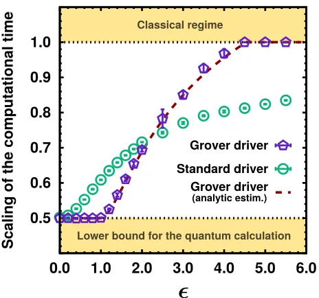
FIG. 2. Polynomial quantum speedups are retained even in the presence of local disorder.The figure shows the behavior of the coefficient characterizing the exponential scaling for the Grover search problem against the strength of the disorder. We adopt an optimal schedule that would guar-antee a quadratic speedup in absence of noise. We find that adiabatic QC still retains a better scaling than any classical algorithm even if the quantum speedup is reduced for increas-ing level of disorder. Interestincreas-ingly, although the Grover-style driver Hamiltonian gives better performances for weak noise, the standard driver Hamiltonian results more “robust” for large noise. The exponential coefficient has been obtained by fittingTcomp for systems up ton≤160 qubits.
the noise is maintained below a certain threshold.˜, but the AQO speedup quickly degrades for moderate disorder until the classical scaling is finally reached. The turning point ˜ ≈ 1 corresponds to the noise threshold for which the lowest energy ofHdis is comparable with the energy of the target state (see Appendix C for more details). Conversely, the standard driver Hamiltonian appears significantly more “robust” at large disorder, so that the performance of the adiabatic QC gently decreases for increasing strength of the noise. These are good news for the possibility of implementing adiabatic QC in realistic systems since one can retain all the quantum speedup (for very weak disorder) or most of it (for moderate disorder) by choosing the appropriate driver Hamiltonian.
In the following, we analyze the effect of different driver Hamiltonians by observing the behavior of the minimum gap at various q/n ratios for the specific system size
x
x
x
x
x
[image:10.612.62.293.48.227.2]x
FIG. 3. Minimum gap calculated for both the standard driver and Grover driver Hamiltonian applied to the Grover search problem with local disorder. In the first case, gmin
spans several orders of magnitude if eitherqorare varied. In the latter case, the minimum gap is, instead, almost constant and scales asgmin= 1/
√
2n. This plot is obtained for systems
ofn= 160 qubits. The symbols are plotted only for thoseq/n
such thatq < q.
for its nature,HD(G)does not see any underlying structure of the problem energy landscape, not even the noise con-tribution, and presents a minimum gap only influenced by the degeneracy of the ground state (in our case, we have a unique ground state as long as q ≤q). On the contrary, the energy landscape plays a role during the adiabatic evolution withHD(S)and this can be easily ob-served for the special case q= 0. In this case, Eq. (C3) assumes the form
HAQO0 =−sn|0ih0| −
n X
i=1 h
s|i|σˆzi + (1−s)ˆσ x i
i
, (33)
and the target state |0ih0| is also the ground state of −Pn
i=1s|i|σˆiz. For small1 one recovers the case of the noiseless Grover problem, while for large 1 the situation is analogous to the Hamming weight problem that presents a gap largely independent of n. The fact that the absolute value of the minimum gap at small
q/n is always larger for the standard driver (even for
<1 when the scaling of the computational time is better with the Grover driver) can be understood observing that the size of the minimum gap is only one of three factors that influence Tcomp; the other two being the shape of the minimum gap (especially its width in the adiabatic coordinate s) and the probability that a certain q/n is realized in practice.
VI. CONCLUSIONS
Estimation of the computational power of the adia-batic quantum optimization requires the knowledge of
the spectral gap of the total Hamiltonian HAQO(s). Its direct quantification is a hard task since it requires the calculation of eigenvalues of matrices which are exponen-tially large in the number of qubits. To circumvent this limitation, several methods have been proposed to di-minish the classical resources necessary to represent the adiabatic quantum optimizer. However, these special-purpose approaches are based on the exploitation of sym-metries of either the driver or the problem Hamiltonian, and are therefore confined to particular classes of prob-lems.
Here, we present and discuss a method that reduces the effective dimensionality of the system even in ab-sence of explicit symmetries, and that goes beyond the idea of studying the properties and structure of the driver and problem terms separately. Formally, this is made possible by the identification of a hidden block diagonal structure in the total Hamiltonian and, consequently, by the existence of a small subspace in which the relevant eigenstates are effectively confined. According to the spe-cific total Hamiltonian HAQO, the present method re-quires only the knowledge of quantities that can be com-puted either analytically or by using efficient numerical approaches.
We apply the proposed method to calculate the en-ergy gap, in a numerically exact way, for large systems exposed to local disorder or other forms of imprecision in the values of the parameter that characterize the problem Hamiltonian: Interestingly, we show that adiabatic quan-tum computation seems to be robust enough to deal with a form of stochastic local noise that is hardly avoidable in any real quantum device. We also find that, although the Grover driver Hamiltonian is potentially faster in the weak noise limit, the standard driver Hamiltonian, which is actually more suitable to be implemented in existing quantum hardware, results less sensitive to discrete noise.
ACKNOWLEDGMENTS
The authors thank Peter J. Love and Sergey Knysh for many useful discussions. This work was supported by the Air Force Office of Scientific Research under Grants FA9550-12-1-0046. A.A.-G. was supported by the Na-tional Science Foundation under award CHE-1152291. A.A.-G. thanks the Corning Foundation for their gener-ous support. The authors also acknowledge the Harvard Research Computing for the use of the Odyssey cluster.
AUTHOR CONTRIBUTIONS
S.M. and A.A.G. designed the research; S.M and G.G.G designed and devised the software for the numerical analysis, performed the research and ana-lyzed the data; S.M, G.G.G and A.A.G. wrote the paper.
APPENDIX
Appendix A: Definition of “computational time” for an adiabatic quantum optimizer
In this appendix Section we provide a precise analysis of the concept of computational time required to achieve a solution of the problem at hand. In particular, we are interested to the case in which a larger probability of suc-cess may be achieved if the adiabatic quantum optimizer is used for a shorter evolution time, but in repeated runs [29, 43]. This strategy trivially includes the possibility of performing a unique, long optimization run.
Let us define pS(T) as the probability of success of the adiabatic quantum optimizer at fixed evolution time
T. Recalling that the probability to (always) fail afterk
attempts is given by (1−pS(T))k, the minimum number
K(T) of attempts to have a probability of 99% to find the correct solution (at least once) results
K(T) = log(1−0.99) log(1−pS(T))
, (A1)
which leads to the definition of the computational time:
Tcomp= min
T n
T·K(T)o= min T
n
T· log(1−0.99) log(1−pS(T))
o
.
(A2) As one can deduce from its definition, it is clear that
Tcomp≤T∗, whereT∗is the minimum evolution time to havepS(T∗) = 0.99.
Consider now the case in which the quantum adiabatic optimizer has a hidden parameter q, which is different from run to run and extracted from a distributionp(q). To give an explicit example, q might take into account how the stochastic local noise relates to the target state for the Grover problem, as described in Section V. In this case, the probability of success of the quantum optimizer has to be averaged over the possible values of the hidden parameter and becomes
¯
pS(T) = X
q
p(q)pS(q, T), (A3)
where pS(q, T) is the probability of success at fixed q. Consequently, the computational time takes the form
Tcomp= min
T n
T· log(1−0.99) log(1−p¯S(T))
o
. (A4)
Assume that, for any given q, it is possible to exactly compute the spectral gapg(s, q) at any time stepsof the adiabatic optimization. Therefore, an optimal schedule tailored for that specific q can be constructed, as de-scribed in [9], which has an optimal evolution time given by
Tann(q)∝ Z 1
0
ds
g2(s, q). (A5)
Since the calculation of the probability of success in Eq. (A3) requires the evolution of the initial quantum state throughout the whole adiabatic calculation, we adopt two main simplifications to avoid this extra over-head. First, we assume that the optimal schedule ob-tained for a specificq∗ is not a good adiabatic schedule for any other q 6= q∗, i.e. that the probability of any otherq6=q∗ isidentically zero
pS(q, T|q∗) =δ(q−q∗)pS(q∗, T|q∗). (A6) Second, we reduce the probability of success for q∗ to
be a step function which is different from zero only if
T > Tann(q∗), namely
pS(q∗, T|q∗) = Θ(T−Tann(q∗)). (A7) Notice that both the above simplifications are quite con-servative since we exclude the possibility that an optimal schedule works (even partially!) for any otherqand that the probability of success is strictly zero even for moder-ate evolution times. Combining Eq. (A6) and Eq. (A7), the computational time in Eq. (A2) assumes the form
Tcomp= min
T n
T· log(1−0.99) log(1−p¯S(T))
o
= min T , q∗
n
T· log(1−0.99) log(1−p(q∗)Θ(T−T
ann(q∗))) o
= min q∗
n
Tann(q∗)·
log(1−0.99) log(1−p(q∗)))
o
. (A8)
It is important to notice that Eq. (A8) depends only on quantities likeTann(q∗) andp(q∗) which are properties of the model and not of the single run. For example, for the Grover problem with noise in Section V, both Tann(q∗) andp(q∗) are completely determined by the noise model.
Appendix B: “Tunneling” model: Barrier around global minimum
Here, we want to study a simple model that can be exactly solved using the exponential reduction method. The peculiarity of this model is that the ground state of the problem is surrounded by a “high-energy barrier” and, therefore, is hard to reach for a classical simulated annealer. However, AQC might find the ground state very quickly due to the tunneling effect as conjectured in Ref. [36, 58]. This example also demonstrates that our method can give rise to an exponential reduction in the dimensionality even for problems where the gap be-haves sub-exponentially, i.e. when the gap closes only polynomially.
Consider the simple problem Hamiltonian correspond-ing to the Hammcorrespond-ing weight problem
HP =− n X
i=1 ˆ
which has a unique ground state, namely the configura-tion with all spins pointing up, and a very simple energy landscape. The main idea is to add a barrier around this unique ground state, that is to say we want to add a potential of the form
V(σ) = (
Vα ifw(σ) = 1
0 otherwise, (B2)
withα={1, . . . , n}the position of the single spin which is pointing down, Vα>0 (butVα<0 can be also used) andw(·) the Hamming weight function. Let us define|αi as the state in which all the spins are up apart from the
α−th spin which points down. Therefore, the problem Hamiltonian becomes
HP =− n X
i=1 ˆ
σiz+ n X
α=1
Vα|αihα|. (B3)
Using the standard driver Hamiltonian HD(S) = −Pn
i=1σˆ
x
i, the AQO Hamiltonian results
HAQO=−(1−s)
n X
i=1 ˆ
σxi −s
n X
i=1 ˆ
σzi +s
n X
α=1
Vα|αihα|
=−ps2+ (1−s)2
n X
i=1
Hi(s) +s n X
α=1
Vα|αihα| (B4)
=−ps2+ (1−s)2
n X
i=1
Hi(s) +s HB,
where HB is the barrier term and all Hi(s) are identi-cal single spin operators which act on thei−th spin and whose explicit expression is given by:
Hi(s) =√ 1−s s2+(1−s)2σˆ
x i +
s
√
s2+(1−s)2σˆ z i
= cos(ϕs)ˆσxi + sin(ϕs)ˆσzi . (B5)
Since eachHi(s) is a rotated Pauli matrix, it has
eigen-values±1 with corresponding eigenstates
φ+s
= √1
2 p
1 + sin(ϕs)|0i+ p
1−sin(ϕs)|1i
= cos(θs)|0i+ sin(θs)|1i
φ−s
= √1 2
p
1−sin(ϕs)|0i − p
1 + sin(ϕs)|1i
= sin(θs)|0i −cos(θs)|1i, (B6)
withθs = ϕ2s. Let us call φ+i (s)
and φ−i (s)
the two eigenstates ofHi(s) for anys. At this point, it is simple to understand that the HamiltonianPn
i=1Hi(s) has ex-actlyn+ 1 energy levels characterized by the number of
φ +
i (s)
andφ−i (s)
states in the product eigenstate. In the{|φ±i} basis, the states in the computational basis can be written as
|0i= cos(θs) φ+s
+ sin(θs) φ−s
(B7a) and
|1i= sin(θs) φ
+
s
−cos(θs) φ−s
. (B7b)
It is important to observe here that all the θs depend only onsand not on the spin indexisince all localHi(s) are identical. Interestingly, the Hamiltonian in Eq. (B4) is the sum of two parts: an Hamiltonian for which we know exactly the eigenenergies/eigenstates for anysand an Hamiltonian which non trivially acts only onnstates. Therefore, this model can be exponentially reduces by using our method.
Before writing the explicit form of the overlap matrix, we introduce a simplified notation in which k(E) rep-resent the number of |φ−
si states in each eigenvalue of energy E of P
iHi(s). With intuitive change of nota-tion:
E(k) = 2k−n, PΩE(k)=Pk,
Zα(E(k)) =Zα(k),
|E(k)αi=|kαi=
Pk|αi
Zα(k)
,
λE(k)=λk= n
k
. (B8)
Zα(k) = p
hα|PΩE|αi =
q n k
qk n|
φ−s 1
|2|
φ−s 0
|2(k−1)|
φ+s 0
|2(n−k)+n−k n |
φ+s 1
|2|
φ−s 0
|2k|
φ+s 0
|2(n−k−1)
= q
n k
|cos(θs)|n−k|sin(θs)|k q
k ntan
−2(θ
s) +n−nktan2(θs) (B9)
kα k0β
=δkk0
1 Zα(k)Zβ(k)
hα|Pk|βi
=δkk0Oαβ(k). (B10)
The last line of Eq. (B10) can be considered as the defini-tion of the overlap matrixOgiven in the basis{|kαi}α,k.
The explicit expressions for the overlap matrix is (includ-ing the normalization):
Oαα(k) = 1,
Oαβ(k) = 1
n−1
−2k(n−k) +k(k−1) tan−2(θ
s) + (n−k)(n−k−1) tan2(θs)
ktan−2(θs) + (n−k),tan2(θs)
(B11)
where, obviously, β 6=α. Observe that the overlap ele-ment does not directly depend onα, β.
Finally, adopting the same notation as in Section IV C
we obtain the explicit form of both terms composing the
reduced HamiltonianHeffin the basis{|Eµi}
notice that
in our simplified notation we have Eµ0
≡
E (E0)
µ E
:
hEµ|HB| Eν0i= n X
α=1
VαhEµ|αi hα| Eν0i=Zα(E)Zα(E0) n X
α=1
VαhEµ|Eαi hEα0 | Eν0i
=Zα(E)Zα(E0) n X
α=1
VαTµα(E)T(E
0)∗
να !
=Zα(E)Zα(E0) h
T(E)T(E0)†i
µν , (B12a)
hEµ|ΣiHi(s)| Eν0i=E δEE0δµν. (B12b)
Where α, β = 1, . . . , n are the indices corresponding to the states in HB = Pnα=1Vα|αihα|, while µ, ν = 1, . . . , κ(E) are the indices labeling the orthonormal basis states of the effective subspace of each ΩE (i.e. neglect-ing the state spannneglect-ingωE).
Appendix C: Grover Problem with local noise (Standard Driver)
In this appendix Section, we will show how to apply our method for the Grover problem in presence of lo-cal noise when the standard driver Hamiltonian is used. In the next Section, we will show briefly the derivation when a Grover-style driver Hamiltonian is used instead.
Consider the following Grover problem Hamiltonian
HP =−n|ωihω|+Hdis, (C1) where Hdis = P
n
i=1iσˆzi plays the role of local disor-der. If the standard driver Hamiltonian is used, the AQO Hamiltonian results
HAQO=−sn|ωihω|+s
n X
i=1
iσˆiz−(1−s) n X
i=1 ˆ
σix. (C2)
is exponentially reduced (compared to 2n), even in pres-ence of local disorder. It is important to stress that our method allows the calculation of the spectral gapwithout any perturbative expansion around the small noise limit. To begin with, let us apply a unitary transformation on Eq. (C3) in order to get rid of the sign of alli, namely
HAQO0 =−sn|ω0ihω0| −s
n X
i=1
|i|σˆzi −(1−s) n X
i=1 ˆ
σix
=−sn|ω0ihω0| −
n X
i=1 h
s|i|σˆiz+ (1−s)ˆσ x i
i
=s HB+γ(s)HA. (C3)
whereγ(s) =p(s||)2+ (1−s)2and
HA=− n X
i=1
s|i|
γ(s)σˆ z i +
(1−s)
γ(s) σˆ x i
, (C4a)
HB =−n|ω0ihω0|. (C4b) Since we want to maintain the number of energy levels of
HA polynomial in the number of spins, we will consider the simple case where the noise is binomial, akai=||δi withδi=±1. Observe that it is possible to have an ex-ponential reduction even if the value of any|i|is chosen from a finite set ofpdistinct (possibly incommensurable) values: In this case, the number of energy levelsM ofHA is upper bounded byM ≤(n+ 1)p.
Therefore, the HamiltonianHB in Eq. (C3) becomes
HA=− n X
i=1 h
sin(ϕs) ˆσiz+ cos(ϕs) ˆσxi i
=−
n X
i=1 ˆ
σi(s), (C5) with sin(ϕs) =
s||
γ(s) and cos(ϕs) = (1−s)
γ(s) . As shown in Appendix B, all the ˆσi(s) are identical and their eigen-states (corresponding to the eigenvalues±1) are
φ+s
=√1
2 p
1 + sin(ϕs)|0i+ p
1−sin(ϕs)|1i
= cos(θs)|0i+ sin(θs)|1i, (C6a)
φ−s
=√1 2
p
1−sin(ϕs)|0i − p
1 + sin(ϕs)|1i
= sin(θs)|0i −cos(θs)|1i. (C6b)
By inverting the above expressions, states in the compu-tational basis can be expressed as
|0i= cos(θs) φ+s
+ sin(θs) φ−s
, (C7a)
|1i= sin(θs) φ+s
−cos(θs) φ−s
. (C7b)
Let us assume thatq=|ω0|. Since the contributionHA to the Hamiltonian HAQO0 as expressed in Eq. (C3) is invariant by spin exchange, we can always assume that all the spins inω0 are ordered, namelyω0 =|0· · ·01· · ·1i (but note that the total HamiltonianHAQO0 still violates the spin exchange symmetry!). Using the same notation as introduced in Appendix B, we write
E(k) = 2k−n, PΩE(k) =Pk,
ZE(k)=Zk,
|E(k)i=|ki=Pk|ω
0i
Zk
,
λE(k)=λk = n
k
, (C8)
wherekis formally the number of|φ−siin a given eigen-state of HB at energy E. λk is the degeneracy of the energy levelE. Given the Hamiltonian in Eq. (C5) and an arbitrary state in the computational base |ω0i, the normalization factorZk can explicitly computed:
Z2
k =hω0|Pk|ω0i=
min{k, q}
X
l=0 q
l
n−q
k−l
sin(θs)2(q−l)+2(k−l)cos(θs)2n−2(q−l)−2(k−l). (C9)
Observe that if sin(θs) = cos(θs) = √12 (namely when the disorder |i| →0), the normalization factor becomes
Zk= 2−n/2 q
n k
for any choiceω0, as expected.
Appendix D: Grover Problem with local noise (Grover-style Driver)
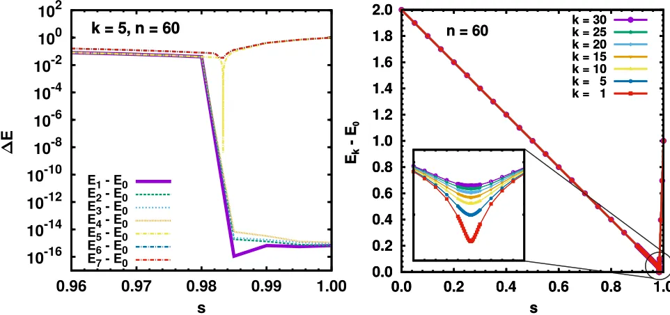
FIG. 4. Application of the proposed reduction method for the multi-solutions Grover problem. (Left panel) Difference in energy between the ground state and thel−th excited state, at fixed number of solutionsk = 5 and number of spinsn= 60. (Right panel) Difference in energy between the ground state and thek−th excited state, by varying the number of solutionsk at fixed number of spinsn= 60.
of noise, when a Grover-style Hamiltonian is used instead of the standard driver Hamiltonian (see Section C). Ob-serve that since the partitioning of theHAQO is different in the two cases, the final reduced Hamiltonian have com-pletely different forms. As in Section C, let us consider the following Grover problem Hamiltonian
HP =−n|ωihω|+Hdis, (D1) where Hdis=Pni=1iσˆzi plays the role of local disorder. Adding the Grover-style driver Hamiltonian, the AQO Hamiltonian results
HAQO=−sn|ωihω|+s
n X
i=1
iˆσiz−(1−s)|ψ0ihψ0|, (D2)
where|ψ0i= √1
2n
P
z|ziis the equal superposition of all the states in the computational basis. After the appli-cation of an unitary transformation to get rid of all the sign ofi, the AQO Hamiltonian becomes
HAQO0 =−sn|ω0ihω0| −s
n X
i=1
|i|σˆzi −(1−s)n|ψ0ihψ0|
=n−s|ω0ihω0| −(1−s)|ψ0ihψ0|−s
n X
i=1 |i|σˆzi
=HB+s HA, (D3)
where
HA=− n X
i=1
|i|ˆσiz, (D4a)
HB=−n
s|ω0ihω0|+ (1−s)|ψ0ihψ0|
. (D4b)
As in Section C, we choose i = ||δi with δi = ±1. Therefore, HA assumes the simple form of a rescaled Hamming weight function, namely:
HA=−|| n X
i=1 ˆ
σiz. (D5)
Once definedE(k) = 2k−nandPk respectively the en-ergy and the projector of the eigenspaces of HA, it is straightforward to follow Section IV C and identify the relevant states in order to construct the reduced Hamil-tonian:
|Eki=
Pk|ψ0i Zk
, (D6a)
Zk= 2−n/2 s
n
k
, (D6b)
|ω0i=α|Eqi+ p
1−α2|Ei, (D6c)
whereq is the Hamming weight of ω0, α= 1/q nqand |Ei is an appropriate eigenstate which is orthogonal to |Eqiand lives in thek−th eigenspace ofHA. Notice that the presence of|ω0iin Eq. (D3) adds only one extra states (formally|Ei) becausePk|ω0i=δkq|ω0i, whereδkqis the Kronecker delta.
Appendix E: Grover problem with multiple solutions
(i.e. target states) are acceptable. As described in Sec-tion IV B, the AQO Hamiltonian for the multi-soluSec-tion Grover problem using the standard driver Hamiltonian can be restricted to at most k ×n orthogonal states, wherekand nare, respectively, the number of solutions and the number of spins composing the database register.
Let{|w1i, . . . , |wki}being the states representing the solutions of the Grover problem. Their projections onto the eigenspaces of the standard driver Hamiltonian can be written as
|Eαi=
PΩE|wαi Zα(E)
= s
1/
n
u(E)
X
x|w(x)=k
(−1)x·w|wi,
(E1) where u(E) = (E+n)/2 represents the number of spin up at a given energy E of the driver Hamiltonian, x is an arbitrary bit configuration, andw(x) is the Hamming weight. After some combinatorial analysis, the overlap
matrixhEα|Eβiresults to be:
hEα|Eβi= 1/ n
u(E)
min{dαβ, u(E)}
X
l=0
(−1)l d
αβ
l
n−d αβ
u(E)−l
,
(E2) wheredαβ is the Hamming distance betweenωαandωβ. As expected, ifd= 0 the overlap is identically 1, as well as ifu(E) = 0.
In Fig. 4, left panel, we show the difference in energy between the ground state and the l−th excited state, at fixed number of solutions k = 5 and number of spins n = 60, while in the right panel we show the difference in energy between the ground state and the
k−th excited state, by varying the number of solutions
k at fixed number of spins n = 60. As expected, the energy spectrum is k−degenerate at s = 1, meaning that all thek solutions belong to the reduced subspace obtained through our method to exponentially reduced the effective dimensionality.
[1] Edward Farhi, J. Goldstone, S. Gutmann, J. Lapan, A. Lundgren, and D. Preda. A quantum adiabatic evolu-tion algorithm applied to random instances of an NP-complete problem. Science, 292(5516):472–475, April 2001.
[2] P. Ray, B. K. Chakrabarti, and Arunava Chakrabarti. Sherrington-Kirkpatrick model in a transverse field: Ab-sence of replilca symmetry breaking due to quantum fluc-tuations. Physical Review B, 39(16):11828, 1989. [3] Tadashi Kadowaki and Hidetoshi Nishimori. Quantum
annealing in the transverse Ising model. Physical Review E, 58(5):5355, 1998.
[4] A. B. Finnila, M. A. Gomez, C. Sebenik, C. Stenson, and J. D. Doll. Quantum annealing: A new method for min-imizing multidimensional functions. Chemical Physics Letters, 219(March):343–348, 1994.
[5] Yong-Han Lee and B. J. Berne. Global optimization: Quantum thermal annealing with path integral Monte Carlo. The Journal of Physical Chemistry A, 104(1):86– 95, 2000.
[6] Ryan Babbush, Alejandro Perdomo-Ortiz, B. O’Gorman, William G. Macready, and Al´an Aspuru-Guzik. Con-struction of energy functions for lattice heteropolymer models: Efficient encodings for constraint satisfaction programming and quantum annealing. Advances in Chemical Physics, 155:201, 2012.
[7] Rolando D Somma, Daniel Nagaj, and M´aria Kieferov´a. Quantum speedup by quantum annealing. Physical re-view letters, 109(5):050501, 2012.
[8] Alejandro Perdomo-Ortiz, Neil Dickson, Marshall Drew-Brook, Geordie Rose, and Al´an Aspuru-Guzik. Find-ing low-energy conformations of lattice protein models by quantum annealing. Scientific reports, 2, 2012. [9] J´er´emie Roland and Nicolas J. Cerf. Quantum search
by local adiabatic evolution. Physical Review A,
65(4):042308, March 2002.
[10] Edward Farhi, Jeffrey Goldstone, and Sam Gutmann. Quantum adiabatic evolution algorithms with different paths. arXiv: quant-ph/0208135, pages 1–10, 2002. [11] Saurya Das, Randy Kobes, and Gabor Kunstatter.
Adi-abatic quantum computation and Deutschs algorithm.
Physical Review A, 65(6):062310, June 2002.
[12] Zhaohui Wei and Mingsheng Ying. A modified quan-tum adiabatic evolution for the Deutsch-Jozsa problem.
Physics Letters A, 354(4):271–273, June 2006.
[13] Boris Altshuler, Hari Krovi, and J´er´emie Roland. Ander-son localization makes adiabatic quantum optimization fail. Proceedings of the National Academy of Sciences, 107(28):12446–12450, 2010.
[14] Vicky Choi. Different adiabatic quantum optimization algorithms for the NP-complete exact cover problem.
Proceedings of the National Academy of Sciences USA, 108(7):E19–20, March 2011.
[15] Wim van Dam, Michele Mosca, and Umesh Vazirani. How powerful is adiabatic quantum computation? Pro-ceedings of the 42nd IEEE Symposium on Foundations of Computer Science, pages 279 – 287, 2001.
[16] Dorit Aharonov, Wim van Dam, Julia Kempe, Zeph Lan-dau, Seth Lloyd, and O. Regev. Adiabatic quantum com-putation is equivalent to standard quantum comcom-putation.
SIAM Review, 50(4):755–787, 2008.
[17] David Deutsch and Richard Jozsa. Rapid Solution of Problems by Quantum Computation.Proc. R. Soc. Lond. A, 439(1907):553–5585, 1992.
[18] Lov K. Grover. A fast quantum mechanical algorithm for database search. Proceedings of the Twenty-Eighth Annual ACM Symposium on Theory of Computing STOC 96, 1996.
com-puter. SIAM Review, 41(2):303–332, 1999.
[20] Daniel S. Abrams and Seth Lloyd. Quantum algo-rithm providing exponential speed increase for finding eigenvalues and eigenvectors. Physical Review Letters, 83(24):5162–5165, December 1999.
[21] Tad Hogg. Adiabatic quantum computing for random satisfiability problems. Physical Review A, 67(2):022314, February 2003.
[22] Alejandro Perdomo-Ortiz, Salvador E. Venegas-Andraca, and Al´an Aspuru-Guzik. A study of heuristic guesses for adiabatic quantum computation. Quantum Information Processing, 10(1):33–52, March 2010.
[23] Itay Hen and AP Young. Solving the graph-isomorphism problem with a quantum annealer. Physical Review A, 86(4):042310, 2012.
[24] Elizabeth Crosson, Edward Farhi, Cedric Yen-yu Lin, Han-hsuan Lin, and Peter Shor. Different strategies for optimization using the quantum adiabatic algorithm.
arXiv: 1401.7320, (4):1–17, 2014.
[25] Al´an Aspuru-Guzik, Anthony D Dutoi, Peter J Love, and Martin Head-Gordon. Simulated quantum computa-tion of molecular energies.Science, 309(5741):1704–1707, 2005.
[26] M-H Yung, J Casanova, A Mezzacapo, J McClean, L Lamata, A Aspuru-Guzik, and E Solano. From tran-sistor to trapped-ion computers for quantum chemistry.
Scientific reports, 4, 2014.
[27] Jarrod R McClean, John A Parkhill, and Al´an Aspuru-Guzik. Feynman’s clock, a new variational principle, and parallel-in-time quantum dynamics. Proceedings of the National Academy of Sciences, 110(41):E3901–E3909, 2013.
[28] Alberto Peruzzo, Jarrod McClean, Peter Shadbolt, Man-Hong Yung, Xiao-Qi Zhou, Peter J Love, Al´an Aspuru-Guzik, and Jeremy L O’Brien. A variational eigenvalue solver on a quantum processor. Nature Communications, 5(4213), 2014.
[29] Troels F. Rønnow, Zhihui Wang, Joshua Job, Sergio Boixo, Sergei V. Isakov, David Wecker, John M. Marti-nis, Daniel A. Lidar, and Matthias Troyer. Defining and detecting quantum speedup.Science, 345(6195):420–424, 2014.
[30] Giuseppe E Santoro, Roman Martoˇn´ak, Erio Tosatti, and Roberto Car. Theory of quantum annealing of an Ising spin glass. Science, 295(5564):2427–2430, 2002.
[31] DA Battaglia and L Stella. Optimization through quan-tum annealing: theory and some applications. Contem-porary Physics, 47(4):195–208, 2006.
[32] A. Young, S. Knysh, and V. Smelyanskiy. Size de-pendence of the minimum excitation gap in the quan-tum adiabatic algorithm. Physical Review Letters, 101(17):170503, October 2008.
[33] Itay Hen. Excitation gap from optimized correlation functions in quantum Monte Carlo simulations. Physi-cal Review E, 85(3):036705, 2012.
[34] Marko Znidaric and Martin Horvat. Exponential com-plexity of an adiabatic algorithm for an NP-complete problem. Physical Review A, 73(2):022329, February 2006.
[35] Itay Hen. Continuous-time quantum algorithms for un-structured problems.Journal of Physics A: Mathematical and Theoretical, 47(4):045305, January 2014.
[36] Edward Farhi, Jeffrey Goldstone, and Sam Gutmann. Quantum adiabatic evolution algorithms versus
simu-lated annealing. arXiv: quant-ph/0201031, 2002. [37] MHS Amin, Peter J Love, and CJS Truncik. Thermally
assisted adiabatic quantum computation.Physical review letters, 100(6):060503, 2008.
[38] Mohammad H. S. Amin, Dmitri V. Averin, and James a. Nesteroff. Decoherence in adiabatic quantum computa-tion. Physical Review A, 79:022107, 2009.
[39] Neil G. Dickson, M. W. Johnson, M. H. S. Amin, R. Har-ris, F. Altomare, A. J. Berkley, P. Bunyk, J. Cai, E. M. Chapple, P. Chavez, F. Cioata, T. Cirip, P. DeBuen, M. Drew-Brook, C. Enderud, S. Gildert, F. Hamze, J. P. Hilton, E. Hoskinson, Kamran Karimi, E. Ladizinsky, N. Ladizinsky, T. Lanting, T. Mahon, R. Neufeld, T. Oh, I. Perminov, C. Petroff, A. Przybysz, C. Rich, P. Spear, A. Tcaciuc, M. C. Thom, E. Tolkacheva, S. Uchaikin, J. Wang, A. B. Wilson, Z. Merali, and G. Rose. Ther-mally assisted quantum annealing of a 16-qubit problem.
Nature Communications, 4(May):1903, May 2013. [40] Kristen L. Pudenz, Tameem Albash, and Daniel A.
Li-dar. Error-corrected quantum annealing with hundreds of qubits. Nature Communications, 5:3243, February 2014. [41] Albert Messiah. Quantum Mechanics. Wiley, 1958. [42] Sabine Jansen, Mary-Beth Ruskai, and Ruedi Seiler.
Bounds for the adiabatic approximation with applica-tions to quantum computation.Journal of Mathematical Physics, 48(10):102111, 2007.
[43] Sergio Boixo, Troels F. Rønnow, Sergei V. Isakov, Zhihui Wang, David Wecker, Daniel A. Lidar, John M. Martinis, and Matthias Troyer. Evidence for quantum annealing with more than one hundred qubits. Nature Physics, 10(February):218, 2014.
[44] J. Lee. New Monte Carlo algorithm: Entropic sampling.
Physical Review Letters, 71(2):211–214, 1993.
[45] Fugao Wang and D. Landau. Efficient, multiple-range random walk algorithm to calculate the density of states.
Physical Review Letters, 86(10):2050–2053, March 2001. [46] Ronald Dickman and A. G. Cunha-Netto. Complete
high-precision entropic sampling. Physical Review E, 84(2):026701, August 2011.
[47] Lov K. Grover. Quantum mechanics helps in search-ing for a needle in a haystack. Physical Review Letters, 79(2):325–328, 1997.
[48] Edward Farhi and Sam Gutmann. Analog analogue of a digital quantum computation. Physical Review A, 57(4):2403–2406, April 1998.
[49] Edward Farhi, Jeffrey Goldstone, Sam Gutmann, and Daniel Nagaj. How to make the quantum adiabatic algo-rithm fail. International Journal of Quantum Informa-tion, 6(03):503–516, 2008.
[50] Lawrence M Ioannou and Michele Mosca. Limitations of some simple adiabatic quantum algorithms.International Journal of Quantum Information, 6(03):419–426, 2008. [51] Zhenwei Cao and Alexander Elgart. On the efficiency
of hamiltonian-based quantum computation for low-rank matrices.Journal of Mathematical Physics, 53(3):032201, 2012.
[52] P. W. Anderson. Local moments and localized states.
Reviews of Modern Physics, 50(2):191–201, 1978. [53] Neil Shenvi, Kenneth R. Brown, and K. Birgitta Whaley.
Effects of noisy oracle on search algorithm complexity.
Physical Review A, 68:052313, 2003.
[55] Markus Tiersch and Ralf Sch¨utzhold. Non-Markovian decoherence in the adiabatic quantum search algorithm.
Physical Review A, 75:062313, 2006.
[56] Davide Venturelli, Salvatore Mandr`a, Sergey Knysh, Bryan OGorman, Rupak Biswas, and Vadim Smelyan-skiy. Quantum optimization of fully connected spin glasses. Physical Review X, 5(3):031040, 2015.
[57] Andrew D King and Catherine C McGeoch. Algorithm
engineering for a quantum annealing platform. arXiv preprint arXiv:1410.2628, 2014.