RESEARCH ARTICLE
10.1002/2014JC010324
Modeling the impact of glacial runoff on fjord circulation and
submarine melt rate using a new subgrid-scale
parameterization for glacial plumes
Tom Cowton1, Donald Slater2, Andrew Sole1, Dan Goldberg2, and Peter Nienow2
1Department of Geography, University of Sheffield, Sheffield, UK,2School of Geosciences, University of Edinburgh, Edinburgh, UK
Abstract
The injection at depth of ice sheet runoff into fjords may be an important control on the frontal melt rate of tidewater glaciers. Here we develop a new parameterization for ice marginal plumes within the Massachusetts Institute of Technology General Circulation Model (MITgcm), allowing three-dimensional sim-ulation of large (500 km2) glacial fjords on annual (or longer) time scales. We find that for an idealized fjord (without shelf-driven circulation), subglacial runoff produces a thin, strong, and warm down-fjord current in the upper part of the water column, balanced by a thick and slow up-fjord current at greater depth. Although submarine melt rates increase with runoff due to higher melt rates where the plume is in contact with the ice front, we find that annual submarine melt rate across the ice front is relatively insensitive to var-iability in annual runoff. Better knowledge of the spatial distribution of runoff, controls on melt rate in those areas not directly in contact with plumes, and feedback mechanisms linking submarine melting and iceberg calving are necessary to more fully understand the sensitivity of glacier mass balance to runoff-driven fjord circulation.1. Introduction
The melting of Greenland’s marine terminating glaciers by warm oceanic waters may be a significant cause of dynamic mass loss from the Greenland ice sheet [Holland et al., 2008;Straneo and Heimbach, 2013]. Rela-tively little is however known about this process, particularly the interaction between the glacier (and sub-glacial runoff), fjord circulation, and terminus melt rates [Straneo et al., 2013]. For example, although very high (>5 m d21) melt rates have been predicted in areas directly adjacent to upwelling subglacial runoff [Jenkins, 2011;Xu et al., 2012], the importance of this process when considered across the entirety of the gla-cier front remains unclear. The significance of glacially forced estuarine circulation within the fjords as a means of replenishing the supply of warm water available for melting at the fjord head is also debated [e.g.,
Motyka et al., 2013;Straneo et al., 2010].
Obtaining field measurements from Greenland’s ice-choked fjords has proven extremely difficult, particu-larly in the critical area close to glacier fronts [Straneo et al., 2013]. As such, data sets of water properties [e.g.,Chauche et al., 2014;Mortensen et al., 2011;Rignot et al., 2010;Straneo et al., 2011, 2010] are rare and often limited with regard to timeframe and proximity to the glacier, making interpretation challenging. The convection of glacial plumes was modeled byJenkins[2011], providing a theoretical relationship between meltwater discharge and submarine melt rate, but this approach cannot provide information on the impact of such plumes on the wider fjord circulation. In recent years, numerical ocean models have also been used to examine the impact of glacial runoff on fjord circulation [Salcedo-Castro et al., 2011;Sciascia et al., 2013;
Xu et al., 2013, 2012]. Such studies have however been limited by the computational expense of both resolv-ing the fine-scale, highly nonhydrostatic dynamics of the turbulent glacial outflow plume and incorporatresolv-ing the wider circulation of fjords that may be hundreds of square kilometers in area. This constraint has resulted in simulations being limited to two-dimensional fjords [Sciascia et al., 2013;Xu et al., 2012] or small (<0.1 km2) three-dimensional domains [Xu et al., 2013], and short (hours to days) simulation times. Here we aim to overcome these constraints by parameterizing the glacial plume. Parameterization of verti-cal motion is a technique commonly employed in ocean modeling, allowing incorporation of processes occurring at a scale finer than the grid resolution [e.g.,Campin and Goosse, 1999;Paluszkiewicz and Romea, Key Points:
We present a method for parameterizing subglacial runoff in ocean models
This is used to examine fjord circulation and glacier melt on annual time scales
We find interannual runoff variability to have only limited impact on melt rate
Supporting Information: Cowton Supporting Information
Correspondence to: T. Cowton,
t.cowton@sheffield.ac.uk
Citation:
Cowton, T., D. Slater, A. Sole, D. Goldberg, and P. Nienow (2015), Modeling the impact of glacial runoff on fjord circulation and submarine melt rate using a new subgrid-scale parameterization for glacial plumes,J. Geophys. Res. Oceans,120, 796–812, doi:10.1002/2014JC010324.
Received 18 JUL 2014 Accepted 7 JAN 2015
Accepted article online 22 JAN 2015 Published online 12 FEB 2015
This is an open access article under the terms of the Creative Commons Attribution-NonCommercial-NoDerivs License, which permits use and distribution in any medium, provided the original work is properly cited, the use is non-commercial and no modifications or adaptations are made.
Journal of Geophysical Research: Oceans
The copyright line for this article was changed on 30 AUG 2016 after original online publication.
1997;Price and Yang, 1998]. We start by developing a plume model based on an input of subglacial runoff from a point source (i.e., a major subglacial channel), as is expected based on the observation of discrete plumes adjacent to tidewater glacier fronts [e.g.,Chauche et al., 2014;Sole et al., 2011]. This is then used to calculate the vertical movement of water, heat, and salt at each time step at a specified location within an ocean model. Doing so eliminates the need to resolve the glacial plume, thus permitting much coarser model resolution. This has the advantage of greatly reducing the simulation time while still allowing the plume to evolve as runoff varies or conditions in the fjord change.
This model is used to examine ice-ocean interaction on annual time scales in an idealized fjord, similar in scale to a large Greenlandic fjord such as Sermilik or Kangerdlugssuaq. Greenland’s glacial fjords are com-plex environments, driven by a range of highly variable terrestrial, atmospheric, and oceanic forcings [ Stra-neo and Heimbach, 2013]. We do not attempt to realistically recreate or assess the relative importance of the multiple components of fjord circulation. Instead we single out the glacial forcing, in particular assessing the impact of glacial melting and runoff on fjord circulation and the sensitivity of submarine melt rate to glacial runoff. In doing so, we seek to aid the interpretation of existing oceanographic data and assess the significance of glacially forced fjord circulation for the future stability of Greenland’s tidewater glaciers. Fur-thermore, this idealized study provides an initial framework in which to develop and test the new plume parameterization, which we envisage applying to complex, realistic fjord systems in future work.
2. Methods
2.1. Model
2.1.1. Ocean Model
The Massachusetts Institute of Technology General Circulation Model (MITgcm, http://mitgcm.org) [Adcroft et al., 2004;Marshall et al., 1997a, 1997b] is a versatile general circulation model that solves the incompressi-ble Navier-Stokes equations using finite-volume methods on an orthogonal curvilinear grid. The model has a nonhydrostatic capability that makes it suitable for the study of areas of complex bathymetry and buoyant upwellings and includes options to incorporate horizontal ice shelves [Losch, 2008] and vertical ice faces [Xu et al., 2012]. To date, it has been used in several studies of glacial ice-ocean interaction both beneath Ant-arctic ice shelves [Heimbach and Losch, 2012;Losch, 2008] and in Greenland’s fjords [Sciascia et al., 2014, 2013;Xu et al., 2013, 2012]. We use the model in nonhydrostatic mode, but the plume parameterization (described in the following sections) is equally suitable for incorporating glacial plumes in relatively coarse hydrostatic simulations.
2.1.2. Plume Model
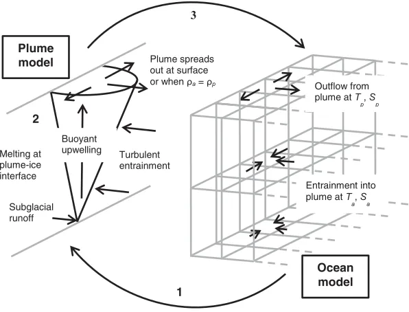
Theoretical models of turbulent plumes have been developed and utilized for over 50 years [e.g.,Morton et al., 1956] and have proven highly effective at representing a wide range of oceanic and atmospheric phenomena [Kaye, 2008]. The plume model that forms the basis of the parameterization is motivated by that ofJenkins[2011], which coupled a buoyant plume model to equations describing heat exchange at the ice-ocean interface.Jenkins’s [2011] model does not include plume expansion or entrainment in an across-fjord direction, and so is only appropriate in scenarios in which the input of runoff is uniform across the width of the glacier. At tidewater glaciers in Greenland, localized turbid plumes have been observed at the fjord surface in summer [e.g.,Chauche et al., 2014;Sole et al., 2011;Tedstone and Arnold, 2012], suggesting the presence of large subglacial channels providing a localized input of runoff to the fjord at the glacier grounding line. As such, an alternative plume geometry, permitting a discrete source of freshwater input, is required (M. O’Leary, Frontal processes on tidewater glaciers, University of Cam-bridge, unpublished thesis, 2011). In these cases, a half-conical plume geometry, with flat side against the glacier, is more appropriate (Figure 1). We therefore construct a model for an ice marginal plume of this geometry utilizing well-established plume theory [Kaye, 2008]. This model is described here, with symbols and parameter values defined in Table 1.
plume velocity with ratea. We employ the standard Boussinesq approximation, which introduces a refer-ence densityq0into the equations. With plume radiusband vertical velocityu, the defining equations (1–4)
state conservation of mass, momentum, heat, and salt:
d dz b
2u
52abu14
pbm_ (1)
d dz b
2u2
5gb2qa2qp
q0 2
4Cd
p bu
2 (2)
d dz b
2uT p
52abuTa1 4
pmbT_ b2
4CTCd1=2
p bu Tp2Tb
(3)
d dz b
2uS p
52abuSa1 4
pmbS_ b2
4CSC1 =2 d
p bu Sp2Sb
(4)
As inJenkins[2011], the last term in (1) and the last two terms in (3) and (4) describe the melting of the ice, and the last term in (2) is a reduction in momentum due to friction, with additional multipliers to take into account the plume geometry.Ta,Sa, andqaare the ambient fjord conditions. The submarine melt ratem_ is related to the
plume variablesTp,Sp, anduand the ice-ocean boundary layer temperatureTband salinitySbusing a three-equation formulation which has frequently been used in this setting [e.g.,Holland and Jenkins, 1999]:
_
m cð iðTb2TiÞ1LÞ5CTC1 =2
d ucw Tp2Tb
(5)
_
mSb5CsC1 =2 d u Sp2Sb
(6)
Tb5k1Sb1k21k3z (7) An analytical solution to the plume equations can be obtained using a number of simplifications (support-ing information). For example, neglect(support-ing the melt and friction terms in (1)–(4) (which is a good approxima-tion for a high initial discharge) and assuming a linear equaapproxima-tion of state and uniform ambient condiapproxima-tions, equations (1–4) have the solution described inStraneo and Cenedese[2015] for a point source plume. This analytical solution can provide physical intuition, but for the more general cases of finite source size,
Subglacial runoff
Plume model
Ocean model
Outflow from plume at Tp, Sp
Entrainment into plume at T
a, Sa
Buoyant
upwelling Turbulent entrainment
Plume spreads out at surface or when ρa=ρp
Melting at plume-ice interface
1 2
[image:3.630.236.534.112.339.2]3
Figure 1.Schematic of the coupled plume-ocean model used in this paper.Ta,Sa,qa5ambient (fjord) temperature, salinity, and density,
Tp,Sp,qp5plume temperature, salinity, and density. (1) At each time step, ambient temperature and salinity profiles are sent from the
stratified ambient conditions, a nonlinear equation of state, and inclusion of the melt and friction terms, the equations must be solved numerically. In this study, we therefore solve the equations numerically using the DLSODE differential equation solver [Hindmarsh, 1983].
In common with the model ofJenkins[2011], the plume emerges vertically into the domain. This is unlikely to occur in reality, and thus it is not clear how to choose the initial plume radiusbiand velocityuifor a given dischargeQ, related in our model byQ5pb2
iui=2. We find however that the model is insensitive to this choice, in that solutions converge quickly on one another for various combinations of (biui) so long asQ remains fixed. Accordingly, we maintain a constantuiof 1 m s21and varybito provide the required discharge.
2.1.3. Integration of the Plume and Ocean Models
To allow the simulation of plumes at subgrid scale, we embed the plume model as a new module within the MITgcm (Figure 1). In grid locations where subglacial runoff is specified, ambient conditions (Ta,Sa,qa) are passed at each time step from the MITgcm to the plume model. These are used, in conjunction with the specified runoff (bi,ui,Ti,Si), to calculate plume radius, velocity, temperature, and salinity as described above. The vertical extent of the plume is also calculated, with the plume terminating upon reaching neu-tral buoyancy or the fjord surface. Water, heat, and salt are then removed from MITgcm cells at the rate pre-dicted by the plume model in those vertical layers where the plume is entraining, and put into the cell at the depth at which the plume is predicted to terminate. Further detail on the model implementation is pro-vided in the supporting information.
[image:4.630.186.584.108.396.2]The primary advantage of this approach over models which seek to resolve the plume is that it permits a relatively coarse spatial and temporal resolution to be used throughout the domain, greatly increasing com-putational efficiency.Xu et al. [2013], for example, required grid cells of 1 m3at the ice front to resolve the plume, necessitating limiting their domain to a section of fjord 500 m long, 500 m deep, and 150 m wide. Such high spatial resolution also requires a very small time step, particularly since vertical plume velocities may exceed 2 m s21[Xu et al., 2013], which again increases the computational demands. Because the plume parameterization presented here undertakes vertical transport outside of the MITgcm framework, the time constraint imposed by high vertical velocities within the model domain is avoided. An additional benefit of
Table 1.Model Parameters
Symbol Name Value Units
ci Heat capacity of ice 2000 J kg
21C21 cw Heat capacity of water 3974 J kg21C21
a Entrainment parameter 0.1
g Gravitational acceleration 9.81 m s21 Ti Ice temperature 210 C
L Latent heat of melting 3.353105
J kg21
UT Thermal turbulent transfer coefficient 2.20310
22
US Salt turbulent transfer coefficient 6.2031024
Cd Ice-plume drag coefficient 2.50310
23
k1 Freezing point slope 25.7331022 C psu21
k2 Freezing point offset 8.32310
22 C
k3 Freezing point depth 7.6131024 C m21
q0 Reference density 1020 kg m
23
qa Ambient density kg m23
qp Plume density kg m
23 Tp Plume temperature C
Sp Plume salinity psu
Tb Boundary temperature C
Sb Boundary salinity psu
u Plume velocity m s21
b Plume radius m
_
m Melt rate m d21
z Depth m
ubg Background velocity 0.01, 0.06, 0.10 m s21
f Coriolis parameter 1.3731024
rad s21 kz Vertical Laplacian diffusivity 1025 m2s21
kh Lateral Laplacian diffusivity 30 m
2 s21 Az Vertical eddy viscosity 1025 m2s21
Ah Lateral eddy viscosity 30 m
this method is that it may improve the prediction of plume dynamics relative to intermediate resolution models (10–20 m horizontal resolution) which seek to resolve the plume, as such models remain highly dependent on viscosity and diffusivity parameterization terms within the ocean model that are difficult to constrain [Sciascia et al., 2013;Xu et al., 2012].
Along the remainder of the ice front, there is melting but no-runoff input. The melt rate in these cells is cal-culated using the same formulation as in the plume model (equations (5–7)) using the temperature, salinity, and velocity as determined by the ocean model. The impact of this melting is taken into account by gener-ating a virtual salinity and heat flux out of the domain, thus cooling and freshening the cells, based on the approach used to incorporate the melting of glacial ice in previous studies using MITgcm [e.g.,Losch, 2008;
Xu et al., 2012]. In reality, this melting would likely establish convective cells against the ice front on spatial scales too small to feasibly resolve in a fjord model [Wells and Worster, 2008]. Although these convective cells are expected to be much weaker than those forced by subglacial runoff (with a vertical extent on the order of 10 m in a stratified ocean environment [Huppert and Josberger, 1980;Jacobs et al., 1981]), it is important that these currents are taken into consideration. This is because they control the melt rate on parts of the calving front not in contact with a runoff-driven plume, which may be the majority of the ice front. As such, in some experiments we specify a minimum velocity in equations (5–7) (similar toXu et al. [2013]). Experiments were undertaken using a minimum velocity of 0.01, 0.06, and 0.10 m s21, based on a range of modeling and field experiments, to assess the influence of this value on the processes simulated in this study (supporting information).
2.2. Initial Fjord Conditions
We utilize temperature and salinity profiles taken in front of Store Glacier, west Greenland, during August 2010 [Chauche et al., 2014] as initial and ocean-boundary conditions for all experiments presented in this paper (Figure 2a). These records, chosen because they provide a detailed survey of temperature and salinity within a few kilometers of the calving front of a major Greenlandic outlet glacier, were averaged to provide representative near-glacier conditions. Although in reality conditions down-fjord may vary from those recorded near to the calving front, we specify horizontally uniform initial conditions. This means that no model spin-up period is required, with initial velocities throughout the domain zero and any subsequent cir-culation resulting from the evolution of water properties over the course of the simulation.
3. Experiments
3.1. Plume Model
As a first step, we examine the plume model independently of the ocean model. Plumes are calculated based on subglacial discharges of 1, 10, and 100 m3s21, using an initial plume temperature of 0C and
0 1 2 3
500 400 300 200 100 0
Temperature (°C)
Depth (m)
a. 32 33 34 35
Salinity (psu)
S T
0 100 200 300 0
100 200 300 400 500 600
Discharge (m
3 s
−1
)
Day of experiment b. 0.5x
1x 1.5x 2x
01Mar 01Jul 01Nov Date
0 100 200 300 0
50 100 150 200 250 300
Discharge (m
3 s
−1
)
Day of experiment c. 01Mar 01Jul 01Nov
[image:5.630.75.559.102.263.2]Date
Figure 2.Initial conditions and forcings used in the model experiments. (a) Temperature and salinity profiles used as initial conditions, derived by averaging Store Fjord profiles taken
salinity of 0 psu and ambient fjord conditions as described in section 2.2. We compare the results to that ofJenkins’s [2011] model, run using the same initial plume conditions, to assess the difference in the model solution generated by the different plume geometries. The horizontal extent of the plume is described in terms of the plume radius in the half-conical model and the thickness of the plume perpen-dicular to the ice front inJenkins’s [2011] model (because of the differing geometry); however, these two variables are directly comparable in terms of the expansion of the plume as it rises through the water column.
The results of the half-conical plume model, along with those from the model byJenkins[2011], are shown in Figure 3. The two models produce similar plume behavior: the plumes expand as they rise, entraining salty water until they become denser than the ambient waters (due to the salinity stratification), which occurs at greater depth for a smaller initial discharge. Because the water column is warmest at depth, both models predict the plumes to be warmer than the ambient conditions above350 m depth. The principal difference between the two models is that our model entrains more rapidly. This is because the half-conical form gives the plume a greater surface area across which to entrain relative to the sheet form ofJenkins’s [2011] model. Because the plume entrains more rapidly, it rises more slowly and reaches neutral buoyancy at a greater depth relative to the sheet model. For example, at a discharge of 10 m3s21,Jenkins’s [2011] model produces a plume that reaches almost to the surface of the fjord, while our modeled plume reaches neutral buoyancy at a depth of70 m. The geometry ofJenkins’s [2011] model requires that the input of runoff is constant across the full width of the grounding line, a scenario that is unlikely to occur in reality at tidewater glaciers given the presence of subglacial drainage channels and uneven bed topography. The 0 20 40 60
500 400 300 200 100 0
Plume radius (m)
Water depth (m)
a. a. a. a. a. a. a. a. a.
0 1 2 3
500 400 300 200 100 0
Vertical velocity (m s−1)
Water depth (m)
b. b. b. b. b. b. b. b. b.
0 1 2 3
500 400 300 200 100 500
Temperature (°C)
Water depth (m)
c. c. c. c. c. c. c. c. c.
0 10 20 30 40 500 400 300 200 100 0 Salinity (psu)
Water depth (m)
d. d. d. d. d. d. d. d. d.
1000 1010 1020 1030 500 400 300 200 100 0
Density (kg m−3)
Water depth (m)
e. e. e. e. e. e. e. e. e.
0 5 10
500 400 300 200 100 0
Melt rate (m d−1)
Water depth (m)
f. f. f. f. f. f. f. f. f.
[image:6.630.74.558.101.443.2]Ambient 10 m3s−1 100 m3s−1 1 m3s−1 10 m3s−1 100 m3s−1
Figure 3.Results generated using the plume model with a freshwater input of 1, 10, and 100 m3
s21
(blue). Also shown for comparison are the plumes generated by the model ofJenkins [2011] using freshwater inputs of 10 and 100 m3
s21
main implication of this therefore is that plumes are likely to reach neutral buoyancy somewhat lower in the water column than predicted byJenkins[2011].
3.2. Coupled Plume-Ocean Model
The next step is to examine the representation of one of these plumes (subglacial discharge5100 m3s21) in the coupled plume-ocean model. The focus of this experiment is across-fjord variation in conditions at the fjord-glacier boundary. To do this, we use a rectangular domain 6.7 km long, 1.8 km wide, and 500 m deep. Grid resolution is 200 m in the cross-fjord direction (chosen such that the width of a cell is compara-ble to the predicted maximum width of the plume) and 10 m in the vertical. In the along-fjord direction, model resolution is 200 m for the 2 km of the domain closest to the glacier, decreasing linearly to 1500 m at the fjord mouth. The sides of the domain are closed, while a glacier extends the full width of the domain at the fjord head, with the plume in the center. A relaxation zone is used to restore properties to the initial conditions at the ocean boundary. The model is run for a simulation time of 1 h, during which time currents generated at the glacier do not reach the ocean boundary.
Initial conditions throughout the domain are set based on the temperature and salinity profiles from Store Glacier (Figure 2a). Diffusivity and viscosity parameters are chosen to be as low as possible without generat-ing numerical noise [Kantha and Clayson, 2000] and are constant between experiments (Table 1; see sup-porting information for assessment of the sensitivity to these and other parameters). In order to assess the impact of cross-fjord circulatory patterns on melt rate, we do not specify a minimum background velocity in this experiment (section 2.1.3).
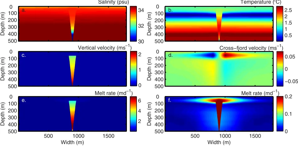
The interaction between the plume and fjord is best seen by looking at the modification of water properties across the ice front (Figure 4). As in the plume model output (Figure 3), the plume forms a zone of relatively fresh, warm water rising up the center of the ice front (Figures 4a and 4b). As it rises, the plume entrains water from the fjord, generating relatively weak (0.01 m s21) currents flowing toward the center of the ice front. Where the plume reaches neutral buoyancy, this pattern is reversed, with somewhat stronger currents (up to 0.07 m s21) flowing away from the center of the ice front (Figure 4d). These currents are however dwarfed by the vertical motion occurring within the plume itself, where velocities exceed 2 m s21. Conse-quently, while melt rate does increase toward the center of the fjord, this variation is extremely small
Depth (m)
b. 0 100 200 300 400 500
Temperature (°C)
0.5 1 1.5 2 2.5
Depth (m)
c. 0 100 200 300 400 500
Vertical velocity (ms−1)
0 1 2
Depth (m)
d. 0 100 200 300 400 500
Cross−fjord velocity (ms−1)
−0.05 0 0.05
Width (m)
Depth (m)
e.
500 1000 1500
0 100 200 300 400 500
Melt rate (md−1)
2 4 6
Width (m)
Depth (m)
f.
500 1000 1500
0 100 200 300 400 500
Melt rate (md−1)
0 0.1 0.2
Depth (m)
a. 0 100 200 300 400 500
Salinity (psu)
[image:7.630.76.555.102.337.2]30 32 34
Figure 4.Face-on profiles of the ice front, shown following a subglacial discharge of 100 m3
s21
compared to the melting taking place where the plume contacts the ice front (Figures 4e and 4f). Further-more, these patterns are only visible because there is no specified minimum velocity used in the melt calcu-lation in this scenario, and so melt rate is negligible except where currents are stimulated by the plume. If in reality other processes such as melt-driven convection, tides, and wind-forced circulation generate addi-tional currents parallel to the ice front, then it is likely that the significance of plume-induced cross-fjord cir-culation on melt rate will be further diminished. Although the relatively coarse resolution of the model may dampen currents in the area around the plume, we note similar findings from higher-resolution simulations, which suggest extremely low melt rates except where the glacier is in direct contact with the plume [Xu et al., 2013].
3.3. Impact of Runoff on Fjord Circulation
In this experiment, we seek to examine the impact of glacial melt and runoff on the circulation of a fjord over the course of a year. For simplicity, we use a rectangular fjord of constant width and depth. Model resolution is 200 m in the cross-fjord direction and 10 m in the vertical, with a domain width and depth of 5 km and 500 m, respectively (chosen as appropriate dimensions for a large Greenlandic tidewater glacier). Resolution in the along-fjord direction is 200 m at the ice front, decreasing linearly to 2400 m at the fjord mouth, with a domain length of 130 km. The fjord is considered to comprise 100 km of this length, while the remaining 30 km represents a coastal strip. In this coastal zone, a relaxation zone restores water proper-ties to the initial conditions—in this way, coastal properproper-ties remain constant, with all variability driven at the ice front [e.g.,Sciascia et al., 2013]. The Coriolis parameter is set to 1.3731024, appropriate for a typical Greenlandic latitude of 70N [Kantha and Clayson, 2000].
Three experiments are undertaken, running for 12 months from January to January. In the first, the head of the fjord is simply a rock wall, with no melting and no input of runoff. In the second, there is an ice wall at the head of the fjord, allowing melting, but there is no runoff. In the third experiment, runoff enters from the base of the glacier in the center of the fjord. We use an idealized runoff input, interpolating linearly between monthly values. These values are based on a normal distribution centered on a mean July value of 300 m3s21(Figures 2b and 2c). While runoff is expected to vary significantly between glaciers and years (meaning there is no representative value for a typical Greenlandic fjord), this is chosen as an appropriate peak runoff as predicted for outlet glaciers such as Helheim Glacier [e.g.,Mernild and Liston, 2012;Sciascia et al., 2013] and Store Glacier [e.g.,Xu et al., 2012]. The effect of varying the duration and intensity of the melt season, and hence total annual runoff, is examined in the following experiment (section 3.4).
Each of these scenarios was run using three different values of background velocity (0.01, 0.06, and 0.10 m s21). The choice of background velocity affects the predicted submarine melt rate (as described in section 3.4), but has little impact on the overall circulation (supporting information). As such, only those scenarios with the moderate background velocity (0.06 m s21) are described in this section (with additional details in section 3.4). The velocity fields generated in these experiments are approximately symmetrical across the fjord (with along-fjord velocities increasing toward the fjord center) and so presentation and discussion of results is focused on properties along the fjord centerline (across-fjord variation in velocity is illustrated in the supporting information).
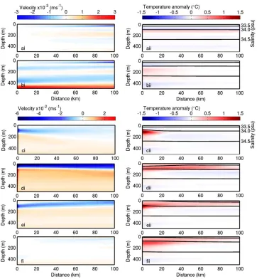
Figure 5 shows the along-fjord velocity patterns produced in these simulations. In the absence of a glacier, there is little movement: only weak currents near the ocean boundary generated by horizontal salinity gra-dients forming in response to gradual vertical diffusion (Figure 5ai). The addition of an ice front, but no runoff, generates a series of vertical circulation cells, driven by melting at the fjord head (Figure 5bi). These currents remain very weak, however, with maximum predicted velocities of the order of 1023m s21. The addition of runoff stimulates a much stronger circulation, with a clear seasonality (Figures 5ci–fi). As runoff increases dur-ing the sprdur-ing, a down-fjord current forms at the depth at which the plume reaches neutral buoyancy, com-pensated by a weaker but thicker up-fjord current below (Figure 5ci). The depth of the down-fjord current decreases and its strength increases as runoff increases, until by peak runoff it occupies the upper100 m of the water column with a maximum velocity of the order of 0.1 m s21(Figure 5di). At this stage, the fjord resembles a single-cell estuarine circulation. The reverse of this process happens during autumn, with the down-fjord current increasing in depth and decreasing in strength as runoff decreases (Figure 5ei).
head, most notably in the lower part of the water column where the warmer waters are cooled by 0.1 to 0.2C (Figure 5bii). A similar cooling occurs in the runoff scenario, but greater change to the temperature structure occurs due to the vertical movement of water within the plume (Figures 5cii– 5fii). In keeping with the results of the plume model experiment (Figure 3), the waters exiting the plume at the depth of neutral buoyancy tend to be warmer than the ambient conditions at that depth, particularly when the plume terminates in the cold band between approximately 80 and 180 m depth. This generates a general warming of the upper part of the water column, with the warmest layer in the upper part of the water column often coinciding with the depth of the down-fjord current at that time (Figure 5).
[image:9.630.203.565.95.487.2]Changes to the salinity distribution in the fjord are less notable (Figures 5aii–5fii). Outflow from the plume inputs a large quantity of water of constant salinity at some depth in the water column. This water may pileup near the ice front, generating a slight along-fjord salinity gradient. As runoff increases and the depth of the plume outflow decreases, the up-fjord currents generated by plume entrainment serve to restore the original salinity distribution.
Figure 5.Fjord centerline sections showing (i) along-fjord velocity (m s21
) and (ii) temperature anomaly (C) with isohalines (psu). The
3.4. Impact of Runoff on Submarine Melt Rate
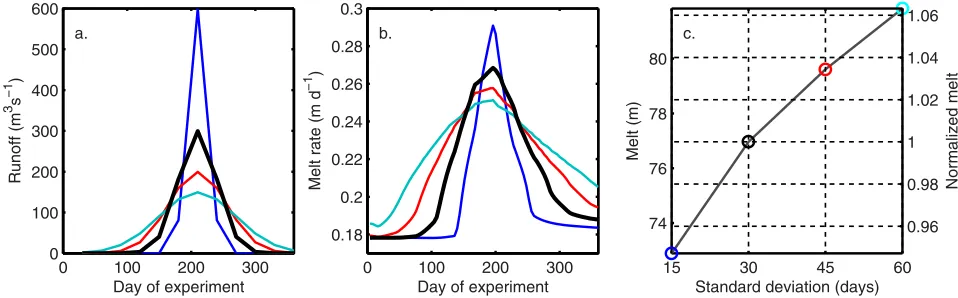
Theoretical and numerical modeling experiments have shown that submarine melt rate increases with the discharge of subglacial runoff from a single channel [e.g.,Jenkins, 2011;Sciascia et al., 2013;Xu et al., 2013, 2012]. However, the significance of this relationship when considered across the entire ice front and on annual and interannual time scales is not well understood. To investigate this, we conducted a series of 1 year experiments in which the magnitude of the summer melt season was varied. Taking the seasonal run-off distribution used in section 3.3 (7 months long, peaking at 300 m3s21in July) as a base case ‘‘standard’’ year, we conducted a series of experiments with total annual runoff scaled to 0.5, 1.5, and 2 times this value, representing a generous allowance for interannual variability. (For comparison,Mernild et al. [2010] estimate interannual variability in total annual runoff from Helheim Glacier to reach a maximum of approximately 625% of the mean over the period 1999–2008.) In the first set of experiments, we achieve this by varying theintensityof melt season, such that its duration remains constant but the magnitude of runoff is scaled accordingly. In the second set of experiments, we keep the peak July runoff at 300 m3s21, and instead vary thedurationof the melt season, maintaining a normal distribution. The resulting runoff time series are shown in Figures 2b and 2c.
As seen in Figure 4, the average ice front melt rate can be broken into two components: ‘‘plume melting,’’ where the plume comes into contact with the glacier, and ‘‘background melting’’ where it does not. The for-mer component scales with discharge, causing average melt rate to rise toward the middle of the melt sea-son then fall again (Figures 6a and 6b). If only the central 200 m of the ice front are considered, plume melting dominates and we find a similar power law relation between melt and discharge to that identified in previous studies [Jenkins, 2011;Sciascia et al., 2013;Xu et al., 2012], withm_ /Q2=5(Figure 6c). However, 0 100 200 300
0.18 0.2 0.22 0.24 0.26 0.28
Day of experiment
Melt rate (md
−1
)
a.
0 100 200 300 0.18 0.2 0.22 0.24 0.26 0.28
Day of experiment
Melt rate (md
−1
)
b.
0 1 2 3
x 109 15
20 25
d.
Runoff (m3)
Melt (m)
0 0.5 1 1.5 2
0.6 0.8 1 1.2 1.4 Normalized runoff Normalized melt u
bg = 0.01 ms −1
0 1 2 3
x 109 60
80 100
Runoff (m3)
Melt (m)
e.
Intensity Duration 0x 0.5x 1x 1.5x 2x
0 0.5 1 1.5 2
0.6 0.8 1 1.2 1.4 Normalized runoff Normalized melt u
bg = 0.06 ms −1
0 1 2 3
x 109 80
100 120 140 160 f.
Runoff (m3)
Melt (m)
0 0.5 1 1.5 2
0.6 0.8 1 1.2 1.4 Normalized runoff Normalized melt u
bg = 0.10 ms −1
0 200 400 600 0
1 2 3
Discharge (m3 s−1)
Melt rate (m d
−1
) c.
Model output
[image:10.630.73.560.101.403.2]Q2/5
Figure 6.Relationships between runoff and submarine melt rate. Seasonal variation in mean melt rate across the ice front with varying (a) runoff intensity and (b) runoff duration, using
a background velocity of 0.06 m s21
. Results calculated with alternative background velocities are shown in the supporting information. (c) Seasonal relationship between runoff and melt rate for the central 200 m of the ice front (containing the plume), throughout the 23runoff intensity experiment. Dots show the value every 4 days, while the red line shows the trendline withm_ / Q2=5. Relationship between total annual runoff and total annual melt (m water equivalent, averaged across the ice front), using a background velocity of (d) 0.01 m
s21
, (e) 0.06 m s21
, and (f) 0.10 m s21
when the entire width of the ice front is considered, the background melt rate becomes much more signifi-cant. As in Figure 4, we do not find that the plume generates sufficient cross-fjord circulation to strongly influence this background melt rate, although the existence of relatively warm glacially modified waters leads to a slightly higher melt rate in the autumn relative to spring (Figures 6a and 6b). Instead, we find that the background melt rate is strongly dependent on the minimum velocity value prescribed in equation (6) (see also supporting information). This is problematic, as this value remains somewhat artificial and is diffi-cult to constrain.
[image:11.630.75.554.100.249.2]Increasing the intensity of runoff results in higher peak summer melt rates (Figures 6a and 6b). However, as identified here (Figure 6c) and in previous studies [Jenkins, 2011;Sciascia et al., 2013;Xu et al., 2012], the sen-sitivity of plume melt rate to discharge decreases as discharge rises (Figure 6c), meaning the difference between scenarios is somewhat subdued. For example, doubling peak runoff from 300 to 600 m3s21results in a25% increase in peak melt rate relative to the background melt rate (Figure 6a). Increasing the dura-tion of the melt season has a greater effect for the same increase in annual runoff, because plume melt rate is more sensitive to variation in discharge at lower discharge values (Figure 6c). This effect can be seen most clearly when the duration of the melt season is altered while the total annual runoff is kept constant (Figure 7). Although the more intense melt seasons generate higher peak melt rates, this is more than com-pensated by the greater duration of enhanced melt rates in the longer melt seasons (Figure 7).
The significance of annual and interannual variability in runoff on total melt rate depends on the back-ground melt rate, which in turn depends on the prescribed backback-ground velocity (Figures 6d–6f). In the sce-nario with the smallest background melt rate (Figure 6d), doubling total runoff from the standard scesce-nario results in a15–45% increase in total annual melting. In the moderate background melt rate scenario, this drops to a 3–12% increase (Figure 6e), while in the highest background melt rate scenario, this falls further to 2–8% (Figure 6f). This behavior is discussed further in section 4.
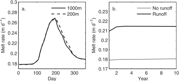
Following this, the model was run for 10 consecutive years to examine whether there was a cumulative impact on melt rate over this time (for example, due to a sustained cooling near the ice front). Two scenar-ios were run—in the first, there was no runoff; in the second, the standard runoff forcing was repeated for 10 cycles. In order to reduce the computational time required, the horizontal model resolution was increased to a uniform 1000 m in along and across-fjord directions. The effect of this coarser resolution is assessed in Figure 8a, which shows the submarine melt rate over the course of 1 year, as predicted using the original horizontal model resolution and the coarser grid. During the first part of the year, the predicted melt rates in the two simulations are almost identical, while in the second part of the year, the predicted melt rate is slightly reduced in the coarser domain. The overall similarity of results demonstrates the impor-tance of the plume melting (which is independent of the model resolution) on the total melt rate and justi-fies the use of the coarser-resolution domain for these experiments (see also supporting information). The 0 100 200 300
0 100 200 300 400 500 600
Day of experiment
Runoff (m
3 s
−1
)
a.
0 100 200 300 0.18
0.2 0.22 0.24 0.26 0.28 0.3
Day of experiment
Melt rate (m d
−1
)
b.
15 30 45 60
74 76 78 80
Melt (m)
Standard deviation (days) c.
0.96 0.98 1 1.02 1.04 1.06
Normalized melt
Figure 7.Effect on melt rate of modifying the duration of seasonal runoff while keeping total seasonal runoff constant. (a) Runoff forcing used in each experiment. The thick black line
results of the 10 year simulations are shown in Figure 8b. There is a small increase in melt rate following the first year in the standard runoff scenario due to the displacement of cold water from adjacent to the glacier by warmer glacially modified water. With the exception of this, there is however little change in melt rate in either scenario over the 10 years. This suggests that, with or without runoff, there is no significant cumula-tive cooling or warming of the fjord waters surrounding the glacier front on this time scale (assuming no other external change in properties of the fjord water entering the fjord mouth).
4. Discussion
4.1. Glacial Modification of Fjord Oceanography
Oceanographic survey data from Greenland’s fjords are sparse and frequently limited to late summer when ice cover in the fjords is at its annual minimum. The area close to the ice front, often choked with icebergs and sea ice and at risk from calving events, is extremely difficult to survey, making data from this crucial location in which glacially modified water masses are formed particularly rare [Straneo et al., 2013]. This makes interpretation of existing data sets and model results challenging, limiting our understanding of the impact of glaciers on fjord oceanography.
Nevertheless, several authors have used temperature and salinity characteristics to argue for the existence of glacially modified layers in fjord survey data. At Sermilik Fjord, east Greenland,Straneo et al. [2011] identi-fied a relatively warm layer extending over 50 km from the ice front at a depth of between 100 and 200 m. They argued that this layer was formed by subglacial runoff and entrained warm Atlantic waters, rising upward until it reached neutral buoyancy at the steep halocline between the Atlantic waters and the overly-ing cooler, fresher Polar waters. Similarly at Store Glacier,Chauche et al. [2014] reported the presence of warm, glacially modified layers in the upper part of the water column. In August 2010, this layer occurred at the surface, above the coldest water, while during the cooler August of 2009 the glacially modified waters were found both at the surface and lower in the water column. This occurred, they argued, because reduced runoff meant that the plume reached neutral buoyancy lower in the water column during the cooler year.
Our findings support and add further detail to these hypotheses. We find that as runoff increases through the spring, the plume grows in strength and rises higher in the water column. As it does so, the waters near the ice front are replaced with a mixture of entrained fjord waters, glacial runoff, and the products of sub-marine melt. Of these, the fjord waters are dominant and the subsub-marine meltwater is negligible. For exam-ple, by the point of neutral buoyancy in the highest discharge scenario in Figure 3, the plume is
transporting>6000 m3s21of entrained fjord water, 100 m3s21of glacial runoff, and 1.5 m3s21of fresh-water from submarine melting. If the fjord was vertically uniform in temperature, this mixture would be slightly cooler than the ambient waters. However, because deep silled Greenlandic fjords are characterized by a warmer, saltier layer of Atlantic waters underlying a cooler, fresher layer of Polar waters [Straneo and
0 100 200 300 0.18
0.2 0.22 0.24 0.26 0.28 0.3
Day
Melt rate (m d
−1
)
a.
2 4 6 8 10
0.17 0.18 0.19 0.2 0.21 0.22 0.23
Year
Melt rate (m d
−1
)
b. 1000m
200m
[image:12.630.234.536.101.237.2]No runoff Runoff
Figure 8.(a) Mean ice front melt rate over a 1 year experiment with standard runoff forcing, conducted using the original horizontal
Heimbach, 2013], this glacially modified water is typically warmer than the ambient waters at the depth at which it reaches neutral buoyancy.
The plume outflow sets up a circulatory cell, with a thinner, stronger down-fjord current overlying a thicker, weaker, up-fjord current. Maximum modeled along-fjord velocities are on the order of 0.01–0.1 m s21, in agreement with the residual runoff-driven circulation identified bySutherland and Straneo[2012] in Sermilik Fjord, east Greenland. Glacially modified waters are reentrained by this cell as the outlet point of the plume rises during the spring, and so in summer there may be little evidence of this modification below the depth of the main plume outflow (e.g., Figure 5d). This is likely to be the scenario observed byChauche et al. [2014] during August 2010, when the only runoff-modified waters are in the surface layer. As runoff decreases in the autumn, the plume loses strength and drops down through the water column again (Fig-ure 5e). Glacially modified waters become trapped in the relatively slow flowing zone above the level of the main circulatory cell as the depth of the down-fjord current increases during this phase. These glacially modified waters may form a warm zone around the glacier front, as observed byChauche et al. [2014] dur-ing August 2009.
Not all fjord survey data fit this picture. In Kangerdlugssuaq Fjord, east Greenland,Inall et al. [2014] report cold glacially modified waters, while warm surface waters originate on the shelf, the opposite of the sce-nario reported at Store Glacier [Chauche et al., 2014]. This may be because an extensive ice melange exists in front of Kangerdlugssuaq Glacier, acting as a substantial additional heat sink [Enderlin and Hamilton, 2014]. This demonstrates the complexity of the glacial fjord system, with multiple freshwater inputs (includ-ing subglacial and surface runoff, as well as meltwater from icebergs and glaciers) interact(includ-ing with complex and evolving water masses originating beyond the fjord mouth. In this study, we are focusing on a simpli-fied system, in which only subglacial runoff and melting from a single glacier act upon the fjord. As such, the features that we identify here will in reality be but one component of more complex and variable circu-lation [Sutherland and Straneo, 2012].
A further level of complexity that may be present in real-world scenarios is across-fjord variability in circula-tion and fjord water properties, introduced by both topographic complexity and the effects of rotacircula-tion. The Rossby radius of deformation of our idealized fjord is9 km, which is large compared to the fjord width of 5 km (Kelvin number50.55) [Garvine, 1995]. As such, the modeled fjord is dynamically narrow and rotation is not important. Large Greenlandic fjords such as Sermilik Fjord and Kangerdlugssuaq Fjord are typically slightly wider than the 5 km width used here, and the Kelvin number can equal or exceed unity in places [Sutherland et al., 2014].Sutherland et al. [2014] find geostrophic currents to be of importance offshore of the fjord mouths, but report only limited evidence of lateral gradients within the fjords themselves. Con-trastingly,Inall et al. [2014] report significant across-fjord gradients midway along Kangerdlugssuaq Fjord, arguing that circulation within the fjord is in geostrophic balance. It is therefore possible that in Greenland’s largest (and in particular broadest) fjords, rotation may become significant, generating greater across-fjord variation in circulation patterns than is apparent in the experiments undertaken here (supporting
information).
4.2. Interaction of Runoff, Fjord Circulation, and Submarine Melt Rate
There are several ways in which variability in runoff could influence glacier melt rate. The first, as investi-gated in previous studies [e.g.,Jenkins, 2011;Xu et al., 2012], is that increased runoff generates a more vigor-ous upwelling, and as such generates higher melt rates where this plume comes into contact with the ice front. The second mechanism would be if this plume generated stronger currents across a wider part of the ice front, causing an increase in melt rate extending beyond the area in contact with the plume. The third mechanism is that the along-fjord circulation driven by the runoff could help to supply warm water to the fjord head.
scenario (Figure 5). A similar cooling at depth close to the ice front is observed in the runoff and no-runoff scenarios even after 10 years, although there is a modest (<3%) increase in melt rate in the runoff scenario due to the displacement of cold water masses in the upper part of the water column by glacially modified waters (Figure 8). This situation may be different if the temperature of the water mass at the fjord mouth changed over time, as the glacially forced circulation could serve to accelerate the rate at which these changes affected the properties of the water in contact with the glacier. Further work is required to address this uncertainty, in particular examining the relative importance of glacially and coastally forced fjord shelf exchange in a range of geographical settings [e.g.,Jackson et al., 2014;Sciascia et al., 2014;Sutherland et al., 2014].
The cumulative effect of these processes is that average melt rate increases in the summer due to more rapid melting where the ice is in contact with the plume and remains slightly elevated the following winter due to the displacement of cold water masses (Figure 6). Whether or not these processes result in a signifi-cant increase in the total mass loss through submarine melting depends on the background melt rate, which remains comparatively steady across large sections of the ice front over the course of the year. Melt rate is strongly dependent on the velocity at the ice-ocean interface [Jenkins et al., 2010], and so cannot be properly predicted without knowledge of these currents (supporting information). However, resolving buoy-ant convection due to melting on this boundary would require an extremely fine mesh in this zone, which is computationally impractical. It may be possible to include this process through the use of an additional coupled model similar to our parameterization of the main runoff-forced plume, but this would require the development of an appropriate melt-driven convection model, which lies beyond the scope of this paper. Alternatively, a simple parameterization based on observation of submarine melt rates at tidewater glaciers would be invaluable, but obtaining the data required to formulate such a parameterization remains extremely challenging in this hostile environment [Straneo et al., 2013].
If the background melt rate is in reality very low, then variability in runoff may be responsible for large rela-tive changes in melt rate (Figure 6d). However, it is difficult to reconcile low overall melt rates with those derived from field-based heat flux estimates which place typical submarine melt rates at Greenland’s gla-ciers in the range of1–10 m d21[Inall et al., 2014;Rignot et al., 2010;Sutherland and Straneo, 2012], which
would imply melt rate away from the main plume is high and contributes significantly to the total melt rate. If this is the case, then runoff variability, particularly on the scale of interannual variability, may not result in substantial variability in submarine melt rate. There are however large uncertainties in the melt calculations used in both modeling and observational studies. The melt parameterizations used here and in other mod-els of submarine melting [Sciascia et al., 2013;Xu et al., 2013, 2012] remain poorly validated for the vertical faces and strong currents of tidewater glacier fronts, having been developed and tested based on heat transfers beneath ice shelves and sea ice [Holland and Jenkins, 1999]. Field-based melt rate estimations [Inall et al., 2014;Rignot et al., 2010;Sutherland and Straneo, 2012] on the other hand, are often based on heat flux estimates from relatively sparse observations acquired at some distance from the ice front, and do not account for the potentially considerable loss of heat through melting of the ice melange [Enderlin and Ham-ilton, 2014]. As such, comparing field and model-based melt rate estimates remains problematic.
A further consideration is that runoff may not be concentrated into a single large channel when it enters the fjord. Although field observations seldom report more than one large plume [e.g.,Chauche et al., 2014;
Sole et al., 2011], there may be numerous smaller plumes that never reach the fjord surface and so remain undetected. If runoff is shared between several smaller channels rather than (or in addition to) emerging from a single main source, the individual plumes will be weaker, and so the melting associated with each individual plume smaller. Nevertheless, average melt rate across the entire ice front may be increased as a greater proportion of the ice is affected by plumes [Kimura et al., 2014]. The basis of this result lies in the sublinear relationship between freshwater discharge and average plume melt rate, with melting scaling with discharge raised to the power of1/3 to 1/2 [Jenkins, 2011;Sciascia et al., 2013;Xu et al., 2012]. This means that for a given total runoff, concentrating this runoff leads to a decrease in total melting. This rea-soning also applies with respect to time, with a longer melt season generating greater total melting for a given total runoff (Figure 7).
drainage system may persist during the winter months (fed by basal frictional melting), reducing seasonal variability in submarine melt rate. It is clear that a more complete understanding of tidewater glacier hydrol-ogy is required to better constrain submarine melt rate, and how this varies in space and time [Straneo et al., 2013].
A further factor that is likely to be important in this respect is the feedback between submarine melting and calving as the morphology of the calving front is modified by spatially uneven melting [O’Leary and Christof-fersen, 2013]. If submarine melt is concentrated around a large channel then this may cut back into the gla-cier, causing enhanced calving in the surrounding region that spreads out across the ice front [Chauche et al., 2014]. Alternatively, if runoff is more widely distributed across the grounding line, greater melting at depth may undercut the ice front [O’Leary and Christoffersen, 2013]. Better understanding of the links between submarine melting and calving mechanics is therefore necessary in order to assess whether the average ice front melt rate, or the spatial distribution of submarine melting, is more important in controlling tidewater glacier mass balance.
4.3. Comparison With Previous Numerical Modeling Studies
This paper represents a first attempt to model the impact of glacial runoff on fjord oceanography by cou-pling a theoretical plume routine to an ocean circulation model. In recent years however, several studies have used MITgcm to model the formation of plumes arising from subglacial discharge by using a high-resolution set up in which the plume turbulence is partially resolved [Sciascia et al., 2013;Xu et al., 2013, 2012]. Several key elements are consistent between this study, previous numerical modeling studies and field surveys: subglacial runoff generates a plume that rises adjacent to the glacier, producing a glacially modified down-fjord current underlain by an up-fjord current. One feature of field surveys that modeling studies have sought to reproduce is the observation that glacially modified currents may form at an inter-mediate depth between the surface and bed [Chauche et al., 2014;Straneo et al., 2011], in contrast to a clas-sic estuarine circulation in which the outflow occurs at the surface [e.g.,Motyka et al., 2013]. While previous modeling studies have succeeded in generating glacial plumes which reach neutral buoyancy and flow down-fjord at some intermediate depth, this has only occurred at discharges less than5 m3s21[Sciascia et al., 2013;Xu et al., 2012] to30 m3s21[Xu et al., 2013]. These values are very low compared to the expected summer runoff from these glaciers (hundreds of cubic meters per second), indicating that runoff-modified waters should be present at the surface throughout much of the year.
In the case ofXu et al. [2012] andSciascia et al. [2013], this discrepancy occurs principally because the domains used in these earlier studies were two dimensional. This means that the surface area across which fjord water can be entrained into the plume is greatly reduced (i.e., there is no entrainment in an across-fjord direction), allowing the plume to remain buoyant higher into the water column. This case is similar to the plume model ofJenkins[2011], in which entrainment is only permitted on the down-fjord face of the plume, allowing the plume to rise higher into the water column relative to the half-conical plume geometry that we employ in this study (Figure 3).
5. Conclusions
In this paper, we have used a plume model to parameterize the buoyant upwelling of subglacial runoff in an ocean circulation model. This greatly improves the computational efficiency of modeling glacial fjords, permitting simulation of larger domains (hundreds of square kilometers in area) over longer time periods (years to decades) than has previously been possible. This model has been used to examine the effect of runoff on fjord circulation and submarine melt rate independent of coastal forcing. In these simulations, runoff generates a relatively thin, strong, down-fjord current overlying a relatively thick, slow up-fjord cur-rent. The strength and depth of the down-fjord current varies with runoff on annual time scales, being strongest, and forming highest in the water column, when runoff is greatest. Because this current contains entrained Atlantic waters from the lower part of the water column, it is typically warmer than the ambient conditions at the depth at which it forms. This finding supports the identification of anomalously warm, gla-cially modified waters in some Greenlandic fjords [Chauche et al., 2014;Straneo et al., 2011].
Submarine melt rate increases strongly with runoff in areas where ice is in contact with a buoyant runoff-driven plume. This contact area may be small however relative to the width of the tidewater glacier margin, and the impact is greatly reduced when averaged across the entire ice front. We find the submarine melt rate to be only weakly sensitive to runoff when considered on the scale of interannual variability and across the full width of the glacier. The significance of the relationship between runoff and submarine melt rate is however dependent on the distribution of runoff across the grounding line and the strength of the back-ground melt rate in those areas not in contact with the plume, both of which remain poorly constrained. In recent years, there has been much interest in the relationship between melt rate and discharge in the vicin-ity of ice marginal plumes [e.g.,Jenkins, 2011;Sciascia et al., 2013;Xu et al., 2013]; further work is needed to better constrain both the proportion of the ice front directly affected by runoff-driven plumes and the sub-marine melt rate across the remainder in order to improve the prediction of melt rate across the full width of the glacier front. Furthermore, this must be combined with a better knowledge of how the rate and distri-bution of melting influences calving mechanics before the significance of submarine melting for the mass balance of tidewater glaciers can be accurately assessed.
References
Adcroft, A., C. Hill, J. M. Campin, J. Marshall, and P. Heimbach (2004), Overview of the formulation and numerics of the MIT GCM, in Proceed-ings of the ECMWF Seminar Series on Numerical Methods, Recent Developments in Numerical Methods for Atmosphere and Ocean Model-ling, pp. 139–149. [Available at http://old.ecmwf.int/publications/library/do/references/list/17334.]
Campin, J.-M., and H. Goosse (1999), Parameterization of density-driven downsloping flow for a coarse-resolution ocean model in z-coordi-nate,Tellus, Ser. A,51(3), 412–430.
Chauche, N., A. Hubbard, J. C. Gascard, J. E. Box, R. Bates, M. Koppes, A. Sole, P. Christoffersen, and H. Patton (2014), Ice-ocean interaction and calving front morphology at two west Greenland tidewater outlet glaciers,Cryosphere,8(4), 1457–1468.
Enderlin, E. M., and G. S. Hamilton (2014), Estimates of iceberg submarine melting from high-resolution digital elevation models: Applica-tion to Sermilik Fjord, East Greenland,J. Glaciol.,60(224), 1084–1092.
Garvine, R. W. (1995), A dynamical system for classifying buoyant coastal discharges,Cont. Shelf Res.,15(13), 1585–1596, doi:10.1016/0278– 4343(94)00065-u.
Heimbach, P., and M. Losch (2012), Adjoint sensitivities of sub-ice-shelf melt rates to ocean circulation under the Pine Island Ice Shelf, West Antarctica,Ann. Glaciol.,53(60), 59–69, doi:10.3189/2012/AoG60A025.
Hindmarsh, A. C. (1983), ODEPACK, a systemized collection of ODE solvers, inScientific Computing, edited by R. S. Stepleman, pp. 55–64, North-Holland Publishing Company, Amsterdam.
Holland, D. M., and A. Jenkins (1999), Modeling thermodynamic ice-ocean interactions at the base of an ice shelf,J. Phys. Oceanogr.,29(8), 1787–1800, doi:10.1175/1520-0485(1999)029<1787:mtioia>2.0.co;2.
Holland, D. M., R. H. Thomas, B. De Young, M. H. Ribergaard, and B. Lyberth (2008), Acceleration of Jakobshavn Isbrae triggered by warm subsurface ocean waters,Nat. Geosci.,1(10), 659–664, doi:10.1038/ngeo316.
Huppert, H. E., and E. G. Josberger (1980), The melting of ice in cold stratified water,J. Phys. Oceanogr.,10(6), 953–960, doi:10.1175/1520-0485(1980)010<0953:tmoiic>2.0.co;2.
Inall, M. E., T. Murray, F. R. Cottier, K. Scharrer, T. J. Boyd, K. J. Heywood, and S. L. Bevan (2014), Oceanic heat delivery via Kangerdlugssuaq Fjord to the south-east Greenland ice sheet,J. Geophys. Res. Oceans,119, 631–645, doi:10.1002/2013JC009295.
Jackett, D. R., and T. J. McDougall (1995), Minimal adjust of hydrographic profiles to achieve static stability,J. Atmos. Oceanic Technol., 12(2), 381–389, doi:10.1175/1520-0426(1995)012<0381:maohpt>2.0.co;2.
Jackson, R. H., F. Straneo, and D. A. Sutherland (2014), Externally forced fluctuations in ocean temperature at Greenland glaciers in non-summer months,Nat. Geosci.,7(7), 503–508, doi:10.1038/ngeo2186.
Jacobs, S. S., H. E. Huppert, G. Holdsworth, and D. J. Drewry (1981), Thermohaline steps induced by melting of the Erebus Glacier tongue,J. Geophys. Res.,86(C7), 6547–6555, doi:10.1029/JC086iC07p06547.
Jenkins, A. (2011), Convection-driven melting near the grounding lines of ice shelves and tidewater glaciers,J. Phys. Oceanogr.,41(12), 2279–2294, doi:10.1175/jpo-d-11-03.1.
Jenkins, A., K. W. Nicholls, and H. F. J. Corr (2010), Observation and parameterization of ablation at the base of Ronne Ice Shelf, Antarctica, J. Phys. Oceanogr.,40(10), 2298–2312, doi:10.1175/2010jpo4317.1.
Acknowledgments
Kantha, L. H., and C. A. Clayson (2000),Numerical Models of Oceans and Ocean Circulation, 750 pp., Academic, San Diego, Calif. Kaye, N. B. (2008), Turbulent plumes in stratified environments: A review of recent work,Atmos. Ocean,46(4), 433–441, doi:10.3137/
ao923.2008.
Kimura, S., P. Holland, and A. Jenkins (2014), The effect of meltwater plumes on the melting of a vertical glacier face,J. Phys. Oceanogr.,44, 3099–3117.
Losch, M. (2008), Modeling ice shelf cavities in azcoordinate ocean general circulation model,J. Geophys. Res.,113, C08043, doi:10.1029/ 2007JC004368.
Marshall, J., A. Adcroft, C. Hill, L. Perelman, and C. Heisey (1997a), A finite-volume, incompressible Navier Stokes model for studies of the ocean on parallel computers,J. Geophys. Res.,102(C3), 5753–5766, doi:10.1029/96JC02775.
Marshall, J., C. Hill, L. Perelman, and A. Adcroft (1997b), Hydrostatic, quasi-hydrostatic, and nonhydrostatic ocean modeling,J. Geophys. Res.,102(C3), 5733–5752, doi:10.1029/96JC02776.
Mernild, S. H., and G. E. Liston (2012), Greenland freshwater runoff. Part II: Distribution and trends, 1960–2010,J. Clim.,25(17), 6015–6035, doi:10.1175/jcli-d-11–00592.1.
Mernild, S. H., I. M. Howat, Y. Ahn, G. E. Liston, K. Steffen, B. H. Jakobsen, B. Hasholt, B. Fog, and D. van As (2010), Freshwater flux to Sermilik Fjord, SE Greenland,Cryosphere,4(4), 453–465, doi:10.5194/tc-4–453-2010.
Mortensen, J., K. Lennert, J. Bendtsen, and S. Rysgaard (2011), Heat sources for glacial melt in a sub-Arctic fjord (Godthabsfjord) in contact with the Greenland Ice Sheet,J. Geophys. Res.,116, C01013, doi:10.1029/2010JC006528.
Morton, B., G. Taylor, and J. Taylor (1956), Turbulent gravitational convection from maintained and instantaneous sources,Proc. R. Soc. Lon-don, Ser. A,234(1196), 1–23, doi:10.1098/rspa.1956.0011.
Motyka, R. J., W. P. Dryer, J. Amundson, M. Truffer, and M. Fahnestock (2013), Rapid submarine melting driven by subglacial discharge, LeConte Glacier, Alaska,Geophys. Res. Lett.,40, 5153–5158, doi:10.1002/grl.51011.
O’Leary, M., and P. Christoffersen (2013), Calving on tidewater glaciers amplified by submarine frontal melting,Cryosphere,7(1), 119–128. Paluszkiewicz, T., and R. D. Romea (1997), A one-dimensional model for the parameterization of deep convection in the ocean,Dyn. Atmos.
Oceans,26(2), 95–130, doi:10.1016/s0377-0265(96)00482-4.
Price, J., and J. Yang (1998), Marginal sea overflows for climate simulations, inOcean Modeling and Parameterization, edited by E. Chas-signet and J. Verron, pp. 155–170, Kluwer Academic Publishers, Dordrecht, Netherlands.
Rignot, E., M. Koppes, and I. Velicogna (2010), Rapid submarine melting of the calving faces of West Greenland glaciers,Nat. Geosci.,3(3), 187–191, doi:10.1038/ngeo765.
Salcedo-Castro, J., D. Bourgault, and B. de Young (2011), Circulation induced by subglacial discharge in glacial fjords: Results from idealized numerical simulations,Cont. Shelf Res.,31(13), 1396–1406, doi:10.1016/j.csr.2011.06.002.
Sciascia, R., F. Straneo, C. Cenedese, and P. Heimbach (2013), Seasonal variability of submarine melt rate and circulation in an East Green-land fjord,J. Geophys. Res. Oceans,118, 2492–2506, doi:10.1002/jgrc.20142.
Sciascia, R., C. Cenedese, D. Nicoli, P. Heimbach, and F. Straneo (2014), Impact of periodic intermediary flows on submarine melting of a Greenland glacier,J. Geophys. Res. Oceans,119, 7078–7098, doi:10.1002/2014JC009953.
Sole, A. J., D. W. F. Mair, P. W. Nienow, I. D. Bartholomew, M. A. King, M. J. Burke, and I. Joughin (2011), Seasonal speedup of a Greenland marine-terminating outlet glacier forced by surface melt-induced changes in subglacial hydrology,J. Geophys. Res.,116, F03014, doi: 10.1029/2010JF001948.
Straneo, F., and C. Cenedese (2015), The dynamics of Greenland’s glacial fjords and their role in climate,Ann. Rev. Mar. Sci.,7, 1–24. Straneo, F., and P. Heimbach (2013), North Atlantic warming and the retreat of Greenland’s outlet glaciers,Nature,504(7478), 36–43, doi:
10.1038/nature12854.
Straneo, F., G. S. Hamilton, D. A. Sutherland, L. A. Stearns, F. Davidson, M. O. Hammill, G. B. Stenson, and A. Rosing-Asvid (2010), Rapid circu-lation of warm subtropical waters in a major glacial fjord in East Greenland,Nat. Geosci.,3(3), 182–186, doi:10.1038/ngeo764. Straneo, F., R. G. Curry, D. A. Sutherland, G. S. Hamilton, C. Cenedese, K. Vage, and L. A. Stearns (2011), Impact of fjord dynamics and glacial
runoff on the circulation near Helheim Glacier,Nat. Geosci.,4(5), 322–327, doi:10.1038/ngeo1109.
Straneo, F., et al. (2013), Challenges to understanding the dynamic response of Greenland’s marine terminating glaciers to oceanic and atmospheric forcing,Bull. Am. Meteorol. Soc.,94(8), 1131–1144, doi:10.1175/bams-d-12–00100.1.
Sutherland, D. A., and F. Straneo (2012), Estimating ocean heat transports and submarine melt rates in Sermilik Fjord, Greenland, using low-ered acoustic Doppler current profiler (LADCP) velocity profiles,Ann. Glaciol.,53(60), 50–58, doi:10.3189/2012AoG60A050.
Sutherland, D. A., F. Straneo, and R. S. Pickart (2014), Characteristics and dynamics of two major Greenland glacial fjords,J. Geophys. Res. Oceans,119, 3767–3791, doi:10.1002/2013JC009786.
Tedstone, A. J., and N. S. Arnold (2012), Automated remote sensing of sediment plumes for identification of runoff from the Greenland ice sheet,J. Glaciol.,58(210), 699–712, doi:10.3189/2012JoG11J204.
Wells, A. J., and M. G. Worster (2008), A geophysical-scale model of vertical natural convection boundary layers,J. Fluid Mech.,609, 111– 137, doi:10.1017/s0022112008002346.
Xu, Y., E. Rignot, D. Menemenlis, and M. Koppes (2012), Numerical experiments on subaqueous melting of Greenland tidewater glaciers in response to ocean warming and enhanced subglacial discharge,Ann. Glaciol.,53(60), 229–234, doi:10.3189/2012AoG60A139. Xu, Y., E. Rignot, I. Fenty, D. Menemenlis, and M. M. Flexas (2013), Subaqueous melting of Store Glacier, west Greenland from
![Figure 2. Initial conditions and forcings used in the model experiments. (a) Temperature and salinity profiles used as initial conditions, derived by averaging Store Fjord profiles takenduring August 2010 [Chauch�e et al., 2014]](https://thumb-us.123doks.com/thumbv2/123dok_us/7876767.183166/5.630.75.559.102.263/conditions-experiments-temperature-proles-conditions-averaging-proles-takenduring.webp)
![Figure 3. Results generated using the plume model with a freshwater input of 1, 10, and 100 m[2011] using freshwater inputs of 10 and 100 m3 s21 (blue)](https://thumb-us.123doks.com/thumbv2/123dok_us/7876767.183166/6.630.74.558.101.443/figure-results-generated-using-plume-freshwater-freshwater-inputs.webp)