The CQDRNG8 - a quadratic, isoparametric, axisymmetric finite element for the NASTRAN computer program

1977

The CQDRNG8 - a quadratic, isoparametric,

axisymmetric finite element for the NASTRAN

computer program

John Gray

Follow this and additional works at:

http://scholarworks.rit.edu/theses

This Thesis is brought to you for free and open access by the Thesis/Dissertation Collections at RIT Scholar Works. It has been accepted for inclusion in Theses by an authorized administrator of RIT Scholar Works. For more information, please [email protected].

Recommended Citation

Approved by:

John F. Gray

A Thesis Submitted

in

Partial Fulfillment

of the

Requirements for the Degree of

MASTER OF SCIENCE

in

Mechanical Engineering

Prof.

Prof.

Wayne Walters

B. Karlekar

Prof. ____

~N~e~v~i~lIe~R~ie~g~e~r

____ _

Prof. ____

R_ic_h_a~r~d~B_.~H~e~tn~a~r~sk~i

__ _

DEPARTl'-1ENT OF MECHAJ.1I CAL

Ei~G

IN EE-RING

ROCHESTER INSTITUTE OF TECHNOLOGY

ROCHESTER, NEW YORK

The success of this _undertaking is

largely

due to the cooperation

of _many persons. I would like to express _my deepest gratitude to the

following:

To _my wife Phyllis and _my son Kevin for their patience and under

standing throughout this time period.

To Dr. V.

Genberg

and Mr. P.

Mueller,

Eastman Kodak

Company,

for their suggestions and technical advice.

To S.

Wall,

J.

Joseph,

and R.

Harder,

The MacNeal-Schwendler

Corporation,

for their gracious assistance in _providing needed insight

into the MSC/NASTRAN program.

To Professors W.

Walter,

my thesis adviser, and N.

Rieger,

Rochester

Institute of

Technology,

Mechanical

Engineering

Department,

for their

guidance and suggestions.

To Eastman Kodak

Company

for use of the computer facilities and

MSC/NASTRAN finite element program are given. The element is an

eight-noded isoparametric quadrilateral of quadratic order. The

following

matrices and capabilities are developed:

*

1. stiffness matrix for homogeneous isotropic materials,

2. thermal conductance matrix for homogeneous isotropic _materials,

3. calculation of equivalent nodal forces due to temperature

loads,

k.

calculation of _stresses, and

5 _plotting of undeformed and deformed structures.

Several classical thermal and structural problems are solved to

demonstrate these capabilities. In all _cases, the element results

compare well with theory. Comparisons are made to _{existing MSC/NASTRAN}

axisymmetric finite elements. The new element shows _{increased accuracy}

compared to _{the existing} elements. Convergence of the element is

Nomenclature iii

I. Introduction 1

II. Literature Review

3

III. Axisymmetric Structures

7

IV. Element Derivations

9

A. Stiffness Matrix

9

B. Thermoelastic Loads

17

C. Stress

Recovery

19

D. Conductance Matrix 21

V. Additions to NASTRAN

25

VI. Example Problems JO

A.

Bending

of

Simply

Supported Flat Plate J2

B. Thermal Expansion of Circular Disk

39

C. Thermal Expansion of Hollow Sphere

43

D. Heat Flow in a Circular Disk

47

E. Heat Flow in an Axial Rod

57

F. Heat Flow in a Hollow Sphere

59

G. Thermoelastic Stresses in a Hollow Cylinder 64

VII.

Summary

68

VIII. References 72

IX. Appendix A

75

2 Gaussian integration and stress points 20

3

Stiffness matrix partitions 28

4

Deflections of _simply supported plate

33

with center load

5

Deflections of _simply supported plate

35

with concentric circular load

6

Stresses _{in simply} supported plate

37

with load on concentric circle

7

Plot of circular disk model

40

8 Deflections of disk with center hole -

4l

uniform temperature change

9

Plot of hollow sphere model

44

10 Thermal expansion of sphere

45

11 Circular disk models - CQDRNG8 _elements

49

12 Circular disk models - CTRIARG _elements 52

13

Circular disk temperatures

-55

Convergence test

14 Temperatures in axial rod - 58

enforced end temperatures

15

Temperatures in hollow sphere - 60

enforced temperatures at surfaces

16 Temperatures in hollow sphere - 62

enforced temperature at ID

-convection at OD

2 Deflection of _simply supported circular plate J6

with load on concentric circle

3

Stresses _{in simply} supported circular plate 3^

with concentric

loading

4

Thermal deflections in disk

42

5

Thermal expansion of hollow sphere

46

6

Circular disk temperatures - _convergence test 56

7

Temperatures in hollow sphere -

61

enforced temperatures at surfaces

8 Temperatures in hollow sphere

-63

enforced temperature at ID - _{convection at} OD

9

Stresses in hollow cylinder

66

ar'fl'a Normal stresses in r,6,z directions and _shearing

x stress in rz plane

rz r

e >e >e Normal strains in r,9,z directions and _shearing

v strain in rz plane

'rz r

E Young's modulus

v Poisson

's

ratio

VOL Volume

u,v Radial and axial displacement components

N-_

Shape function associated with node i

a>3 Local element coordinates

U Thermal potential function

q Heat flux

density

k Thermal _conductivity

x^ Generalized coordinate

I >

_Vector

[ ]

Matrix

L

J

Inverse of a matrix

IT

{

}

,L

J

Transpose of vector or matrix

I

Determinant of a matrix

LkJ

Stiffness or conductance matrix

(

u

i

Nodal vector of unknowns

(displacements

or

temperatures)

(p)

Nodal vector of applied loads

i

o

}

Element stress vector

{

}

Element strain vector

]

Wj* Gaussian integration _weighting factor

is the absence of a higher order quadrilateral axisymmetric _ring element.

The objective of this thesis is to fill this void. A suitable element

with limited capabilities was developed

by

Janucik. This effort is an

extension of that development. Additional capabilities are developed

and this element is implemented in the NASTRAN program as a DUMMY element.

This _element, named the

CQDRNG8,

_{has many} capabilities. Elastic

stiffness is calculated for homogeneous isotropic materials. Thermo

elastic

loading

is supported. Plots for both undeformed and deformed

structures can be obtained. Element stresses are ouput at the centroid

and the four corner grids of each element. Stress invariants calculated

include the principal stresses and

directions,

the maximum shear, and

the octahedral shear. A thermal conductance matrix is calculated for

homogeneous isotropic materials thus _providing a steady state heat trans

fer capability. The C(^DRNG8 is an eight noded isoparametric quadrilateral

element which allows quadratic variation of displacement and temperature

within the element. A number of user options exist with respect to

both NASTRAN and this element.

The CQDRNG8 element's capabilities are illustrated

by

_solving several

classical thermal and structural problems. In all cases, very good

correlation is observed between theoretical and finite element solutions.

Convergence of the solution for

increasingly

detailed finite element

are those

by

Zienkiewicz.

'2 _{in ^B}

texts,

Zienkiewicz develops the

general

theory

for finite element analysis. His texts also include

individual sections on specific finite element formulations. A compre

hensive treatment of the use of isoparametric shape functions is included.

Finally

Zienkiewicz devotes a discussion to _solving general field prob

lems _using finite element methods. Particular references are made to

the heat transfer problem.

h

The text

by

Przemieniecki addresses itself to the solution of

structural problems _using matrix techniques. Some simple finite element

formulations are developed. This text includes a thorough treatment of

matrix _{substructuring} the reduction of matrix size

by

_partitioning

operations.

Segerlind-^

presents a finite element text which is not structures

oriented. Finite element formulations for heat

transfer,

_{fluid mechanics,}

and _elasticity problems are developed. Axisymmetric field problems

(both

_steady state and transient

)

are discussed. Computer implemen

tation of the various finite element formulations is discussed. A

number of instructional computer programs are listed.

Desai develops the finite element matrices for the structural

problem. Techniques for nonlinear analysis are discussed. He presents

methods, integration

In his paper, Ergatoudis describes a

family

of isoparametric

quadrilateral finite elements. He presents isoparametric shape functions

for

linear,

quadratic, and cubic elements. Special variations include

additional internal degrees of freedom and a mixed order finite element

o which can have different numbers of grids _along each edge. Baldwin

gives the computer routines for a quadratic order isoparametric thin

plate element and demonstrates the _accuracy of the element for the

solution of

bending

problems.

Detailed derivations of finite element matrices for heat transfer

problems are given

by

Lee-0 and MacNeali Both authors

develop

the

conductance and capacitance matrices for the finite elements in NASTRAN.

MacNeal also develops the structural, matrices for the NASTRAN elements.

Lee presents several examples

illustrating

NASTRAN's heat transfer

capabilities.

Doherty's12

paper develops several higher order axisymmetric

finite elements. Quadrilateral elements are formed

by

_combining various

numbers of triangular elements then _eliminating interior grid points.

In an effort to avoid midside _grids, mixed order triangular elements

are combined such that a quadratic displacement function exists interior

to the element but _only a linear variation occurs _along exterior edges.

The developments include the effects of orthotropic and temperature

Kohler uses general quadrilateral elements

having linear,

_quadratic,

and cubic temperature variations. In his _paper, Zienkiewicz^ _presents

higher order isoparametric finite element formulations for the solution

of two and three dimensional transient field problems. He develops a

transient solution formula and solves a heat conduction problem.

The basis for this work is a thesis submitted

by

Januciki In his

paper, Janucik develops the stiffness matrix for the eight noded iso

parametric quadrilateral _ring element. He presents a stand alone computer

program _{for utilizing} this capability. He describes several limitations

relating to this program

including

numerical precision, core, and problem size constraints. The current work is designed to enhance the

capabilities of this element and to eliminate the problems

by

_adding the element to the NASTRAN finite element program.

The NASTRAN texts

by

Wall^U are the basis for

designing

and

adding the software to realize this new element capability. A thorough

description of the general NASTRAN techniques used in

formulating

and

solving the desired equations is presented. The texts outline the

specific capabilities needed. Detailed formats of the tables and

matrices needed

by

the programmer are presented _along with instructions for utilizing available NASTRAN capabilities. The extensive NASTRAN

and special _modeling considerations are described

by

Joseph. NASTRAN

can _{efficiently be} analysed as two dimensional ones

by

_properly

treating

the components of displacement and strain. The _symmetry of both structure

and

loading

allow the behaviour to be _completely described

by

_considering

only a cross section of the structure. This cross section must pass

through the axis of _axisymmetry and be normal to the circumferential

direction. The _symmetry requires that the circumferential displacement

be zero. In the development of this element, the restriction is imposed

that the axis of _axisymmetry be the z axis and that the cross section

considered lie in the x-z plane. In this _paper, the cylindrical coord

inates

(r,0,z)

will be employed. The x coordinate then is the radial

coordinate r and the circumferential coordinate becomes . The z coordi

nate remains unchanged. The displacement components of interest are the

r and z translations. In the context of this geometry, four components

of stress are defined the three normal stresses

{a

, aD, a

)

and

r 6 z

the sheer stress in the plane

(T

).

Due to the _symmetry, the shear

rz

stress in the r-z plane is the _only non-zero shear stress.

In heat _transfer, symmetric thermal

loading

requires that the heat

flow in the circumferential direction be zero. The two non-zero components

of heat flow are in the r and z directions.

In finite element analysis, this cross section is modeled _using

axisymmetric elements. Axisymmetric finite elements are really rings of

re-volved through 360 to form a solid ring. The complete volume is

represented

by

_modeling the right half of the cross section

(

r*0).

Axisymmetric loads applied to grid points represent the total force

(

or heat flow

)

applied to the circular arc formed

by

_revolving the

[K]{u}={P}

(1)

where

[

K

J

is the structural stiffness _matrix,

{

u

}

is the vector of nodal

displacements,

and

{

P

}

is the vector of applied forces.

-The stiffness matrix can be derived from the structural potential

function the strain energy. In matrix _notation, the strain _energy

in an element is

JZS =

i

f

{

a

}

T

{

e

}

dVOL

(

2

)

where

{

a

}

is a vector of internal stresses,

{

-}

is a vector of internal strains, and

the integration is performed over the volume.

Castigliano'

s Theorem states that the derivative of the strain _energy

with respect to the displacements is equal to the applied forces.

Writing

Castigliano's Theorem and _{substituting from} equation

(

1

)

90

= {P

}

=

Q

K

]

{u}

(3)

9{u}

Before the derivative can be evaluated, the strain _energy must be

written in terms of the displacements.

First the constitutive equation _relating

{

a

}

and

{

e

}

can be

written

{

a

}

=

[D

]

{

_e

}

(

4

)

{

a

}

=

{

_e

}

=

iQ

z

The constitutive matrix

[_

D

J

is given in Timoshenko^

as

E(l-v)

(l+v)(l-2v)

1 V

i-v

V

1-v

V 1 V

1-v 1-v

V V 1

1-v 1-v

0 0 0 l-2v

2(l-v)

(

5

)

Substituting

into the expression for the strain _energy yields

?

=

h

_/

(

_e

}T

[dJ

{

e

}

dVOL

(

6

)

Next an expression _relating strains to displacements is written. The four components of strain are defined as

(

7

)

'z Jr,

Continuous displacement functions are written _using isoparametric

shape functions

u = _{I N. u.}

111

(8)

v =JI. v.

11 1

where u. and v. are displacement components at the i grid point, and

N. is the shape function associated with the i grid point.

The element coordinate system and the shape functions for an eight

2

noded isoparametric quadrilateral element as defined

by

Zienkiewicz

are shown in Figure 1.

Arbitrarily

shaped elements are mapped into the

2

by

2 square shown

by

the same shape functions:

r = _{I N.}

(a,B

)

r.

(

9

)

z = _{Z N.(a,3}

)

z.

ii l

where r. and z. are the r, z coordinates at node i.

l l

Since the shape functions _{vary quadratically} in a and

3,

the displace

ments also _{vary quadratically} within the element. _{The mapping} of coord

inates allows curved geometries to be modeled. This concept gives rise

to the name isoparametric

literally "same

parameters". The same

parameters are used to describe both the _geometry and the displace

ments. One of the properties of the shape functions is that at grid

i,

the i shape function has a value of 1.0 and all other shape functions

are

identically

zero. As described

by Zienkiewicz,

isoparametric shape

functions

inherently

_{satisfy the} conditions _necessary for convergence.

These conditions are:

FIGURE 1. ELEMENT COORDINATE SYSTEM AND SHAPE FUNCTIONS

Element coordinate system

(-1,-1)

(-1,0

)

(-1,-1)

(

0,+l)

*

(

0,-1)

(+1,+1)

T

C+i,o

' _{? a} u

*

(+1,-1)

Element shape functions

Corner nodes

(

odd indices

)

N-i

(l+a)

(1+3

J

(a

+6-1)

o o

9N-.

=

iai

(1+3

)

(2a

+a

)

5T

o o ,o

9Ni

=

iei

(l+a ) (a

₊₂₆

)

96

Midside nodes

(

even indices

)

i

-

i

(l-o

)

(l+60)6

i +

* (1-6

)

(1+a

)a

t

2 2

aKj,

--a(l+B)8 i +

i

(1-6

)

oi

3a ₂

3N- ₌ - _6(l+a

)a

i +

i

(1-a2)

6i

36

where a = _aa

i and 3 33j_

[image:21.568.119.448.139.702.2]

Substituting

the displacement relations into equation

7

yields the

strain displacement relations

{

}

=

[Bj

{

U

}

where the matrix

[_

B

j]

is defined as

(

10

)

3N. 0

3N0

0 3N_ 0 9N, 0 9N 0 9N. 0 _gN,. 0 _9NQ 0 dv.1 y7^ ~7Z-> 3~r4 t~t> ~z~b

z f 3: 9r

h

r 9r 0

N2

r 3r 0 N r 3r 0

h

r 3r' 0

N^

J> r 3r 0

Nr

r 3r

^7

r 3r 0

Nq

r

[

B]

=

| 0 M. 0 _3NQ 0

3N0

0

I

9Z1 3z2 ~3

3N, 0 3N^ 0 3N^ 0 9N

3z"

9z 3z'

f?

ii"7 0 ii63Nr

j

il-, M-,

MP M?

Mo Mo

Mi,

Mk

Mc

IL

M^

M-;

M7 M7 M^

MLa

I 3z 3r 3z 3r

9zJ

9r

"dT*

3r 3? 8? 3z 3? 3z'

3r' 3^ 9r

To evaluate the derivative terms in

|_

B

^j

the change of independent coord

inate must be considered. This is accomplished

by

_applying the chain

rule and

differentiating

the shape functions with respect to the local

coordinates 3 and a.

9Nj

=

3Nj 3rj

_{+ 3Nj}

3_zi

93

3ri

33

3Zi

33

3^ = aN-

-r-+ 3M-

gz-3a _3ri 3a 3z^ 9a

In matrix notation, this becomes

9_r _z 33 33 2 a* 3a 3a 3r aiii

The squere matrix is defined as the Jacobian

LO

il

il

33' 33

3r gz

9a 3a

(

12

)

The derivative in cylindrical coordinates can be determined as

j

3r X.

|

Mi

i 3z

[J]

-1

3Nj

33

Mi

^3a

;

(

15

)

The Jacobian is evaluated

by differentiating

equations 9

In matrix notation this becomes

M

_gN2

M3

JE4

i^5

M6

i^7

i^6

33 33 33 33 33 33 33 33

jN-j^

jjNg

j

_3N^

jjN^

_{_3Ny} _3Ng 3a 3a 3a 3a 3a 3a 3a 9a

Substituting

into equation

(

6

)

gives

rl zl

T2 z2

r3

^4

z5

z4

r5

r6

5

26

r7

-'8

z7

z8

(

14

)

0

=

\

_ff

{

u

)T[B]TrE]

[B]

{

_u} dVOL

(

15

)

The displacement vectors are treated as _{constants, giving}

0

=

i

{

_u

}T//

Castigliano'

s Theorem can now be applied giving:

3<t> =

{

_P

}

= _//

[

B

]T[

D

] [

B

]

dVOL

{

u

}

(17)

3{u}

By

comparison with equation

(

3

)

, the stiffness matrix is seen as

[K]

= _//

[B]T[D]

[B]

dVOL

(18)

If

desired,

displacements can be transformed to a different coord

inate system

by

the equation

{

u

}

=

[T

J

{

u

}

(19)

where

(_

T

J

is a coordinate transformation matrix.

The stiffness matrix then becomes

[k]

= _//

[T]T [b]T

[

D]

[B] [Tj

dVOL

(20)

In cylindrical _coordinates, the volume integral can be written as

VOL = /// r dr d9 dz = _{2 Tiff} r dr dz

(21)

r8z rz

where r is evaluated from equation

(9).

This integral must be written in terms of the variables 3 and a.

The relation between the two coordinate systems is defined

by

2

Zienkiewicz as

dr dz =

|

J

|

d6 da

(22)

where

|

J

|

is the determinant of the Jacobian matrix.

Making

this change of _{integration variables, the} stiffness matrix

then becomes

[

K

]

= _{2ir //}

The integration is best performed _{numerically using} Gaussian quadrature.

Then the stiffness matrix is written as

[Kj

= 2 tt EI [TjT

[B]T[D]

[B]

[T

] |J|

rW

(23b)

ij

1J

where n is the order of the Gaussian integration _required, and

W is a _weighting factor.

As described

by Janucik,

a minimum integration order of

3

Is

B. THERMOELASTIC LOADS

Equivalent nodal forces are derived

by

_assuming a virtual displace

ment at element nodes and _equating the internal and external work.

Let

{

C

}

be a vector of virtual displacements at the nodes. The

displacements and strains within the element then become

{u}

=

[Nj

{

-.

}

(

24

)

{

-

}

=

[B]

{

5

>

as defined

by

equations

(

8

)

and

(

10

).

If

{F}

is the vector of

nodal

forces,

the external work is

{

t\

}

{

F

}

. The internal work

per unit volume done

by

stresses and distributed forces is

{

}T

{

a

}

-{

u

}T

{

p

}

(

25

)

where

{

_p

}

is a vector of distributed

forces;

Substituting

from equation

(

24

),

this becomes

{

C

}T

[B]T{

a

}

-{

?

}T

[N ]T

{P}

(

26

)

The total internal work is obtained

by integrating

this expression

over the volume of the element.

Integrating

and _equating the external

and internal work gives

{

?

}T

{

F} =

{

C }T

< _/

[B

]T{

a

}

-

[NjT{

p} > dVOL

(

27

)

Since this relation must be valid for _any virtual

displacement,

the

equivalent nodal forces become

{

f] = /

[b]T{

a

}

dVOL - /

[N]T

If initial stresses are specified , the equivalent nodal forces are

{

F}

= _/

[B

]T

{

CT

}

dVOL

(

29

)

If initial strains are specified instead of stresses, substitution of

equation

(

4

)

into the above gives

(F>

= /[B]T[D]{e

}

dVOL

(

30

)

Equivalent forces due to distributed loads are

{

F

}

= /

[

N]

T

{

p

}

dVOL

(

31

)

The thermoelastic problem is treated as an initial strain case.

The strain vector due to a temperature change DT is

{

e

}

=

\

a _^

f

(

32

)

o

I

a DT

V

0

J

where a is the coefficient of thermal expansion.

Nodal

forces due to a temperature change DT thus become

{F}

=/[b]T[d]{q} dVOL

or in cylindrical coordinates

{

F

}

= 2 tt //[B

]

[

D

J

{

eQ

}

r dr dz

(

33

)

Transforming

to element coordinates and _{using Gaussian}

integration,

this is expressed as

{

F

}

= 2* _ZZ

[B]

[

D]

{

C. STRESS RECOVERY

Stresses are calculated from equation

(

4

),

{

a

}

=

[

D

]

{

e

}

The strain vector must be relieved of all strains due to thermoelastic

expansion since these are stre6s-free strains. The strain vector

thus becomes

{

e

}

=

[

B

]T{

-}

-{

e

}

(

35

)

o

where

{

}

is defined as in equation

(

32

)

o

Stresses are evaluated at five points within each element the

centroid and the four cornermost Gauss points as shown in Figure 2.

Stresses are extrapolated

linearly

from the centroid through each

cornermost Gauss point to each corner node. Stresses are output at the

centroid and the four corner grids. At each stress _point, stress

invariants are calculated. These include the three principal _stresses,

the direction cosines associated with the first principal _stress, the

FIGURE 2. GAUSSIAN.

INTEGRATION

AND STRESS RECOVERY POINTS

x - Gaussian integration

points

O

- Stress

recovery points

2

by

2 integration

Coordinates

(o.57735,0.57735)

(0.77459,

0.77459)

(

0.0 _,0.77459)

(0.77459,

0.0

)

(

0.0 , 0.0

)

3 by 3

integration

(0.86ll4,0. 86114)

(0.66ll4,0. 33998)

(0.33998,

0.86114)

(0.33998,

0.33998)

[image:29.568.101.463.102.697.2]

D. CONDUCTANCE MATRIX

The heat transfer equation is analagous to the structural

equilibrium equation

[

K

]

U>

=

(P>

In structural _analysis,

[KJ

is the stiffness _matrix, *

{

u

}

is a vector of

displacements,

and

{

P

}

is a vector of applied loads.

In the thermal system, these are defined as:

LK is the heat conductance _matrix,

{

u

}

is the nodal temperature vector, and

{

P

}

is a vector of applied heat flows

(P=qA).

In heat

transfer,

only one degree of freedom the nodal temperature

exists per grid point.

The thermal conductance matrix can be derived from a potential

function in the same _way that the stiffness matrix was derived from

the strain energy. The thermal potential function is defined as

U =

-|/ q7u dVOL

(

36

)

where _q the heat flux

density,

and

Vu the temperature gradient are

q =

qx

i +

q2

j

+

q5

k

(

37

)

Vu=3_u[

i +3u_

]

+3_u k

3 _xi 9 X2 3

xj

Forming

the dot product gives

~q.Vu =

qj^

^

+

^2

+

q3

(

38

)

The components of the flux q. are related to the temperature gradient

by

2 J 3

x2

where kk^. is a component of the material _conductivity matrix, and

j

J is summed over the dimensions of the space.

Substituting

equation

(

59

)

into equation

(

38

)

and _expressing the

result in matrix notation yields

U, =

A/

{

[

kt

]

{

3_u> dVOL

(

40

)

Xi

Xj

The temperatures are assumed to _vary within the element

by

the isopara

metric relation used before

u =

[Nj

{

u0

>

(

41

)

where

{

u} is a vector of constant nodal

temperatures,

and

NJ

is the matrix of isoparametric shape functions.

Since the nodal temperatures are constants, the derivative term is

expressed as

{

}

=

[

]

{ uQ }

(

42

)

3x-3x-_

Substituting

this into equation

(

40

)

gives

w

-*/

{uo}

[al]T[kij]

[j1{u0}

dVOL

(45)

9

xi

9

x{

which is of the desired form

U = i

{u/

[

K

]

{u0}

(

44

)

The conductance matrix

[K

J

is

[

K

]

_=/ [3N]T

[k.j]

[

g_Nj

dVOL

(

45 )

In axisymmetric _analysis, the radial and axial components of heat flow

are considered. For homogeneous isotropic _materials, the material

matrix is

k 0

0 k

The derivative matrix becomes

["J

(

16

)

r *

L 3*- J

j

Mi

M2

M5

M4

M5

M6

M7

Ms

'

3r 3r 3r 9r gr gr gr gr

gN 9N gN

gN^

gN-

gN

gN?

gN

9z!gz gz gz gz gz gz gz

(

47

)

where as before

te

- [j]-1

r^i)

!

3r i

J

33

(

48

)

;

sn

3NJL

\ 3a

1

where J 1 is the Jacobian matrix defined in equation

(

14

),

and

3,

a are element local coordinates as shown in Figure 1.

Writing

the volume integral as before and _{using Gaussian}

integration,

the thermal conductance matrix is written as

[k]

H

3%

3r

9NX

3z

aii2

3r 3Z 9N 3 -r 3N, 3 z . .

gNg

9r

A

3Z k 0 0 k 3N 3N Sr1 3r 3Jl dl2 3Z 3 z 3N_ 378 a"a 3Z

In equation _49, i and

j

are summed over the order of the Gaussian

integration. W is a _{weighting function} associated with the

V.. ADDITIONS TO NASTRAN

NASTRAN has a _{capability for adding} additional elements. This is most _readily accomplished via the DUMMY element technique.

Internal to NASTRAN exists a _group of

dummy

subroutines.

They

are included only so that calls to these element dependent routines can

be made. To implement a new element capability,

functioning

element

routines must be written, compiled, and link edited into the NASTRAN

program. Each of the routines must perform a specific task. Sub

routine names include the

identifying

number of the DUMMY element

(1-9).

A subroutine KDUMi

(i

is the DUMMY element _number) uses a NASTRAN

table of element information to calculate the element stiffness or

conductance matrix. Subroutine DUMi calculates equivalent element

nodal loads due to thermal loading. Subroutine PDUMi sets _up a con

nection _array of grid points _{for plotting} the undeformed and deformed

structure. Two subroutines are used to calculate element stresses

and a third is used to output the stress information in convenient

formats. Subroutine SDUMil obtains element material data and calcu

lates quantities which are constant for each element. This information

is passed to subroutine SDUMi2 for final calculation of stresses and

invariants. Headings and stress data are output in subroutine OEUMi.

A

listing

of these subroutines is given in Appendix A.

There are a number of characteristics which are common to all the

driving

subroutine until all elements have been processed.

Secondly

all element information is passed to the new subroutines in labeled

common areas. Element data is in regular NASTRAN table format but

the amount of data is specified

by

the user as input data at execution

time. The number of grid points _connected, the amount of _property

data,

and other connection data is specified on the ADUMi card. This

data is used

by

the

driving

subroutines when _preparing data for the

element routines. These

driving

routines place the portion of the

tables needed for the element _currently

being

processed into the

common areas for use

by

the element routines.

Finally

a number of NASTRAN utility subroutines are available to

the new subroutines. Some of the subroutines must be used to obtain

material properties,

temperatures,

and displacements. Other subroutines

can _optionally be used for common matrix _operations, such as multipli

cation and

inversion,

or to exercise other convenience options as

desired. _{The utility} subroutines and their functions are listed in

Appendix A along with the element subroutines.

In NASTRAN all grid points are assumed to have

6

degrees of free

dom

(dof

)

5

translations and

5

rotations except in heat transfer

where _only 1 dof per grid is defined. This convention allows connection

of _many diverse element types. The matrices generated in the element

routines must associate

6

dof with each grid point. For the 8 noded

CQDRNG8 element, only 2 dof per grid have stiffness associated with

must be expanded to a

48 by

48

stiffness matrix

(6

dof times 8 _grids)

by including

null rows and columns before it can be added into the

overall stiffness matrix for the structure. In the KDUMi routine,

the full stiffness matrix is not calculated at one time. Instead

NASTRAN uses the concept of a "pivot" grid. The element routine is

called once for each grid in the element. The grid associated with

the particular call to the element routine is called the "pivot"

grid. The eight

6

by

6

matrix _partitions, as shown in Figure

J,

which connect the "pivot* grid to each of the eight element grids

(including

itself)

are calculated and inserted into the overall

stiffness matrix. This technique was used when NASTRAN was first

developed because of the relatively simple elements available then.

It was _usually cheaper to recalculate portions of the element matrix

than to store and retrieve it. The advent of higher order isopara

metric elements and the numerical integration required for these

elements made this an undesireable technique. A new technique in

which the entire stiffness matrix is calculated and stored is cur

rently

being

used for all new elements added to the MacNeal-Schwendler

version of NASTRAN

(MSC/NASTRAN).

Since this newer technique is not

now available for DUMMY elements, the older technique was used. The

matrix generation time for this element is comparable to the times

for existing elements. The new technique will be available for

DUMMY elements in the future. The generation time for a CQDRNG8

FIGURE 3- STIFFNESS MATRIX PARTITIONS

b c d e f _g h

Kaa i Kab Kac I Kad

1"

I

Kba

|

Kbb i Kbc Kbd

Kca

|

Kcb

'

Kcc

I

Kcd

r

I

Kda Kdb , Kdc Kdd

--h-r-i-

-Kea

I

Keb , Kec

|

Ked

i

'

I

Kfa Kfb _| Kfc

|

Kfd

Kae _| Kaf

_

L_

_

I

Kbe

J

Kbf

-H

Kce

I

Kef

l_

_

Kde

I

Kdf

Kee , Kef

Kfe , Kff

r

__T__ _r_

Kga

|

Kgb Kgc

(

Kgd

1-

y

-| 1- -i

Kha Khb

I

Khc ' Khd

I

Khe I Khf

Kag

I

|

Kah

Kbg

I

|

Kbh

\

I

Keg

I

Kch t 1 1

l

Kdg

;

Kdh

Keg

Keh

Kfg

I Kfh

Kge Kgf

I

Kgg

, Kgh

Kng

j

Khh [image:37.568.112.446.155.575.2]

times for similar elements range from .1 to .8 seconds.

Three new NASTRAN data cards are required for this element.

These data cards

(ADUM3,

CQDRNG8,

and

PQDRNG8)

are described in

Appendix B. The new data cards define the properties and connectivity

of the element.

Existing

NASTRAN data cards are used to locate

grid _points, constrain

dof,

_apply

loads,

and define material _prop

VI. EXAMPLE PROBLEMS

The CQDRNG8 element has _{been implemented in version 34 of the}

MSC/NASTRAN finite element program. A number of classical problems

have been solved _{using this} element as implemented in NASTRAN. In

all cases, the element showed good correlation with theoretical

solutions. Three problems each will be used to demonstrate elastic

and heat transfer capabilities. In addition to these theoretical

test _cases, an attempt was made to solve a thermoelastic problem

previously solved _using finite difference techniques. The example

problems to be discussed are listed below in the order of presen

tation:

A.

Bending

of a circular _simply supported plate.

Deflections are determined for a center load. Deflections

and stresses are determined for a load on a concentric

circular ring.

B. Thermal expansion of a circular disk.

Deflections are calculated for a disk which has expanded

due to an increase in temperature.

C. Thermal expansion of a hollow sphere.

Deflections and stresses are calculated for two temperature

distributions:

1. a uniform temperature throughout tne sphere which is

higher than its reference _temperature, and

2. a linear temperature variation through the thickness

of the sphere.

D. Heat flow in a circular disk.

A disk with a small center hole has the temperatures at its

inner and outer surfaces constrained. Internal temperatures

are determined _using several finite element

discretizations-to demonstrate convergence. The same problem is also solved

E. Heat flow in an axial rod.

Internal temperatures in a rod with constrained end temperatures are determined.

F. Heat flow in a hollow sphere.

Temperature distributions are determined for two sets of

boundary

conditions:

1. constrained temperatures at the inner and outer

spherical _surfaces, and

2. constrained temperatures at the inner spherical

surface but convection at the outer surface.

G. Thermoelastic stresses in a hollow cylinder.

Stresses due to transient temperature distributions are

determined for particular times and compared to a finite difference solution.

For _convenience, computer results have been reduced to tabular and

graphical form.

This element suffers the typical finite element problem with

regard to stresses.

Compatability

of stresses in adjacent elements

is not ensured

by

the formulation.

Consequently

when stresses are

calculated for grid point locations which are common to several _elements,

different stresses result. The most common method of

treating

this

discontinuity

is to average each stress component at common grid

points. The stresses presented in this thesis were calculated in this

A. BENDING OF SIMPLY SUPPORTED FLAT PLATE

The thin circular flat plate of Figure

4

was analyzed _{using the}

21 finite element mesh shown. Theoretical results are from Timoshenko.

Two

loading

conditions were considered. First a load was applied at

the center. Figure

4

is a graph of normalized deflection versus radial

position. Results are presented for the theoretical _solution, the

CQDRNG8 element _solution, and the CTRIAX6 element solution. The

CTRIAX6 is the triangular counterpart of the C<}DRNG8 and _currently

exists in NASTRAN. It should be noted that the theoretical solution

is for

bending

_{deflection only} whereas the finite element solutions

include the effects of shear. Tabular results are presented in

Table 1. The finite element solutions are _{nearly identical} and are

within

2.5

%

of theory.

The second

loading

condition considered is that of a uniform

load applied _along a concentric circle. Displacement results are

presented _graphically in Figure

5

and in tabular form in Table 2.

Again the displacements agree _very well with the theoretical result

from Timoshenko. The maximum difference was less than

1.25

%.

Stresses were also calculated for this case. Stress results are given

in Figure 6 and Table 3 Both the radial and

hoop

stresses agree to

Deflections of _simply supported

[image:43.568.101.418.170.331.2]

TABLE l.

Deflections

_of

simply supported _{plate with center load}

RADIUS DEFLECTIONS

(

IO-4

inches

)

CQDRNG8 _THEORY

%

DIFFERENCE

CTRIAX6

0-0

1.925

1.879

2.41

1-25

1.824 _{1.802 1.21}

LM

2.50 1.648

1.635

.79 1.544

3-75

1.421 _1.413

.61

tklt

5.00 1.161 _1.155

.53 150

6.25

.880 .876 .48 _.676

7-50 .588

.585 .47 _.587

8-75 .292

.291

.59 .291

10.00 .0 .0

.0 _.0

FIGURE

5

=

*

Deflections of _{simply supported} plate with _{concentric circular}

[image:44.568.29.540.33.698.2]

TABLE 2. DEFLECTIONS OF SIMPLY SUPPORTED CIRCULAR PLATE

WITH LOAD ON CONCENTRIC CIRCLE

Radius Deflections

(

inches

)

CQDRNG8

Theory

%

Difference

12.5

3-664

3.709

1.21

18.75

3.217

3.252 1.08

25.0 2.658 2.681 .86

31.25

2.026

2.043

.85

57.5

1.358 1.368 ₇₃

43.75

.676 .681 ₇₃

rtir FIGURE

6

Stresses _{in simply} supported

circular plate with load on concentric circle

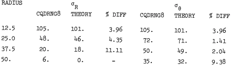
[image:46.568.50.564.27.742.2]

RADIUS ct

R

ae

CQDRNG8 THEORY

%

DIFF CQDRNG8 THEORY

%

DIFF

12.5 105. 101. 3.96 105. 101. 3.96

25.0

48.

46.

4.35

72. 71. i.4i

37-5 20. 18. 11.11 50.

49.

2.04

50.

6.

0. [image:47.568.107.510.183.304.2]

B . THERMAL EXPANSION OF CIRCULAR LISK

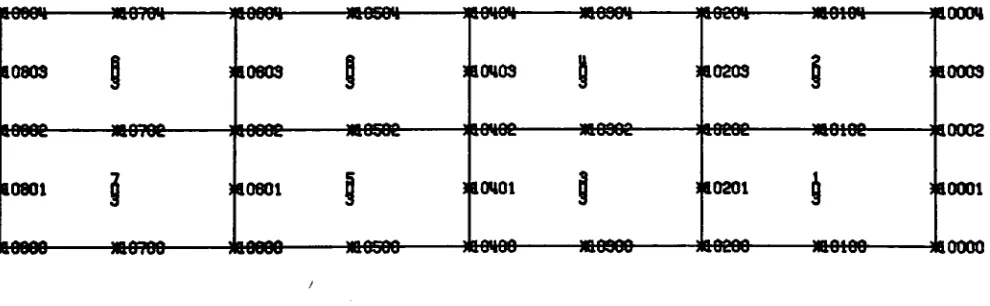
To test the thermoelastic

loading

_capability, a circular disk

with a center hole was subjected to a uniform temperature change.

The temperature of the _ring was raised

by

100

F

_resulting in a

thermoelastic expansion of the disk. Figure

7

is a plot of the

finite element model. Grids are indicated with _ap * . Grid identi

fication numbers are to the right of the *'s. In the center of each

element is the element identification number. The disk was unconstrained

in the radial direction and was constrained at the outside in the axial

direction. As shown in

Timoshenko,

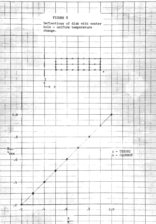
the disk should undergo a stress

free radial and axial growth. Displacement results are shown in Figure

8 and Table

4.

The predicted displacements are _exactly those from

U/18/77

eeeit-)10803

W070M eeeH

310603

xaoscw 3*ete4

sResen-310U03

9ee* moiot

310203

-JjaOOOU

310003

sweee-310801

MOTOe

3weee-310801

IB050S JlOtOfi moooe JlOfiOC woioc -310002

310001

ibesee- _{mo70o ^aoooo 3110500}

310401

3O0H00 HIOOOO

310201

itaoeoo 3P0100 -JHOOOO

FmM8fRJtlEBBflliiSST

[image:49.568.27.522.424.577.2]

;:; FIGURE

8

-7. :

IDeflections of disk with centei

lole

-uniform temperature

* yyy ,. .. .

rr

"

rr -IZLZZZZl-, .

1 rrjrr:

... t.

-T

fl

,

i

s..1::-] J

.. . -1 rrrrrr : ---... i !:-: -

-i -

-" i. ; 1" > ; * < > J > s

' I.i .

-

-::::::

r _Jrrrr

:-::\z:s . .

-:::::_::

... <1 5 1

)

s .i C ._{; s} < 5 .> i

t

i .

.

EErr _{yf.\ ;}

1 rrr ffy7\ .. . z rrrr -:rrr|rr "' '---'- tr-1 -sz::: /

l

J

-77

: '"77-27: ~y

.^ i

:.::

,

i .:::::r : ... .. ... ...

j _r:. ..

fyy-7 zzzJxs.s -..22.

..

rrTrr:-

---:

zzzzzzsr. : :

j 1 ,.___ ! 1 :_: :..

1

j . ; :_4 1 "1" f\ _-.--rr

1 - -

-1

r

_L.U

rrrr i _J

: 1 rrrrrr rrr fyfy :-t=r~ | 1

zszzz.zzzz rr j -yy-yy

:rr|rrT \ ' ! .

!

.y J-₂ " p -ylfs. ti : ---. 0 r /

,. > ..

, ___!____ t

I

A -yj ...

rrrrrrrr

2.2 u

ax ' / \ x

- THEORY

"io - coriRNr.fi

-^

: * rr /

j

-|

-J---\ D &

i _: :.rrrrr

' 1

-

-/

/

i

<

i

---_ 1

1 ' 1 1

\

a / A 1 . . --Z1

f:.:

""]

f / rrrr

2:

.:.-.4 : jay

_

1

j 1 rrrrrr

zz:.::-:. r; -./ 1 ::1r3-~ _. ] I " B

y

P 1 rrr : -- - -i -'--" '-

i

rrrrr

.. .... . .2

4

-;'

I-j

-y

--sz. -.2 -f r:r rrr 7f2l:yf --.

rrrrrrrrrrr: fZffj,yf: :

'-'.._ R t

t ._ ...:.-..-. . -i i -. _R -.:s z-.:r

-Z2f7\2~.~_ \ ~. -::.-:;:.

[image:50.568.41.542.26.745.2]

TABLE

4

-Thermal deflections in disk

RADIUS DEFLECTIONS

CQDRNG8 THEORY

%

DIFFERENCE

10.0 .0010 .0010 0.0

15.0 .0015 .0015 0.0

20.0 .0020 .0020 0.0

25.0 .0025 .0025 0.0

30.0 .0030 .0030 0.0

35.0 .0035 .0035 0.0

40.0

.0040 .0040 0.0

45.0

.0045 .0045 0.0 [image:51.568.123.380.184.339.2]

C THERMAL EXPANSION OF HOLLOW SPHERE

A symmetric section of a hollow sphere was modeled as shown in

the plot of _{Figure 9.} This sphere was subjected to two different

temperature distributions. Symmetric

boundary

conditions were applied

to the cuts of symmetry. Theoretical results from Timoshenko are given.

In the first _case, the sphere is at a uniform temperature which

is 100 F above its reference temperature. The sphere expands _radially

due to the new temperature distribution. As shown in Figure 10 and

Table

5

the CQDRNG8 displacements are _exactly those expected

(0.0

%

error). Since the sphere is _{unconstrained,} all stresses are zero.

The second case considered a linear variation of temperature

through the thickness. This temperature distribution caused internal

bending

stresses. Theoretical

bending

stresses at the surface for a

100aF temperature difference are 2080 psi. The CQDRNG8 predicted

stresses of 1950 psi at the OD and 2250 at the ID. These predicted

FIGURE

9

Plot of hollow sphere model

2/18/77

0104

[image:53.568.34.530.242.745.2]

rrLrr

: ! r.

...:.

t . ._

ir.

1

.-!.:

-. .:.:.::. rrr: L_.. 1 '^1

--i-

-.... .:::y rrrr rrr l.N. -; - -: r.r " I <>

- - ra.

--.:

I

V

r--j -..

. . _B.

-3) ; -y1 ( i -22227 rrrr

- -

X

\-'.-.':

:r:r rr

te

- - j

--- rrr rrrr

R . . '. .;::.: :

rrr

r rrjrr_

50 in in '* . _..j. y . -"

^40

-: rrr - - -- - _._...

rrfrrrj

: _._... -- - -1 :rrr ] .00

""--''- i

. ---

-7--- -- -rrrr __.

1

__, /- -- -- -i ]

-rrrr._rrrrrr

/

rrrr

r

"T

.OR i

/ ' j

\I

X - THEOF Y

..rrrrr 1 i

y

i / i ---

-/

!

o -CQDRN

G8.

i ur

Ur

_rmax

y

i

;

Lon

1 i j i - r-.PF,

2.2. .

-- ..

.fio

I-'- .. . - -

-rr.:. r.

< "

30 .

35

oo

95

1 (W - ___:_-..

-

j-*Wx

[image:54.568.41.547.26.750.2]

---TABLE

5

-Thermal

expansion of hollow sphere

RADIUS RALIAL DEFLECTION

CQDRNG8 THEORY

%

DIFFERENCE

40.0

.00400 .00400 0.0

42.5

.00425 .00425 0.0

45.0

.00450 .00450 0.0

47.5

.00475 .00475 0.0 [image:55.568.109.368.172.267.2]

D. HEAT FLOW IN A CIRCULAR DISK

To demonstrate the convergence of the C0.DRNG8 element, the prob

lem of heat flow in a circular disk was solved. The disk has a small

centerhole constrained to 0.0aF. The outer diameter of the disk is

constrained to 100. 0*F. This problem was solved _using the three dif

ferent discretizations shown in Figure ll* The models contained

8,

2,

and 1 CQDRNG8 elements respectively. The problem was also solved

using three similar gridworks of CTRIARG elements. These models are

shown in Figure 12. The CTRIARG is a three noded triangular _ring

element which _currently exists in NASTRAN. Each CQDRNG8 element has

been filled with eight CTRIARG elements and an additional degree of

freedom has been added at the center. The CTRIARG element has a

linear temperature variation as compared to the quadratic variation

of the CQDRNG8 element.

The results of this study are shown in Figure

13

and Table 6..

22

Theoretical results are from Carslaw. For the coarsest model, the

1 CQDRNG8 element with 2 unconstrained degrees of freedom gives the

same results as 8 CTRIARG elements

having 3

dof. The temperatures

are in error

by

_10.57

%.

The 2 element CQDRNG8 model with

7

uncon

strained dof predicts temperatures which are in error

by

I.58 to

12.16

%.

The CTRIARG model with 16 elements and

9

unconstrained

dof predicts temperatures greater in error. The error in the CTRIARG

model ranges from

2.23

to 13.70

%

In the finest models, the CQDRNG8

with 8 elements and

27

unconstrained dof has a maximum error of 9.96

%

The CTRIARG model with 64 elements and

55

unconstrained dof had a

In all _cases, the CQDRNG8 models had one-eighth the number of

elements and at least one-fourth fewer degrees of freedom than the

CTRIARG models. For the coarest model, the single CQDRNG8 element

was comparable to the eight CTRIARG elements. For the other models,

a moderate increase in _accuracy was realized. The CQDRNG6 element

does exhibit the convergence characteristic. Each refinement of the

FIGURE 11 a

Circular disk model

1 CQDRNG8 element

2 unconstrained dof

tl/28/77

360002

380001

330000

FIGURE 11 b

Circular disk model

2 CQDRNG8 elements

7

unconstrained dof

1/28/77

tf₀₀₀₂

ikiooi

^eoooo

[image:59.568.51.539.442.552.2]

[image:60.568.69.549.445.556.2]

FIGURE 11 c

Circular disk model

8 CQDRNG8 elements

27

unconstrained dof

U/28/77

3M8M-110803

I

WwC-3W070H

*wee<*-310803

3B0SOH 3I0H0H

310U03

3HW--jwse**-

3eeH-310203

310B02

W010H

3B010C

-31000U

310003

-310002

310001

-310000

M070C

310801

318888- _K10700

3ieeee- _{mosog wosoa}

310801

itaoeoo

I

3110500

3I0H01

3WWfr- _3B0800

310201

ifaoeoo 3P0100

aiSWfcWWIffl

fl L. .T.E9T

FIGURE 12 a

Circular disk model

8 CTRIARG elements

3

unconstrained dof

tl/28/77

480002

0000

[image:61.568.64.554.430.537.2]

U/28/77

FIGURE 12 b

Circular disk model

16 CTRIARG elements

9

unconstrained dof

3C0002

iteoooo

[image:62.568.64.553.447.556.2]

[image:63.568.49.544.442.550.2]

FIGURE 12 c

Circular

disk model

64

CTRIARG elements

35

unconstrained dof

1/27/77

13

Circular disk temperatures Convergence test

L33I33L

:r}rr

^y

--.%-rfcrzr:

jy

yy.

M

THEORY

JJ: o ₆₄ CTRIARG

(35

dof)

3L3n 16 CTRIARG

(

9

dof)

-- a 8 CTRIARG

(

3

dof)

X 8 CC4DRNG8

(27

dof)

y

+ _{2 CQDRNG8}

(

7

dof)

O 1 C<-DRNG8

(

2

dof)

3E-iifi

-313333

E33333

^fe

703

,333

3t333

333311

33F.3

R!

iax

[image:64.568.40.546.35.744.2]

TABLE

6

- Circular

disk temperatures - _convergence test

RADIUS TEMPERATURES

THEORY CTRIARG RESULTS

35

dof

%

Diff

9

dof

%

Diff

3

dof

%

Diff

1.000 0.0 0.0 0.0 0.0 0.0 0.0 0.0

7.125

50.1942

44.00

12.35

13.250

66.0527

61.51

6.86

57.OO 13.70

19.575

75.7660 72.46

4.36

25.500 82.7878

80.41

2.86

77.93

5.86

74.03

10.

57

31.625

88.2906

86.67

I.83

57.750 92.8161 91.82

1.07

90.75

2.13

43.875

96.6246

96.19

.45

50.000 100.000 100.00 0.0 100.00 0.0 100.00 0.0

RADIUS TEMPERATURES

THEORY CQDRNG8 RESULTS

27

dof

%

Diff

7

dof

%

Diff 2 dof

%

Diff

1.000 0.0 0.0 0.0 0.0 0.0 0.0 0.0

7.125

50.1942

45.19

9.96

13.250

66.0527

63.22

4.28

58.02 12.16

19.375

75-7660 73.71 2.71

25.5OO 82.7878 81.34 1.74 79-36

4.13

74.02

10.57

31.625

88.2906 87.30 1.12

37.750 92.8161 92.21 .65

91.35

1.58

43.875

96.6246 96.38 _.25 [image:65.568.75.461.181.572.2]

E. HEAT FLOW IN AN AXIAL ROD

Temperatures were determined in an axial rod with constrained

end temperatures. The theoretical solution from Carslaw predicts

a linear temperature variation through the rod. The model and

results are shown in Figure 14. The CQDRNG8 model predicts the

[image:67.568.37.543.30.745.2]

F- HEAT FLOW IN A HOLLOW SPHERE

The final thermal test case is that of a hollow sphere. The

sphere is analyzed for two sets of

boundary

conditions. The first

case is that of constrained temperatures at both the inner and outer

diameters. The theoretical solution is presented in Carslaw. The

finite element model is the same as that shown in Figure 9 Figure

15

and Table

7

show both the

theory

and CQDRNG8 results. For this

case, the CQDRNG8 results are exact

(0.0

%

error).

For the second case, the inner diameter temperatures are con

strained and the outer diameter is subjected to convection. To

represent the convection

boundary

_condition, special NASTRAN heat

transfer

boundary

condition elements

(CHBDY)

must be used in con

junction with the CQDRNG8 elements. The

theory

for this case is

also found in Carslaw. Figure 16 and Table 8 show the comparison

.rrr:rrr K.

"rtl1 T

-:::f2:i-i riil

rr.r

rr:

: 11

rr:

r:n_rnl rr rr .:.::

-,.. 33c:

,:::j

iT 1 711 _. J

_+^-.rrr . : rr

-rr: rrrr_..<t..

<S

y

-._ sr:11:1sz. -222-

'::'::-777r~Ki

-; r:.rrrrIr2- rrr:

'

,

--- -

-i>,._

*. -1*. .:/. .sr.

.7777 jlr..rr r. lil. zr. r :::r sly .: Tr r rrr -'----:-- - -r -r-r: -"-r -s-: -r.r -1?-y.~ 77V i-i 7 .. . f

rLrr ;;: ._..

*

L

-*T- ..:::rrr rrr: rrr

rr

A

:y -72. r

-

;-'

. : r -'2

:r:

-t

--- s- --.

K sz: ---

-\zr. \ -

V--V

.rr rr: .:..:

rr: 1'

;

rrr rrlr -:r:r rr. rr: rrr: rrr r : :

R: :l:rlrrr 11:1' --v

-x

.... r n -.: rrr ..:::rr: ":z .rrr.rrrrrrr rrrrrrr T - -i i ....

rr rr. rr.

r :r _rrr| _ -^ ', t:

rrr_"rr rrr

---rrrr

rrr1777717 rr: 1 i2z 27z'zKl Kl

..-- .

;:3:- r

-7: 7 22.7Ki

\'- -: -... -- -777-

-H-r-7-7- rrrr rrrr rrr:

rrrirrr r-rr

.. ___.- - '

~^-k

"" i ""rt" "

rrrrr rrrr rl: rrr

rr rrrrrrrrrr

''-7-.::

:-_-:Kl2727rrr

x.u.

-7-rrr: rr:

1 77

"

rrrKrlri11 Kl-11: -r-rrIKrrrr. rrr rrrr r~rr_,

--Kl

rrr

-Lrrr

''-'--:::-rrr: -rrrr

I :

-rrrrrrrrr[-:r -rrr :'~-7

--___

rrrr rrrr

,---rrl

K

f""r -1. ss r

t-: '& r : }

-.rrrrrrr.-777

-; - i

rrrr:rrrrr

r i

y

r" "! :rrr rrr - ---=7

:--r'lrKlrrr rrrr

-: -:. -: r

72/

szz: " ^K 7.

^y

-rrr rrr

rrr~r .__r

:_

rrrr rrrr:rrrr: rrrr r-.-₁₇

:r-722

.r ;

3:;- rr -rrr

-Trr ----

---

y7-"

^r

-maxQ7-.cH

--^ ^r-rr -"j7:

f

^ II :rr --:- :s:-rr: -.:--:.-.sr

1 - "

L7::

rrrr-rr

,

-7 ... - -

-- i ... ,. -: f " " .. [

-sz: /-

----rrrr rrr r :;

;-

-rrr --./ -I ..:: : r:

x :THI

OR^} -r ---(rrrrr rrrr rr: rr: j'

I

lri

rrrr7227 K

::::: 6 COI RC

-K

rrt \

'

;, r

K--'- ':'--:

3-3 rlL

lr: zz . :h

- ;----__r; j rrr.

t

rrr

7-rr-/

---722: sr.

-

:..:!:--rrr

'

. . .

rrr

rrrrrrrr) -:r _7-2

-.

i: --

-'

i

rr ^__-._;rrr rrrr

K rrr -sz7'7-Z rr : r

--- -7- ""

7 177 7

- -- ₁

_, i

-rcr

L

-/

--- -rr ss: rrr:

- 1

K- -

-i- --

-j ;i

"I rr -.szrr rr rrrr r: rr

7 7"! 7 17Fi":

r _r rrr

;

--; s

/--'-'-'-'- ":---T rr rrr

i

-i

.: rL:. r

r rr ' j"

1 ^

Vi

, l -7

y

*-i'.r l 1 r

[image:69.568.33.540.30.685.2]

TABLE

7

-Temperatures in hollow sphere

Enforced temperatures at surfaces

RADIUS _TEMPERATURES

CQDRNG8 THEORY

%

DIFFERENCE

40.0

100.00 100.00 0.0

42.5

129.41 129

4l

0.0

45.0

155.56 155-56 0.0

47-5

178.95 178.95 0.0 [image:70.568.116.379.177.303.2]

[image:71.568.43.550.30.762.2]

TABLE 8

-Temperatures in hollow sphere

Enforced temperature at ID Convection at OD

RADIUS TEMPERATURES

CQDRNG8 THEORY

%

DIFFERENCE

40.0

42.5

45.0

47-5

50.0

100.00

127-97

152.84

177-05

199-04

100.00 128.28 153.42

175.91

196.15

.0

.24

.38

.65

[image:72.568.140.396.125.325.2]

G. _{THERMOELASTIC STRESSES IN A HOLLOW CYLINDER}

Schlottner presented a finite difference solution for transient

thermal stresses in a hollow cylinder. The _cylinder, at a uniform

initial temperature and with convection at the outer

diameter,

was

subjected to an increase in the ambient temperature. The _resulting

transient temperature distributions create internal stresses. Since

the CQDRNG8 element does not include a transient heat transfer _cap

ability, the heat transfer portion of the problem could not be solved.

However thermal stresses could be determined at particular time steps

if a reasonable estimate of the temperature distribution could be

made. Schlottner's solution gives the temperatures at the ID and OD

of the hollow cylinder at various times. For a _{first approximation,}

the temperature distribution through the cylinder was assumed to be

linear. The finite element model is shown in Figure 17. As shown

in Table 9, . the stresses for the two time steps listed are approx

imately

10.0 to 25*0

%

lower than those predicted

by

Schlottner. A

second approximation of the temperature distribution was arrived at

by

solving the steady state heat problem _using

boundary

conditions

A-U

from Schlottner'

s solution. At the 26 time step of Schlottner

's

solution, the OD temperature was close to a _steady state condition

but the ID temperature was not. For the steady state problem _solved,

the ID temperature was constrained to the value predicted

by

_Schlottner

4/12/77

xioaco "Qoaoi xicaoa xaoaos yioao'j xioaos xioaos xioao7 3*10209

3S01CC 1D3 310102 2D3 310104 303 sa0106 403 SSOiOS

XiOOOO X10001 X10002 X100Q3 X10004 X10005 XXOCOO XG0007 3I90CG9

[image:74.568.120.484.430.554.2]

TABLE

9

- Stresses in hollow

cylinder

TIME SCHLOTTNER LINEAR TEMP

%

SS TEMP

%

STEP STRESS STRESS DIFF STRESS DIFF

ID OD ID OD ID OD ID OD ID OD

15 16000 19000 12000 14000 25.0 26.3

shown in Table

9,

this resulted in -poorer correlation at the ID

but much poorer correlation at the OD.

This comparison is

by

no means a rigorous test of the CQDRNG8

element's capabilities and is _{included only to} provide a comparison

to another numerical method. To determine the correct thermoelastic

stresses, the correct temperature distribution must be known. Con

sidering the approximate nature of the temperature assumption, the

VII. SUMMARY

The development and application of an axisymmetric finite element

for the NASTRAN computer program has been presented. The element is

an eight noded _{isoparametric} quadrilateral _ring with an assumed

quadratic displacement and temperature function. The element has

been named CQDRNG8. Element capabilities include elastic stiffness

for homogeneous isotropic _materials, thermoelastic

loading,

heat

conduction for homogeneous isotropic materials, deformed and

unde-formed plotting, and stress recovery. Stress invariants calcu