White Rose Research Online URL for this paper:
http://eprints.whiterose.ac.uk/125352/
Version: Accepted Version
Proceedings Paper:
Heywood, P., Richmond, P. and Maddock, S. orcid.org/0000-0003-3179-0263 (2015) Road
Network Simulation Using FLAME GPU. In: Euro-Par 2015: Parallel Processing
Workshops. Euro-Par 2015 International Workshops, 24-25 Aug 2015, Vienna, Austria.
Lecture Notes in Computer Science, 9523 . Springer, Cham , pp. 430-441. ISBN
978-3-319-27307-5
https://doi.org/10.1007/978-3-319-27308-2_35
[email protected] https://eprints.whiterose.ac.uk/
Reuse
Unless indicated otherwise, fulltext items are protected by copyright with all rights reserved. The copyright exception in section 29 of the Copyright, Designs and Patents Act 1988 allows the making of a single copy solely for the purpose of non-commercial research or private study within the limits of fair dealing. The publisher or other rights-holder may allow further reproduction and re-use of this version - refer to the White Rose Research Online record for this item. Where records identify the publisher as the copyright holder, users can verify any specific terms of use on the publisher’s website.
Takedown
If you consider content in White Rose Research Online to be in breach of UK law, please notify us by
Peter Heywood, Paul Richmond, and Steve Maddock
Department of Computer Science, The University of Sheffield, UK
{ptheywood1,p.richmond,s.maddock}@sheffield.ac.uk
Abstract. Demand for high performance road network simulation is in-creasing due to the need for improved traffic management to cope with the globally increasing number of road vehicles and the poor capacity utilisation of existing infrastructure. This paper demonstrates FLAME GPU as a suitable Agent Based Simulation environment for road network simulations, capable of coping with the increasing demands on road net-work simulation. Gipps’ car following model is implemented and used to demonstrate the performance of simulation as the problem size is scaled. The performance of message communication techniques has been evalu-ated to give insight into the impact of runtime generevalu-ated data structures to improve agent communication performance. A custom visualisation is demonstrated for FLAME GPU simulations and the techniques used are described.
Keywords: Parallel Agent Based Simulation, FLAME GPU, Transport Network, Performance Scaling, Visualisation
1
Introduction
With the increasing number of vehicles on road networks around the world and poor utilisation of existing road infrastructure capacity, there is a need for im-proved systems for planning and trialling proposed changes to traffic manage-ment system [16, 26]. To avoid making costly or risky changes in the real world, computer modelling and simulation can be applied to evaluate proposed solu-tions. Transport simulation models can typically be classified into one of three categories: macroscopic, mesoscopic and microscopic. Macroscopic simulations (top-down) treat traffic as a liquid, modelling the overall system level behaviour. Mesoscopic simulations (middle-out) model platoons (groups of vehicles), using aggregate functions to calculate travel times and speeds [6]. Microscopic simula-tions (bottom-up) model the individual vehicles in the system and the interaction between them [23], and can be considered synonymous with Agent Based Simu-lations (ABS) [5]. In ABS behaviours are modelled at the individual level with agents interacting with both the local environment and other agents. Higher sys-tem level behaviours can emerge from the lower level behaviours and interactions modelled by the system.
scale and more-complex microscopic simulations are computationally expensive [3] when being processed in serial, but have been shown as suitable for accel-eration through parallel methods [15, 20]. Each agent in the system follows the same model, performing the same operations, as other agents of the same type, making aspects of microsimulation SIMD (Same Instruction Many Data) in na-ture and therefore an ideal task for General Purpose computing on Graphics Processing Units (GPGPU), which is well suited to SIMD problems. GPGPU computing has been shown to be effective for microsimulation of transport sys-tems [24, 27] and the associated tasks [7], showing that it can be used to provide computational speed-up or allow increased complexity for a similar execution time, while using low cost hardware.
This paper demonstrates the performance implications of applying the Graph-ics Processing Unit (GPU) to microsimulation of transport networks. It makes a unique contribution by evaluating performance scalability through the imple-mentation of an artificial road network in which the size of the road network and the density of traffic within it can be effectively benchmarked. The Gipps car following model has been implemented using theFlexible Large-scale Agent Modelling Environment for Graphics Processing Unit (FLAME GPU) frame-work and the message communication techniques have been evaluated to give insight into the impact of runtime generated data structures to improve agent communication performance. A custom visualisation using GPU instancing has been developed which enables interactive simulation observation. The improved simulation performance described by this work is important in demonstrating simulations which are able to handle the increasing scale and complexity which are required to accurately model transport networks of increasing size. A cou-pled visualisation has the additional benefit of ensuring that traffic simulation is accessible to stakeholders involved in traffic management and infrastructure changes who are often non-modelling specialists [16].
2
Related Work
Transport microsimulation models have been used to analyse and study a broad range of driver behaviours, infrastructure layouts and the effects of traffic [4, 9, 19, 12], showing that there are real world uses for microsimulation of trans-port systems for both analysis and planning without the need for costly and potentially dangerous real world experimentation.
For any study of transport systems at the microscopic level, driver behaviours such as car following [10, 25], lane changing [11], interaction with road signals or traffic calming measures [13], amongst others, need to be modelled to achieve a valid, fully functional system which can be used to study other aspects of transport network behaviours.
lane on sections of road with multiple lanes, vehicle drivers wish to drive at their desired speed without colliding with the vehicle ahead [11].
The car following theory is that a driver reacts to the behaviour of the car(s) in front. Early models were mainly concerned with the trailing car’s acceleration being proportional to the relative speeds of each car at an earlier time, or a ‘history’ of relative speeds [14]. Later models took into account the reaction time of the vehicle driver [10], as there is a delay between an individual receiving stimuli and performing the correct action.
The performance limits of both the driver and vehicle also affect car following behaviour, as safety concious drivers will ensure there is a gap large enough in which to stop between them and the vehicle in front (limited by an acceptable level of braking). Vehicles also have limits of acceleration performance, and so a trailing car will accelerate with no more than the vehicle’s maximum acceleration until it nears the desired speed (or the speed of the vehicle in front) at which point the rate of acceleration will decrease to zero [10]. Models which are based on the principal of following at a safe distance such as Gipps’ model are known assafety distance models.
Other models and categories of car following models have been developed, such as theIntelligent Driver Model proposed by Treiber et al [25]. At it’s core this model bases the acceleration of the trailing vehicle on the ratio between the “desired minimum gap” and the actual gap to the vehicle in front, with special cases for scenarios such as when traffic is in equilibrium where drivers will keep a gap to the vehicle in front which is dependant on velocity.Psycho-physical car following models are an alternate category in which models adjust the reactions of the driver based on the state of the vehicle [22].
3
Model
In order to demonstrate the scalable performance of Agent Based Simulations using an accelerator such as the GPU, Gipps’ Car Following Model [10] was selected for implementation as it is one of the most extensively used car following models [8].
The model aims to “mimic the behaviour of real traffic”, have “parameters which correspond to obvious characteristics of drivers and vehicles” to avoid elaborate calibration procedures and “should be well behaved when the interval between successive recalculations of speed and position is the same as the reac-tion time”[10]. The model combines limits on the performance of the driver and vehicle with the assumption that a following driver will drive in such a manner that they can safely stop if the vehicle ahead stops suddenly.
The model states that the vehiclenshould not exceed its driver’s target speed and the vehicle’s free acceleration should increase with speed then decrease as the desired speed is approached [10]. The inequality in Equation 1 combines these two constraints:
vn(t+τ)<=vn(t) + 2.5anτ(1−vn(t)/Vn)(0.025 +vn(t)/Vn)
1
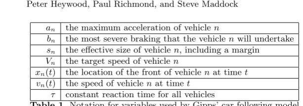
an the maximum acceleration of vehiclen
bn the most severe braking that the vehiclenwill undertake
sn the effective size of vehiclen, including a margin
Vn the target speed of vehiclen
xn(t) the location of the front of vehiclenat timet
vn(t) the speed of vehiclenat timet
[image:5.595.141.448.94.202.2]τ constant reaction time for all vehicles
Table 1.Notation for variables used by Gipps’ car following model
The terms of Equation 1 are explained in Table 1. The limitation of braking safely can be represented by the inequality shown in Equation 2. This takes into consideration the following driver’s reaction time, and a margin of error on the driver’s behalfθ=τ /2 to avoid maximum braking and an estimate of the leading driver’s most severe braking ˆbwhich cannot be estimated by direct observation [10].
vn(t+τ)<=bnτ+
q
bn
2
τ2
−bn(2[xn−1(t)−sn−1−xn(t)]−vn(t)τ−vn−1(t)2/ˆb)
(2) Assuming that if the driver travels as fast as safely possible considering ve-hicle limitations, the new speed can be given by Equation 3.
vn(t+τ) = min
vn(t) + 2.5anτ(1−vn(t)/Vn)(0.025 +vn(t)/Vn)
1 2,
bnτ+
q
bn
2
τ2
−bn[2[xn−1(t)−sn−1−xn(t)]−vn(t)τ−vn−1(t)2/ˆb]
(3)
The main restriction of Gipps’ car following model is that the time-step of the simulation needs to be set to the driver reaction time τ. The model also relies on assumptions that drivers drive in a safe manner (which is often not the case) and that they are capable of estimating observable characteristics of the leading vehicle with some degree of accuracy.
4
Implementation
This section consists of four parts: the artificial road network, an overview of FLAME GPU, how Gipps’ car following model is implemented using FLAME GPU & the visualisation.
4.1 Scalable Artificial Road Network
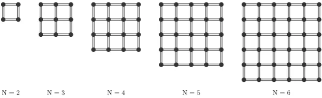
with real world limitations such as terrain or the location of existing roads, buildings and other spatial constraints. An artificial road network is preferable for performing controlled studies as the properties of the road network are con-sistent at different scales. The artificial road network is a uniform grid network, generated based on the target grid sizeN whereN >= 2, as shown in Figure 1. The grid containsN rows andN columns of junctions, with two sections of road between each adjacent node, hence the road network containsN2
junctions and 4N(N−1) one-way sections of road.
[image:6.595.143.472.239.339.2]N = 2 N = 3 N = 4 N = 5 N = 6
Fig. 1.Examples of the artificial road network with varying values ofN. Circles rep-resent junctions and lines reprep-resent sections of road
4.2 FLAME GPU
FLAME GPU [21] is a “template based simulation environment” for agent based simulation on Graphics Processing Unit (GPU) architecture. Agents are repre-sented as X-Machines which can communicate via globally accessible message lists. Messages are crucial for interaction between agents and they can be parti-tioned to “ensure the most optimal cycling of messages”[21].
There are currently three defined message partition schemes in FLAME GPU: non-partitioned, discrete 2D space partitioning and 2D/3D spatially partitioned space. Non partitioned messaging involves no filtering to reduce the number of messages each agent must iterate; it is merely a brute force approach. Discrete partitioned messages can be used only when sending from non mobile discrete agents, and is therefore best suited to discrete systems using Cellular Automata (CA) based approaches.Spatially partitioned messages originate from agents in continuous space (such as a 2D or 3D environment). The partitioning scheme requires a radius and environment bounds. The radius dictates the range to which the message iteration will extend to from its originating point, while the bounds are used to limit the area of partitioning.
Of these partitioning schemes both non partitioned messaging and spatially partitioned messaging are of interest with potential performance implications. Non partitioned messaging is computationally expensive (O(n2
to dynamic construction of data structures compared to partitioned messaging schemes. Simulations using partitioned messaging generally lead to less expen-sive message iteration loops but an increased overhead cost as long as the par-titioning system is set-up appropriately. Both non partitioned messaging and spatially partitioned messaging will be evaluated and the performance difference compared.
4.3 Implementing Gipps’ Car Following Model using FLAME GPU
Each vehicle in the system is represented by an agent. The initial values of each agent are generated by a Python script and stored in a FLAME GPU XML file for simulation state data to be parsed at runtime and copied into device memory. The road network is stored in CUDA constant memory (via FLAME GPU’s Simulation Constants) as it will not change over the course of the simulation and each agent in the simulation interacts with the same road network. This does however impose a limit on the number of nodes and roads possible within the system, due to the current limit of 64kB of constant memory being available. An alternative would be to store the road network in the CUDA Read-Only Data Cache [17] but this would restrict the GPU architectures which could be used to CUDA Compute Capability 3.0 (Kepler) and greater.
For each step in the simulation, each agent first outputs it’s observable prop-erties (location, velocity, etc.) as a message using the selected message partition-ing scheme. Each vehicle then iterates through the list of relevant messages based on the partitioning scheme to find the message from the lead vehicle. Gipps’ car following model (Section 3) is applied to the current vehicle, using the Forward Euler Method to calculate the vehicle’s new location and velocity. Higher-order integration methods could be considered, with further related study on accuracy and performance trade-offs. Agents which have reached the end of their current segment of road randomly select a new segment from the roads connected at their current junction.
4.4 Visualisation and Graphics Techniques
5
Experimental Results
Two sets of benchmarking experiments are carried out to evaluate 1) the perfor-mance of the simulation as the number of agents within the system is increased, and 2) the overall scale of simulation while maintaining a fixed vehicle to road ratio. The two message partitioning schemes are compared and the performance difference highlighted for each set of experiments. Agent populations are gener-ated using the model parameters defined in Table 2 and randomly distributed throughout the road network. The simulation has been implemented in FLAME GPU 1.4 for CUDA 7.0. Results are obtained from an Intel Core i7 4770K ma-chine using an NVIDIA TESLA K20c GPU with CUDA 7.0.
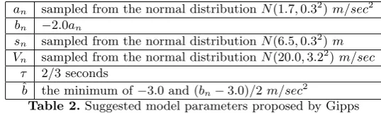
an sampled from the normal distributionN(1.7,0.32)m/sec2
bn −2.0an
sn sampled from the normal distributionN(6.5,0.32)m
Vn sampled from the normal distributionN(20.0,3.22)m/sec
τ 2/3 seconds
ˆ
[image:8.595.171.440.268.348.2]b the minimum of−3.0 and (bn−3.0)/2m/sec2
Table 2.Suggested model parameters proposed by Gipps
5.1 Vehicle scaling for static road network
The first experiment illustrates the performance scaling of the agent based sim-ulation with respect to the number of agents in the system. A fixed grid network of size N = 16 and road length of 10000m is used and the number of agents varies from 28
up to 218
, using both message partitioning techniques.
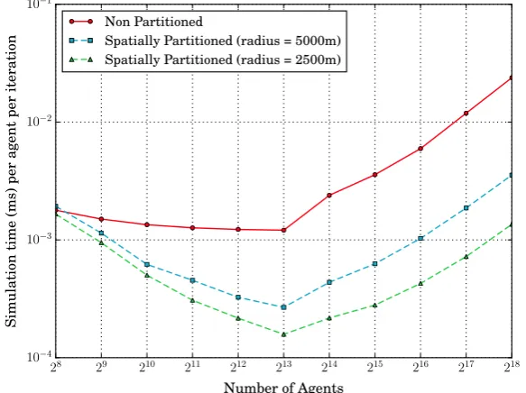
Figure 2 shows the performance against the number of agents, where perfor-mance has been measured by averaging the simulation time over 100 iterations. At very small numbers of agents, non partitioned messaging demonstrated sim-ilar performance to partitioned messaging, but with greater numbers of agents the gap in performance increases dramatically with each increase in agent popu-lation size. Spatially partitioned messaging shows a similar level of scaling with each radius, but the lower radius consistently shows higher levels of performance. Figure 3 shows the average agent iteration performance (calculated as av-erage iteration time / population size). With small agent counts (<= 213
), as the population size increases the simulation performance increases as hardware utilisation increases. Larger populations (>213
amount of messages, but still less than would be received using the brute force approach.
The larger population sizes show a decrease in per agent performance for each increase in agent population, with a significant decrease in performance for non partitioned messaging when compared to spatially partitioned messaging.
5.2 Scaling of vehicle and road network
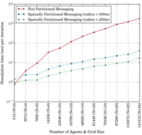
The second experiment illustrates the performance scaling of the agent based simulation with respect to the problem size as a whole - the number of agents and size of grid generated have been scaled in unison, maintaining a constant vehicle count per section of road (64 vehicles per 1000m of road) from N = 2 & 512 agents to N = 24 & 141312 agents, with a road length of 1000m. The vehicle to road ratio is kept constant to illustrate the performance difference from increasing the size of the problem as a whole, rather than just increasing the density of vehicles. Both message partitioning techniques are used and the performance difference highlighted, including using different spatial partitioning radii (250mand 500m).
Figure 4 shows the performance against the scale of simulation, where perfor-mance has been measured by averaging the simulation time over 100 iterations. This shows that as the overall size of simulation is scaled up the simulation time also increases. Non partitioned messaging shows greater performance at very small simulation sizes compared to partitioned communication. This is due to the additional computational overhead of spatial partitioning. Larger problem sizes show the benefits of using a partitioned messaging scheme to reduce the number of messages each agent must iterate through, as the performance impact of a greater problem size is significantly less for larger problem sizes. For a grid size of N = 24 average iteration time was approximately 44.4 & 103.4 times quicker using spatially partitioned communication with radii of 500m & 250m
respectively than non partitioned messaging.
This experiment was initialised with uniform vehicle distribution. Whilst uneven distributions then occur as the simulation progresses, future work needs to consider this aspect and any associated performance implications in more detail.
5.3 Visualisation
28 29 210 211 212 213 214 215 216 217 218
Number of Agents
10−1
100 101 102 103 104
S
im
u
la
ti
on
ti
m
e
(m
s)
p
er
it
er
a
ti
on
Non Partitioned Messaging
[image:10.595.165.452.127.353.2]Spatially Partitioned (radius = 5000m) Spatially Partitioned (radius = 2500m)
Fig. 2. Average iteration execution time for fixed grid of sizeN = 16 against agent population size, averaged over 100 iterations
28 29 210 211 212 213 214 215 216 217 218
Number of Agents
10−4
10−3
10−2
10−1
S
im
u
la
ti
on
ti
m
e
(m
s)
p
er
a
g
en
t
p
er
it
er
a
ti
on
Non Partitioned
Spatially Partitioned (radius = 5000m) Spatially Partitioned (radius = 2500m)
[image:10.595.162.454.396.614.2]5 1 2 (N = 2 ) 3 0 7 2 (N = 4 ) 7 6 8 0 (N = 6 ) 1 4 3 3 6 (N = 8 ) 2 3 0 4 0 (N = 1 0 ) 3 3 7 9 2 (N = 1 2 ) 4 6 5 9 2 (N = 1 4 ) 6 1 4 4 0 (N = 1 6 ) 7 8 3 3 6 (N = 1 8 ) 9 7 2 8 0 (N = 2 0 ) 1 1 8 2 7 2 (N = 2 2 ) 1 4 1 3 1 2 (N = 2 4 )
Number of Agents & Grid Size
10−1
100 101 102 103 104 S im u la ti on ti m e (m s) p er it er a ti on
Non Partitioned Messaging
[image:11.595.164.452.125.397.2]Spatially Partitioned Messaging (radius = 500m) Spatially Partitioned Messaging (radius = 250m)
Fig. 4.Average iteration execution time for increasing Grid SizeNwith a fixed vehicle
density of 64 agents per 1000m, averaged over 100 iterations
(a) Nearby (b) Overview
[image:11.595.135.478.457.637.2]6
Conclusions
Two experiments have been carried out, demonstrating that GPUs are suitable for Agent Based Simulation of road networks and are capable of scaling to han-dle the increasing demands of road network simulations, and the performance difference between message partitioning schemes is highlighted.
Both experiments show that FLAME GPU can successfully be used for agent based simulations of road networks and can process large amounts of agents in a reasonable time frame. The experiments also highlight the performance dif-ference between the two message partitioning techniques. Non partitioned mes-saging only outperforms spatially partitioned mesmes-saging when the number of agents in the system is low enough that the additional overhead of the parti-tioning scheme outweighs the performance improvements and so for agent based simulations where a generally large populations of agents are used spatially par-titioned messaging is more suitable, but the choice of spatial partitioning param-eters need to be selected carefully. Smaller partitioning radii generally increases the performance but the radius needs to be relevant to the target simulation so that messages from relevant agents still reach each other.
Future work developing alternate message partitioning techniques specific to networked systems should allow further increase in performance compared to spatially partitioned messaging. On a road network a driver is only concerned with vehicles on the same section of roads and connected sections of roads at junctions. Developing a messaging scheme which limits the incoming agent mes-sages to the road network structure should reduce the cost of the message itera-tion loop, without too large of a performance overhead. An example visualisaitera-tion has also been described, demonstrating some of the techniques which can be used to create custom visualisations for FLAME GPU based simulations.
References
1. OpenGL SDK glDrawArraysInstanced manpage.https://www.opengl.org/sdk/
docs/man/html/glDrawArraysInstanced.xhtml
2. Simple DirectMedia Layer (libSDL).https://www.libsdl.org/
3. Algers, S., Bernauer, E., Boero, M., Breheret, L., Di Taranto, C., Dougherty, M., Fox, K., Gabard, J.F.: Review of micro-simulation models. Institute for Transport Studies (1997)
4. Bell, M.C., Galatioto, F., Giuffr`e, T., Tesoriere, G.: Novel application of red-light runner proneness theory within traffic microsimulation to an actual signal junction. Accident Analysis & Prevention 46, 26–36 (2012)
5. Bonabeau, E.: Agent-based modeling: Methods and techniques for simulating hu-man systems. Proceedings of the National Academy of Sciences 99(suppl 3), 7280– 7287 (2002)
6. Charypar, D., Axhausen, K.W., Nagel, K.: Event-driven queue-based traffic flow microsimulation. Transportation Research Record: Journal of the Transportation Research Board 2003(1), 35–40 (2007)
8. Ciuffo, B., Punzo, V., Montanino, M.: Thirty years of gipps’ car-following model. Transportation Research Record: Journal of the Transportation Research Board 2315(1), 89–99 (2012)
9. Garc´ıa, A., Torres, A.J., Romero, M.A., Moreno, A.T.: Traffic microsimulation study to evaluate the effect of type and spacing of traffic calming devices on ca-pacity. Procedia-Social and Behavioral Sciences 16, 270–281 (2011)
10. Gipps, P.G.: A behavioural car-following model for computer simulation. Trans-portation Research Part B: Methodological 15(2), 105–111 (1981)
11. Gipps, P.G.: A model for the structure of lane-changing decisions. Transportation Research Part B: Methodological 20(5), 403–414 (1986)
12. Keenan, D.: M 62-m 1 interchange- a combined transyt/vissim micro-simulation assessment. Traffic Engineering+ Control 46(5), 178–187 (2005)
13. Kesting, A., Treiber, M., Helbing, D.: General lane-changing model mobil for car-following models. Transportation Research Record: Journal of the Transportation Research Board 1999(1), 86–94 (2007)
14. Lee, G.: A generalization of linear car-following theory. Operations Research 14(4), 595–606 (1966)
15. Nagel, K., Rickert, M.: Parallel implementation of the transims micro-simulation. Parallel Computing 27(12), 1611–1639 (2001)
16. Neffendorf, H., Fletcher, G., North, R., Worsley, T., Bradley, R.: Modelling for intelligent mobility (Feb 2015)
17. Nvidia, C.: CUDA Kepler Tuning Guide - Read-Only Data Cache.http://docs.
nvidia.com/cuda/kepler-tuning-guide/#read-only-data-cache
18. Nvidia, C.: Cuda c programming guide. http://docs.nvidia.com/cuda/pdf/
CUDA_C_Programming_Guide.pdf(Mar 2015), last accessed 2015-03-30
19. Panis, L.I., Broekx, S., Liu, R.: Modelling instantaneous traffic emission and the influence of traffic speed limits. Science of the total environment 371(1), 270–285 (2006)
20. Raney, B., Cetin, N., V¨ollmy, A., Vrtic, M., Axhausen, K., Nagel, K.: An
agent-based microsimulation model of swiss travel: First results. Networks and Spatial Economics 3(1), 23–41 (2003)
21. Richmond, P.: Flame gpu technical report and user guide. Tech. rep., technical report CS-11-03. Technical report, University of Sheffield, Department of Computer Science (2011)
22. Schulze, T., Fliess, T.: Urban traffic simulation with psycho-physical vehicle-following models. In: Proceedings of the 29th conference on Winter simulation. pp. 1222–1229. IEEE Computer Society (1997)
23. Sommer, C., Yao, Z., German, R., Dressler, F.: On the need for bidirectional cou-pling of road traffic microsimulation and network simulation. In: Proceedings of the 1st ACM SIGMOBILE workshop on Mobility models. pp. 41–48. ACM (2008) 24. Strippgen, D., Nagel, K.: Multi-agent traffic simulation with cuda. In: High Per-formance Computing & Simulation, 2009. HPCS’09. International Conference on. pp. 106–114. IEEE (2009)
25. Treiber, M., Hennecke, A., Helbing, D.: Congested traffic states in empirical ob-servations and microscopic simulations. Physical Review E 62(2), 1805 (2000) 26. UK Department for Transport: Quarterly Road Traffic Estimates: Great Britain
Quarter 4 (October - December) 2014 (Feb 2015)