This is a repository copy of Validation of a stochastic digital packing algorithm for porosity prediction in fluvial gravel deposits.
White Rose Research Online URL for this paper: http://eprints.whiterose.ac.uk/92564/
Version: Accepted Version
Article:
Liang, R, Schruff, T, Jia, X et al. (2 more authors) (2015) Validation of a stochastic digital packing algorithm for porosity prediction in fluvial gravel deposits. Sedimentary Geology, 329. 18 - 27. ISSN 0037-0738
https://doi.org/10.1016/j.sedgeo.2015.09.002
© 2015, Elsevier. Licensed under the Creative Commons Attribution-NonCommercial-NoDerivatives 4.0 International http://creativecommons.org/licenses/by-nc-nd/4.0/
eprints@whiterose.ac.uk https://eprints.whiterose.ac.uk/
Reuse
Unless indicated otherwise, fulltext items are protected by copyright with all rights reserved. The copyright exception in section 29 of the Copyright, Designs and Patents Act 1988 allows the making of a single copy solely for the purpose of non-commercial research or private study within the limits of fair dealing. The publisher or other rights-holder may allow further reproduction and re-use of this version - refer to the White Rose Research Online record for this item. Where records identify the publisher as the copyright holder, users can verify any specific terms of use on the publisher’s website.
Takedown
If you consider content in White Rose Research Online to be in breach of UK law, please notify us by
Validation of a stochastic digital packing algorithm
1for porosity prediction in fluvial gravel deposits
2Rui Liang a,*, Tobias Schruff a, Xiaodong Jia b, Holger Schüttrumpf a, Roy M. Frings a
3
a
Institute of Hydraulic Engineering and Water Resources Management, RWTH
4
Aachen University, Aachen D 52056, Germany
5 b
Institute of Particle Science and Engineering, School of Process, Environmental
6
and Materials Engineering, University of Leeds, Leeds LS2 9JT, UK
7 *
Corresponding author. Tel.: + 49 (0)241 80 25757; Fax: + 49 (0)241 80 25750.
8
E-Mail address: rui@iww.rwth-aachen.de (R. Liang).
9
Abstract
10
Porosity as one of the key properties of sediment mixtures is poorly
11
understood. Most of the existing porosity predictors based upon grain size
12
characteristics have been unable to produce satisfying results for fluvial
13
sediment porosity, due to the lack of consideration of other
porosity-14
controlling factors like grain shape and depositional condition. Considering
15
this, a stochastic digital packing algorithm was applied in this work, which
16
provides an innovative way to pack particles of arbitrary shapes and sizes
17
based on digitization of both particles and packing space. The purpose was
18
to test the applicability of this packing algorithm in predicting fluvial
19
sediment porosity by comparing its predictions with outcomes obtained
20
from laboratory measurements. Laboratory samples examined were two
21
natural fluvial sediments from the Rhine River and Kall River (Germany),
22
and commercial glass beads (spheres). All samples were artificially
23
combined into seven grain size distributions: four unimodal distributions
24
and three bimodal distributions. Our study demonstrates that apart from
25
grain size, grain shape also has a clear impact on porosity. The stochastic
26
digital packing algorithm successfully reproduced the measured variations
27
in porosity for the three different particle sources. However, the packing
28
algorithm systematically overpredicted the porosity measured in random
2
dense packing conditions, mainly because the random motion of particles
30
during settling introduced unwanted kinematic sorting and shape effects.
31
The results suggest that the packing algorithm produces loose packing
32
structures, and is useful for trend analysis of packing porosity.
33
Keywords: Porosity; Sediment; Grain shape; Random packing; Rivers
34
1. Introduction
35
Porosity prediction of sedimentary deposits is of interest in a fluvial
36
environment. Previous studies have shown that porosity, as a key structural
37
property, plays an important role in the morphological, ecological and
38
geological characteristics of fluvial systems. Morphologically, porosity
39
governs the initiation of sediment motion and bank collapse (e.g., Wilcock,
40
1998; Vollmer and Kleinhans, 2007). Ecologically, porosity determines the
41
interstitial space of the hyporheic zone for aquatic habitats (e.g., Boulton et
42
al., 1998). Geologically, porosity dominates the exploitable reserve of oil,
43
gas, and groundwater stored in the voids of fluvial deposits (e.g., Athy,
44
1930). To date, existing porosity predictors can generally be classified into
45
two types: (1) empirical predictors; and (2) theoretical predictors. Most
46
efforts to predict porosity have been empirically driven, to a large extent
47
based upon median grain size (e.g., Carling and Reader, 1982; Wu and
48
Wang, 2006), sorting coefficient (e.g., Wooster et al., 2008), or a
49
combination of different grain size characteristics (e.g., Frings et al., 2011;
50
Desmond and Weeks, 2014). Theoretical predictors such as geometrical
51
models (e.g., Ouchiyama and Tanaka, 1984; Suzuki and Oshima, 1985) or
52
analytical models (e.g., Yu and Standish, 1991; Koltermann and Gorelick,
53
1995; Esselburn et al., 2011) relate porosity to the full grain size distribution
3
of perfect spheres. The performance of these predictors has been
55
investigated by comparing porosity values measured in situ with those
56
computed by the predictors (e.g., Frings et al., 2008, 2011). Unfortunately,
57
these predictors produced unsatisfying results in predicting fluvial sediment
58
porosity (Frings et al., 2011), probably because such predictors mainly
59
focused on grain size characteristics, ignoring other porosity-controlling
60
factors such as depositional environment and grain shape.
61
Effects of grain shape on porosity have received less attention, due to
62
the complexity of arbitrary shapes of natural particles. Over the past decade,
63
the application of computer simulations for the study of granular particle
64
packings has become more popular, supported by developments in the
65
computer hardware industry. However, most of the computer simulations
66
have been limited to simple analytical geometries such as cylinders (Zhang
67
et al., 2006), disks (Desmond and Weeks, 2009), ellipsoids (Donev et al.,
68
2007; Zhou et al., 2011) and spherocylinders (Abreu et al., 2003; Williams
69
and Philipse, 2003; Zhao et al., 2012). The major reason is the practical
70
difficulty of representing and handling irregular shapes using vector-based
71
approaches. Traditional ways to construct an irregular particle require the
72
user to place spherical elements within a meshed polyhedral body (e.g.,
73
Wang et al., 2007; Matsushima et al., 2009; Ferellec and McDowell, 2010;
74
Fukuoka et al., 2013), which consumes high computational costs with large
75
numbers of components (spheres) involved (Hubbard, 1996; Song et al.,
76
2006). Although techniques using 3D polyhedral (Latham et al., 2001) or
77
continuous superquadric functions (Williams and Pentland, 1992; Lu et al.,
78
2012) provide a straightforward way to generate irregular particle shapes,
4
complex contact-detection algorithms are needed, leading to deterioration in
80
simulation speed as particle complexity increases (Johnson et al., 2004).
81
In order to overcome these difficulties, a stochastic digital packing
82
algorithm was developed (Jia and Williams, 2001). The packing algorithm
83
is distinguished from the traditional vector-based packing models by
84
digitization of both particles and packing space, allowing for a much easier
85
and computationally efficient way to pack particles of irregular shapes with
86
no more than an ordinary PC. These advantages make it attractive to create
87
packings of complex fluvial deposits, and to study the grain shape effects on
88
porosity. Applications of this stochastic digital packing algorithm have
89
proven to provide relatively accurate porosity predictions for both fine
90
powders (Jia et al., 2007) and large spheres (Caulkin et al., 2006, 2007) in
91
the fields of material science and engineering chemistry. Nevertheless, the
92
packing algorithm has not yet been used for generating packings of fluvial
93
deposits. Therefore, the primary purpose of this work was to test the
94
applicability of the stochastic digital packing algorithm in predicting fluvial
95
sediment porosities. In this study, we focused on fluvial gravel mixtures and
96
did so by comparing the predicted porosities with those obtained from
97
laboratory measurements.
98
2. Materials and methods
99
2.1. Particle acquisition and analysis
100
The particles employed for this study came from three different sources:
101
(1) fluvial gravels from the Rhine River (Germany), (2) fluvial gravels from
102
the Kall River (Germany), and (3) commercial glass beads. The Rhine
103
sediments were collected from the channel bed between the barrage of
5
Iffezheim and the German-Dutch border between July 2008 and April 2011.
105
Quartz is the dominant lithology. The Kall sediments were collected from
106
the channel bed near the river mouth in June 2014. Slate is the dominant
107
lithology.
108
After acquisition, the fluvial sediments were carefully cleaned by
109
flushing with fresh water, dried in an oven at 105 °C for 48 h and sieved
110
into seven size fractions: 2.8-4 mm, 4-5.6 mm, 5.6-8 mm, 8-11.2 mm,
11.2-111
16 mm, 16-22.4 mm, 22.4-31.5 mm. Subsequently, these fractions were
112
combined into seven grain size distributions: four unimodal ones with
113
logarithmic standard deviations ( ) of 0.00, 0.32, 0.49 and 0.71, and three
114
bimodal ones, with the finer mode, making up either k=30, k=50 or k=70
115
percent of the distribution (Fig. 1). The glass beads with seven size fractions
116
of 3, 4, 6, 8, 11, 16 and 22 mm were also combined into the same
117
distributions as above.
118
For the fluvial sediments, nine representative particles were chosen
119
based on visual judgments from each of the seven sieve fractions, and
120
digitized (Fig. 2) using a nonmedical X-ray computed tomography (CT)
121
scanner. Shape analysis was done according to the classic Zingg diagram
122
(Zingg, 1935), which categorizes particle shape into sphere, disc, blade and
123
rod categories on the basis of the elongation ratio (b/a) and flatness ratio
124
(c/b), where a, b and c are the long, intermediate and short orthogonal axes
125
respectively of the smallest volume imaginary box that can contain the
126
particle (Blott and Pye, 2008). It can be seen in Figure 3 that most of the
127
Rhine sediments locate within the sphere area while the Kall sediments are
128
dominated by disks and blades. According to Krumbein’s (1941) equation
6
(1), the intercept sphericity ( ) for each selected particle was calculated,
130
with an average intercept sphericity of 0.74 gained for the Rhine sediments
131
and 0.55 for the Kall sediments.
132
133
2.2. Laboratory porosity measurements
134
The water displacement method (Bear, 1972) was used for porosity
135
measurements. The experimental procedure was as follows: firstly, a plastic
136
cylinder with an inner diameter of 104 mm was partially filled with a known
137
volume of water larger than the expected pore volume of the particles to
138
be added. Then, particles of 3 kg mass were added into the cylinder in small
139
well-mixed portions, together with gently tapping the side of the cylinder in
140
order to dislodge trapped air bubbles and obtain a stable, dense packing. The
141
final water level was visually read to obtain the whole accumulated volume
142
( = + , where is the volume of the solid fraction). The jagged
143
surface of the particle packing caused by the wide range of sizes and shapes
144
was then smoothed by hand and the total volume of the particle packing
145
(including pores) was obtained through reading the height of the particle
146
packing. Eventually, the porosity was computed as , where
147
( )) is the pore volume of the particle packing.
148
In total, 42 laboratory porosity experiments were performed as a basis
149
for the validation of the stochastic digital packing algorithm: 14 experiments
150
with the sub-spherical Rhine sediments (7 distributions, each two times), 14
151
experiments with low-sphericity Kall sediments (again 7×2) and 14
152
experiments with the spherical glass beads (again 7×2).
7
2.3. Porosity simulation
154
The stochastic digital packing algorithm of Jia and Williams (2001) is
155
designed to pack particles of arbitrary sizes and shapes in a confined space
156
of arbitrary geometry. In this packing algorithm, every element is digitized:
157
each particle as a coherent collection of voxels, the packing space (in a
158
container) as a lattice grid, and the movements take place in units of grid
159
cells. During the simulation, the movements of particles, both translational
160
and rotational, are random. In 3D, there are 26 possible translational
161
directions: 6 orthogonal and 20 diagonal. The diagonal moves are treated as
162
a combination of two orthogonal moves. To ensure particles settle while still
163
make use of every available space, a rebounding probability is used. An
164
upward movement (which may be an orthogonal move or part of a diagonal
165
move) is only realized with this probability. After translation, a trial rotation
166
follows, and it is accepted if the rotation does not result in overlaps.
167
Compared with vector-based approaches and for complex shapes, this
168
digital approach is advantageous in several respects. First, there is no
169
conversion or parameterization required, since objects digitized by modern
170
imaging devices, such as X-ray tomography (e.g., Richard et al., 2003) or
171
nuclear magnetic resonance imaging (e.g., Kleinhans et al., 2008), are
172
already in the digital volumetric format required by the packing algorithm.
173
Secondly, collision and overlap detection (normally the most
174
computationally expensive part of packing simulations) is much easier to
175
implement as computer code, and usually faster to execute for complex
176
shapes. Thirdly, the number of voxels used to represent objects, and hence
177
to a large extent the simulation runtime, does not necessarily increase with
8
shape complexity. The reverse is also true: it does not necessarily reduce
179
with shape simplification either. Further details on the stochastic digital
180
packing algorithm can be found elsewhere (Jia and Williams, 2001; Caulkin
181
et al., 2006, 2007).
182
In order to produce porosity results comparable to those aforementioned
183
measurements, simulation conditions need to be set up to resemble the
184
laboratory experiments, with respect to the packing space, the particle
185
mixtures and the packing process. The digital objects (i.e., packing space
186
and particles) were prepared with DigiUtility, which is a bundled tool for
187
viewing, manipulating and preparing digital files for this packing algorithm.
188
In DigiUtility, a cylinder (packing space) with solid boundary was built with
189
the size of 104 mm in diameter, and 300 mm in height, which is slightly
190
higher than the largest real packing heights (about 250 mm) to ensure all the
191
particles would drop into it. The particle mixtures (i.e., number of particles
192
in each of the fractions) employed in these simulations were derived on a
193
weight-to-weight basis. For glass beads, the numbers of particles in each
194
fraction were determined as the ratio of the real mass of each fraction to the
195
single particle mass (density of 2500 kg/m3 used for glass beads). The
196
regular spherical shapes with different sizes were directly created in digital
197
formats using DigiUtility. In the case of the fluvial sediments, we used nine
198
digitized typical particles to represent each fraction and repeated them as
199
many times as needed to make up the feedstock according to the required
200
grain size distributions. The density of fluvial gravels was set to 2650 kg/m3.
201
Resolution of 0.5 mm/voxel for the digital objects was assigned as it offers
9
relatively precise representation of the real particles in both dimension and
203
shape, and also limits the computational cost to a feasible amount.
204
Having the digital objects created, a range of options and parameters
205
was set to mimic the packing process. The source was set to “rain-dropping”
206
mode to let the particles randomly drop from a circular area above the
207
cylinder. In addition to the translational movements, particles were also
208
allowed to rotate randomly during the simulation. Optimized values of the
209
parameters (rebounding probability, addition rate and number of time steps)
210
that control the generated packing structures were chosen such as to create
211
the densest possible packings. By doing so, simulation conditions (Table 1)
212
matched the experimental setups as close as possible. Finally, the porosity
213
of the digital packings was determined as the ratio of the number of empty
214
voxels to the total number of voxels within the corresponding packing space.
215
Porosity was calculated for the lower 90% of the mixture to exclude effects
216
of surface irregularities. Each simulation was also done twice and 42
217
simulations were achieved in total.
218
3. Results
219
3.1. Measured porosity
220
The porosity measured in the laboratory experiments is shown in Figure
221
4. For the unimodal particle mixtures, porosity decreases with increasing
222
logarithmic standard deviations, while the bimodal particle mixtures
223
generally have lower porosity than the unimodal mixtures. This variation in
224
porosity reflects the mixing effect between small and large particles.
225
Porosity comparisons between the three different particle sources show
226
the low-spherical Kall sediments and the spherical glass beads produced
10
higher porosity than the sub-spherical Rhine sediments, which confirms that
228
there is a decrease and then increase in porosity as particle shape varies
229
from spherical to platy (Tickell and Hiatt, 1938; Zou and Yu, 1996). On the
230
other hand, in the case of the bimodal particle mixtures, different tendencies
231
toward the porosity are appreciable (Fig. 4B), suggesting grain shape exerts
232
a quite complicated influence on porosity, not merely in variation of amount
233
but in variation of trend.
234
It should be noted that the dense sediment deposits packed by hand in
235
the laboratory experiments are not fully representative of natural situations
236
where grain arrangement is determined by depositional conditions, such as
237
flow impact (with near-bed turbulence playing an important role) and burial
238
depth (compaction mechanism). This topic is beyond the current effort.
239
Nonetheless, based on the comparisons between field measurements of
240
porosity in the River Rhine (28 measurements on the channel bed and 18
241
measurements on the river banks, focusing on subsurface sediments) and
242
measurements in the laboratory (Frings et al., 2011), it was found that in
243
most cases (59%), the difference between is less than 0.03 (Fig. 5), with an
244
average porosity of 0.24 obtained ex situ and 0.22 in situ.
245
3.2. Algorithm behavior
246
The behavior of the stochastic digital packing algorithm is presented in
247
Figure 6. In order to validate the packing algorithm, comparisons were made
248
between the measured and simulated porosity outcomes. Figure 7 clearly
249
shows that the packing algorithm successfully captures the measured
250
variation in porosity due to grain size distributions for each particle source.
251
While the packing algorithm also seems to be able to mimic the measured
11
variation due to grain shape for a given grain size distribution, providing
253
that the glass beads (spheres) are not taken into account (Fig. 8).
254
However, nearly all simulated porosities were systematically
255
overestimated compared to the experimental measurements. To easily
256
recognize these discrepancies, relative errors between the measured and
257
simulated porosities were calculated (Table 2). The average relative error is
258
29.4% for the Rhine sediments, 21.7% for the Kall sediments and 6.6% for
259
the glass beads, indicating that the packing algorithm predicted relatively
260
higher porosities when it comes to fluvial sediments with irregular shapes.
261
Figure 9 shows the comparison between these discrepancies over the seven
262
grain size distributions. For the unimodal particle mixtures, the
263
discrepancies are growing as logarithmic standard deviation increases (Fig.
264
9A). For the bimodal particle mixtures, with the finer mode increasing from
265
30% to 70%, the discrepancies for fluvial sediments decrease while the
266
discrepancies for glass beads increase (Fig. 9B).
267
4. Discussion
268
The purpose of determining the porosities of the samples was twofold:
269
first, to point out that apart from grain size, grain shape also has a clear
270
impact on porosity (shown in section 3.1), and second, to serve as a basis of
271
comparison for the porosities predicted from the stochastic digital packing
272
algorithm. It is shown in section 3.2 that although the packing algorithm is
273
able to follow the experimental trend, systematic overestimation of the
274
porosity is noticeable, especially for the fluvial sediments. The remarkable
275
discrepancies between can be caused by (1) measurement inaccuracies,
276
and/or (2) simulation inaccuracies.
12
4.1. Measurement inaccuracies
278
For the laboratory measurements, the reading errors related to the water
279
levels and packing heights dominate the accuracy of outputs. The water
280
levels were visually read to obtain the whole accumulated volumes with
281
a deviation of about 1 mm, and readings of the packing heights for gaining
282
the total volume of particle packing (including pores) were achieved with
283
an accuracy of ~3 mm. These inevitable reading errors can lead to the
284
absolute error of the porosity to be ~0.01 for the measurements. However,
285
measured inaccuracies are small compared to the apparent differences
286
between the measured and simulated porosities, particularly for fluvial
287
sediments.
288
4.2. Simulation inaccuracies
289
4.2.1. Digitization inaccuracy
290
As can be seen in Figure 10, the arrangements of particles leave
291
unexpected pore spaces. One reason for this may be the digitization errors of
292
digital objects represented at a resolution of 0.5 mm/voxel. The effect can
293
be supported by the fact that the porosity of 0.355 simulated for glass beads
294
is less than the limit of 0.36 in a random dense packing of spheres (Scott,
295
1960; Allen, 1985; Yu and Standish, 1991; Weltje and Alberts, 2011). This
296
is probably because the spherical shape of glass beads is not perfectly
297
described at such a resolution (0.9% digitization error), causing a reduction
298
of porosity. Korte and Brouwers (2013) also observed the same effects in
299
the simulation of packing 3D digitalized spheres under different resolutions.
300
For this reason, a test for the ID 5 case (Table 2) was carried out with a
301
higher resolution of 0.25 mm/voxel to decrease the digitized errors,
13
especially for smaller particles. This gave a slightly lower porosity of 0.37
303
instead of 0.38 at 0.5 mm/voxel resolution, indicating that effects of
304
digitization errors are not too significant when compared to the
305
discrepancies between measured and simulated porosities.
306
Another error arises from the strict non-overlap requirement in the
307
algorithm. Imagine two large objects side by side. If for any reason, there is
308
a voxel protruded from either of the objects, this single voxel can stop the
309
two objects from coming closer, thus leaving a large gap. In reality or in
310
DigiDEM simulations, where forces instead of probabilities are used to
311
determine in which direction and by how much each object moves in the
312
next time step, this would not have happened.
313
4.2.2. Process control parameters
314
Another cause of simulation inaccuracy is the settings of process control
315
parameters that affect the simulated packing structures, which are
316
rebounding probability, addition rate and number of time steps. We did a
317
sensitivity analysis to define the effects of these parameters on porosity.
318
This was done by running a number of simulations in which one of the
319
parameters was varied while keeping the others constant. To perform these
320
simulations, 750 spherical particles (6.4 mm in diameter) and a cylinder
321
(64mm in both diameter and height) were used. Resolution was set to 0.4
322
mm/voxel, giving a slight difference ( 1% digitization error) between the
323
digital volumes and real volumes.
324
Rebounding probability, designed to allow particles to move upwards,
325
provides a non-physical way to generate vertical vibrations. The original
326
intention of having a rebounding probability is to make it possible for
14
particles to escape from their cramped places and continue to explore more
328
suitable space to fit in, thereby simulating sediment compaction. The
329
rebounding probability can be set between 0 and 1. A value of 0 means no
330
rebounding and hence no vertical vibration applied. A value of 1 means
331
particles having the same probability to move up or down, and hence kept
332
suspended. To investigate its effects on porosity, seven rebounding
333
probabilities varying from 0.1 to 0.7 were tested, while the addition rate and
334
number of time steps remained the same (Table 3). The sensitivity analysis
335
shows that bulk porosities vary parabolically as a function of the rebounding
336
probability (Fig. 11A). The lowest porosity values appear at rebounding
337
probabilities of 0.3-0.5, while lower and higher rebounding probabilities
338
give higher porosities.
339
Addition rate controls the speed of introduction of particles into the
340
packing space. Simulations with seven fixed addition rates were performed
341
with the same sets of rebounding probability, and number of time steps
342
(Table 4). Slower addition rates tend to generate denser packing structures,
343
with bulk porosities decreasing from 0.46 to 0.42 (Fig. 11B). This effect is
344
because with slower addition rates, particles have more time to find a better
345
fitting position before being locked-in by new additions, resulting in denser
346
packing structures.
347
In the packing algorithm, three types of time steps are defined: normal
348
time steps, extra time steps and wind up time steps. Normal time steps are
349
those during which particles drop into the packing space. They are closely
350
related to the addition rate. For example, if the addition rate is chosen such
351
that one particle drops down every 10 time steps, 1000 normal time steps
15
are needed to introduce 100 particles into the packing space. In the case that
353
a previously introduced particle still remains on top of the container, the
354
next particle might be prevented from being introduced. In this instance, the
355
next particle has to “wait” and extra time steps are needed to finish the
356
packing. Wind up time steps are time steps at the end of a simulation during
357
which no more particles are added and the rebounding probability is set to
358
zero. These time steps enable the whole packing structure to consolidate.
359
During the sensitivity analysis, only the effect of wind up time steps on
360
porosity was assessed, since the effect of normal and extra time steps is
361
directly related to the addition rate. The number of wind up time steps was
362
varied between 0 and 32000 (Table 5), and shows no systematic effect on
363
porosity (Fig. 11C).
364
The sensitivity analysis confirms that the settings we chose for the
365
validation of the stochastic digital packing algorithm (Table 1) result in the
366
densest possible packings. This shows that the overestimation of porosity by
367
this packing algorithm cannot be solved by choosing different settings for
368
the simulations.
369
4.2.3. Random walk-based algorithm
370
The reasons why the simulations failed to yield random dense packing
371
structures can be explored in the random walk-based packing algorithm, by
372
which the translational and rotational movements of particles during the
373
simulation are completely random. Looking at the cross sections of the
374
digital packings (Fig. 10) closely, the mixing of the particles is not uniform
375
as smaller particles are more likely to concentrate at the bottom layer,
376
particularly for the bimodal distributions with percentage of small particles
16
increasing from 30% up to 70%. The phenomenon can be interpreted by
378
kinematic sorting (i.e., segregation) effects. This is because particles kept
379
moving randomly throughout the simulation, thus giving more chances for
380
smaller particles to move through the pore spaces between larger particles
381
and reach the bottom layer. Observations from Figure 10 also suggest that
382
shape effects strongly affect the simulated packing structures of fluvial
383
sediments compared to the packings of glass beads. Because of random
384
rotational motions during the simulation, the arrangements of particles with
385
irregular shapes lead to create larger voids, especially between larger
386
particles. For the simulations of glass beads, shape effects are
387
inconsequential because the rotation of a sphere has no impact on particle
388
packing. Therefore, kinematic sorting can fully explain the growing
389
discrepancy trend for glass beads over the seven grain size distributions,
390
while shape effects are the dominant reason that causes the porosity to be
391
significantly overestimated for fluvial sediments (Fig. 9).
392
5. Conclusions
393
The applicability of a stochastic digital packing algorithm in predicting
394
porosity of fluvial gravel deposits was validated. The conclusions are
395
summarized as follows: (1) Apart from grain size, grain shape has a clear
396
impact on porosity. (2) The packing algorithm provides an innovative way
397
to simulate fluvial sediment mixtures with arbitrary shapes. (3) The packing
398
algorithm correctly reflects the mixing effect on porosity for unimodal
399
particle mixtures and also reproduces the differences in porosity for bimodal
400
particle mixtures. However, in all cases, the packing algorithm
401
systematically overestimates porosity mainly due to the unwanted kinematic
17
sorting effects as well as shape effects introduced by the random motion of
403
particles. (4) The packing algorithm is useful for trend analysis of packing
404
porosity; but for a quantitative match a more rigorous model such as
405
Discrete Element Method (DEM) where particle motion is physics-based
406
may be needed.
407
Acknowledgments
408
We thank Alejandro Calatayud, Isabelle Schmidt and Ferdinand Habbel
409
for the pleasant cooperation during the laboratory experiments, and also
410
Thomas Fischer and Rodrigo Guadarrama-Lara for the assistance to the
411
digitization of Rhine and Kall sediments.
18
References
413
Abreu, C.R.A., Tavares, F.W., Castier, M., 2003. Influence of particle shape
414
on the packing and on the segregation of spherocylinders via Monte
415
Carlo simulations. Powder Technology 134, 167-180.
416
Allen, J.R.L., 1985. Principles of Physical Sedimentology. Allen and Unwin,
417
London.
418
Athy, L.F., 1930. Density, porosity, and compaction of sedimentary rocks.
419
AAPG Bulletin 14, 1-24.
420
Bear, J., 1972. Dynamics of Fluids in Porous Media. Dover Publications,
421
New York.
422
Blott, S.J., Pye, K., 2008. Particle Shape: a review and new methods of
423
characterization and classification. Sedimentology 55, 31-63.
424
Boulton, A.J., Findlay, S., Marmonier, P., Stanley, E.H., Valett, H.M., 1998.
425
The functional significance of the hyporheic zone in streams and rivers.
426
Annual Review of Ecology, Evolution, and Systematics 29, 59-81.
427
Carling, P.A., Reader, N.A., 1982. Structure, composition and bulk
428
properties of upland stream gravels. Earth Surface Processes and
429
Landforms 7, 349-365.
430
Caulkin, R., Fairweather, M., Jia, X., Gopinathan, N., Williams, R.A., 2006.
431
An investigation of packed columns using a digital packing algorithm.
432
Computers and Chemical Engineering 30, 1178-1188.
433
Caulkin, R., Ahmad, A., Fairweather, M., Jia, X., Williams, R.A., 2007. An
434
investigation of sphere packed shell-side columns using a digital
19
packing algorithm. Computers and Chemical Engineering 31,
1715-436
1724.
437
Desmond, K.W., Weeks, E.R., 2009. Random close packing of disks
438
andspheres in confined geometries. Physical Review E 80, 051305,doi:
439
10.1103/PhysRevE.80.051305.
440
Desmond, K.W., Weeks, E.R., 2014. Influence of particle size distribution
441
on random close packing of spheres. Physical Review E 90, 022204,
442
doi: 10.1103/PhysRevE.90.022204.
443
Donev, A., Connelly, R., Stillinger, F.H., Torquato, S., 2007.
444
Underconstrained jammed packings of nonspherical hard particles:
445
Ellipses and ellipsoids. Physical Review E 75, 051304, doi:
446
10.1103/PhysRevE.75.051304.
447
Esselburn, J.D., Robert, W.R.J., Dominic, D.F., 2011. Porosity and
448
permeability in ternary sediment mixtures. Ground Water 49, 393-402.
449
Ferellec, J., McDowell, G., 2010. Modeling realistic shape and particle
450
inertia in DEM. Géotechnique 60, 227-232.
451
Frings, R.M., Kleinhans, M.G., Vollmer, S., 2008. Discriminating between
452
pore-filling load and bed-structure load: a new porosity-based method,
453
exemplified for the river Rhine. Sedimentology 55, 1571-1593.
454
Frings, R.M., Schüttrumpf, H., Vollmer, S., 2011. Verification of porosity
455
predictors for fluvial sand-gravel deposits. Water Resources Research
456
47, W07525, doi: 10.1029/2010WR009690.
20
Fukuoka, S., Nakagawa, H., Sumi, T., Zhang, H., 2013. Advances in River
458
Sediment Research, Taylor and Francis Group, London, pp. 323-332.
459
Hubbard, P.M., 1996. Approximating polyhedra with spheres for
time-460
critical collision detection. ACM Transactions on Graphics 15, 179-210.
461
Jia, X., Williams, R.A., 2001. A packing algorithm for particles of arbitrary
462
shapes. Powder Technology 120, 175-186.
463
Jia, X., Gan, M., Williams, R.A., Rhodes, D., 2007. Validation of a digital
464
packing algorithm in predicting powder packing densities. Powder
465
Technology 174, 10-13.
466
Johnson, S., Williams, J.R., Cook, B., 2004. Contact resolution algorithm
467
for an ellipsoid approximation for discrete element modeling.
468
Engineering Computations 21, 215-234.
469
Kleinhans, M.G., Jeukens, C.R.L.P.N., Bakker, C.J.G., Frings, R.M., 2008.
470
Magnetic Resonance Imaging of coarse sediment. Sedimentary
471
Geology 208, 69-78.
472
Koltermann, C.E., Gorelick, S.M., 1995. Fractional packing model for
473
hydraulic conductivity derived from sediment mixtures. Water
474
Resources Research 31, 3283-3297.
475
Korte, A.C.J.de, Brouwers, H.J.H., 2013. Random packing of digitized
476
particles. Powder Technology 233, 319-324.
477
Krumbein, W.C., 1941. Measurement and geological significance of shape
478
and roundness of sedimentary particles. Journal of Sedimentary
479
Research 11, 64-72.
21
Latham, J.P., Lu, Y., Munjiza, A., 2001. A random method for simulating
481
loose packs of angular particles using tetrahedra. Géotechnique 51,
482
871-879.
483
Lu, G., Third, J.R., Müller, C.R., 2012. Critical assessment of two
484
approaches for evaluating contacts between super-quadric shaped
485
particles in DEM simulations. Chemical Engineering Science 78,
226-486
235.
487
Matsushima, T., Katagiri, J., Uesugi, K., Tsuchiyama, A., Nakano, T., 2009.
488
3D shape characterization and image-based DEM simulation of the
489
lunar soil simulant FJS-1. Journal of Aerospace Engineering 22, 15-23.
490
Ouchiyama, N., Tanaka, T., 1984. Porosity estimation for random packings
491
of spherical particles. Industrial and Engineering Chemistry
492
Fundamentals 23, 490-493.
493
Richard, P., Philippe, P., Barbe, F., Bourlès, S., Thibault, X., Bideau, D.,
494
2003. Analysis by X-ray microtomography of a granular packing
495
undergoing compaction. Physical Review E 68, 020301, doi:
496
10.1103/PhysRevE.68.020301.
497
Scott, G.D., 1960. Packing of spheres: packing of equal spheres. Nature 188,
498
908-909.
499
Song, Y.X., Turton, R., Kayihan, F., 2006. Contact detection algorithms for
500
DEM simulations of tablet-shaped particles. Powder Technology 161,
501
32-40.
22
Suzuki, M., Oshima, T., 1985. Verification of a model for estimating the
503
void fraction in a three-component randomly packed bed. Powder
504
Technology 43, 147-153.
505
Tickell, F.G., Hiatt, W.N., 1938. Effect of angularity of grain on porosity
506
and permeability of unconsolidated sands. The American Association of
507
Petroleum Geologists 22, 1272-1274.
508
Vollmer, S., Kleinhans, M.G., 2007. Predicting incipient motion, including
509
the effect of turbulent pressure fluctuations in the bed. Water Resources
510
Research 43, W05410, doi:10.1029/2006WR004919.
511
Wang, L.B., Park, J.Y., Fu, Y.R., 2007. Representation of real particles for
512
DEM simulation using X-ray tomography. Construction and Building
513
Materials 21, 338-346.
514
Weltje, G.J., Alberts, L.J.H., 2011. Packing states of ideal reservoir sands:
515
Insights from simulation of porosity reduction by grain rearrangement.
516
Sedimentary Geology 242, 52-64.
517
Wilcock, P.R., 1998. Two-fraction model of initial sediment motion in
518
gravel-bed rivers. Science 280, 410-412.
519
Williams, J.R., Pentland, A.P., 1992. Superquadrics and modal dynamics for
520
discrete elements in interactive design. Engineering Computations 9,
521
115-127.
522
Williams, S.R., Philipse, A.P., 2003. Random packings of spheres and
523
spherocylinders simulated by mechanical contraction. Physical Review
524
E 67, 051301, doi: 10.1103/PhysRevE.67.051301.
23
Wooster, J.K., Dusterhoff, S.R., Cui, Y.T., Sklar, L.S., Dietrich, W.E.,
526
Malko, M., 2008. Sediment supply and relative size distribution effects
527
on fine sediment infiltration into immobile gravels. Water Resources
528
Research 44, W03424, doi:10.1029/2006WR005815.
529
Wu, W., Wang, S.S.Y., 2006. Formulas for sediment porosity and settling
530
velocity. Journal of Hydraulic Engineering 132, 858-862.
531
Yu, A.B., Standish, N., 1991. Estimation of the porosity of particle mixtures
532
by a linear-mixture packing model. Industrial and Engineering
533
Chemistry Research 30, 1372-1385.
534
Zhang, W.L., Thompson, K.E., Reed, A.H., Beenken L., 2006. Relationship
535
between packing structure and porosity in fixed beds of equilateral
536
cylindrical particles. Chemical Engineering Science 61, 8060-8074.
537
Zhao, J., Li, S.X., Zou, R.P., Yu, A.B., 2012. Dense random packings of
538
spherocylinders. Soft Matter 8, 1003-1009.
539
Zhou, Z.Y., Zou, R.P., Pinson, D., Yu, A.B., 2011. Dynamic simulation of
540
the packing of ellipsoidal particles. Industrial and Engineering
541
Chemistry Research 50, 9787-9798.
542
Zingg, T., 1935. Beitrag zur Schotteranalyse. Schweizerische
543
Mineralogische und Petrographische Mitteilungen 15, 39-140.
544
Zou, R.P., Yu, A.B., 1996. Evaluation of the packing characteristics of
545
mono-sized non-spherical particles. Powder Technology 88, 71-79.
24
Figure captions
547
Fig. 1. Four unimodal (A, B, C, D) and three bimodal (E, F, G) grain size
548
distributions used for the porosity measurements and simulations.
549
Fig. 2. Nine representative digitized particles in the 22.4-31.5 mm fraction
550
of (A) Rhine sediments, and (B) Kall sediments, represented at a resolution
551
of 0.5 mm/voxel.
552
Fig. 3. Shape properties of (A) Rhine sediments, and (B) Kall sediments in
553
the Zingg classification. (n = 9×7 = 63)
554
Fig. 4. Measured porosity for the Rhine sediments, Kall sediments and glass
555
beads over the four unimodal distributions represented by logarithmic
556
standard deviation (A) and three bimodal distributions represented by
557
percentage of fine mode (B).
558
Fig. 5. Porosity difference between field measurements and laboratory
559
measurements, based on the porosity data set provided by Frings et al.
560
(2011). The study area was the 520 km long river reach between the barrage
561
of Iffezheim (Rhine kilometer 334) and the German-Dutch border (Rhine
562
kilometer 865).
563
Fig. 6. Generated digital packings for (A) Rhine sediments, (B) Kall
564
sediments, and (C) glass beads. From left to right, the packings represent the
565
four unimodal distributions (1, 3, 5, 7 fractions), and three bimodal
566
distributions (30%, 50%, 70% proportion of fine mode).
567
Fig. 7. Comparison of model predictions with experimental data for each
568
particle source over the four unimodal distributions (A, C, E) and three
569
bimodal distributions (B, D, F).
25
Fig. 8. Comparison of model predictions with experimental data between
571
the three different particle sources (i.e., the spherical glass beads, the
sub-572
spherical Rhine sediments and the low-spherical Kall sediments) for a given
573
grain size distribution. A to G represents the four unimodal distributions (1,
574
3, 5, 7 fractions), and three bimodal distributions (30%, 50%, 70%
575
percentage of fine mode).
576
Fig. 9. Comparisons between relative errors over the four unimodal
577
distributions (A), and three bimodal distributions (B).
578
Fig. 10. Cross section images of the generated digital packings for (A)
579
Rhine sediments, (B) Kall sediments, and (C) glass beads. From left to right,
580
the packings represent the four unimodal distributions (1, 3, 5, 7 fractions),
581
and three bimodal distributions (30%, 50%, 70% percentage of fine mode).
582
Fig. 11. Sensitivity analysis of process control parameters on porosity,
583
including (A) Rebounding probability, (B) Addition rate, and (C) Windup
584
timesteps. Each simulation was conducted three times and the error bar
585
shows 95% confidence interval for the simulated porosities.
586
26
Table 1. Set-up conditions applied in simulations
Parameters Values
Resolution 0.5 mm/voxel
Container diameter 104 mm
Dropping height 300 mm
Sediment density 2650 kg/m3
Glass density 2500 kg/m3
Adding source Rain-dropping mode
Rotation Complete random
Rebounding probability 0.35
Addition rate 1 particle/every 50 timesteps
Windup timestesps 2000
588
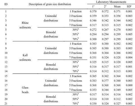
Table 2. Porosity outcomes attained from laboratory measurements and simulations(a, standard deviation; b,
ID Description of grain size distribution Laboratory Measurements
1# 2# Mean SDa
1
Rhine
sediments
Unimodal
distributions
1 Fraction 0.370 0.372 0.371 0.001
2 3 Fractions 0.359 0.353 0.356 0.003
3 5 Fractions 0.346 0.342 0.344 0.002
4 7 Fractions 0.317 0.313 0.315 0.002
5
Bimodal
distributions
30%b 0.272 0.267 0.270 0.003
6 50%b 0.284 0.294 0.289 0.005
7 70%b 0.300 0.297 0.299 0.002
8
Kall
sediments
Unimodal
distributions
1 Fraction 0.383 0.380 0.382 0.002
9 3 Fractions 0.385 0.380 0.383 0.003
10 5 Fractions 0.368 0.364 0.366 0.002
11 7 Fractions 0.331 0.324 0.328 0.004
12
Bimodal
distributions
30%b 0.325 0.315 0.320 0.005
13 50%b 0.316 0.317 0.317 0.001
14 70%b 0.314 0.312 0.313 0.001
15
Glass
beads
Unimodal
distributions
1 Fraction 0.365 0.362 0.364 0.002
16 3 Fractions 0.383 0.377 0.380 0.003
17 5 Fractions 0.368 0.368 0.368 0.000
18 7 Fractions 0.353 0.344 0.349 0.005
19
Bimodal
distributions
30%b 0.317 0.314 0.316 0.002
20 50%b 0.314 0.310 0.312 0.002
21 70%b 0.330 0.324 0.327 0.003
[image:27.595.117.587.294.664.2]27
Table 3. Simulated porosity with varied rebounding probabilities (a, standard deviation)
ID Rebounding
Probability Addition Rate Extra Timesteps Windup Timesteps Simulated porosity
Amount Every
Timesteps
Normal
Timesteps 1
#
2# 3# Mean SD
1 0.1 1 10 7500 0 500 0.437 0.440 0.441 0.439 0.
2 0.2 1 10 7500 0 500 0.433 0.436 0.436 0.435 0.
3 0.3 1 10 7500 0 500 0.434 0.429 0.432 0.432 0.
4 0.4 1 10 7500 0 500 0.434 0.429 0.430 0.431 0.
5 0.5 1 10 7500 0 500 0.434 0.438 0.434 0.435 0.
6 0.6 1 10 7500 0 500 0.433 0.433 0.438 0.435 0.
7 0.7 1 10 7500 0 500 0.446 0.447 0.443 0.445 0.
[image:28.595.121.596.281.408.2]590
Table 4. Simulated porosity with varied addition rates (a, standard deviation)
ID Rebounding
Probability Addition Rate Extra Timesteps Windup Timesteps Simulated porosity
Amount Every
Timesteps
Normal
Timesteps 1
# 2# 3# Mean SD
1 0.25 1 2 1500 0 500 0.460 0.463 0.457 0.460 0.
2 0.25 1 5 3750 0 500 0.446 0.448 0.441 0.445 0.
3 0.25 1 10 7500 0 500 0.434 0.432 0.434 0.433 0.
4 0.25 1 20 15000 0 500 0.424 0.427 0.428 0.427 0.
5 0.25 1 30 22500 0 500 0.423 0.421 0.422 0.422 0.
6 0.25 1 40 30000 0 500 0.421 0.421 0.420 0.421 0.
7 0.25 1 50 37500 0 500 0.420 0.420 0.421 0.420 0.
591
Table 5. Simulated porosity with varied windup timesteps (a, standard deviation)
ID Rebounding
Probability Addition Rate Extra Timesteps Windup Timesteps Simulated porosity
Amount Every
Timesteps
Normal
Timesteps 1
# 2# 3# Mean SD
1 0.25 1 10 7500 500 0 0.434 0.435 0.437 0.435 0.
2 0.25 1 10 7500 500 1000 0.432 0.432 0.434 0.433 0.
3 0.25 1 10 7500 500 2000 0.434 0.431 0.433 0.433 0.
4 0.25 1 10 7500 500 4000 0.435 0.432 0.435 0.434 0.
5 0.25 1 10 7500 500 8000 0.432 0.434 0.432 0.432 0.
6 0.25 1 10 7500 500 16000 0.434 0.433 0.436 0.435 0.
7 0.25 1 10 7500 500 32000 0.431 0.432 0.430 0.431 0.
592 593
[image:28.595.119.596.449.577.2]28
2 4 8 16 32 0
50 100
Grain size (mm)
2 4 8 16 32 0
20 40 60
Grain size (mm)
2 4 8 16 32 0
20 40
Grain size (mm)
2 4 8 16 32 0
10 20 30
Grain size (mm)
2 4 8 16 32 0
10 20 30
Grain size (mm)
2 4 8 16 32 0
10 20 30
Grain size (mm)
2 4 8 16 32 0
10 20 30
Grain size (mm)
Pe
rce
n
ta
g
e
(%
)
Pe
rce
n
ta
g
e
(%
)
A B C D
E F G
595
Fig.1
596
29 598
B
10mm
A
599 600
Fig.2
601
30 0.0 0.2 0.4 0.6 0.8 1.0 0.0
0.2 0.4 0.6 0.8 1.0
Flatness ratio (c/b)
E
lo
n
g
a
ti
o
n
r
a
ti
o
(
b
/a
)
A
Sphere
Rod Blade
Disk
0.0 0.2 0.4 0.6 0.8 1.0 0.0
0.2 0.4 0.6 0.8 1.0
Flatness ratio (c/b)
E
lo
n
g
a
ti
o
n
r
a
ti
o
(
b
/a
)
B
Disk
Rod Blade
Sphere
603
Fig.3
604
31
Glass Rhine Kall
0.0 0.4 0.8
0.2 0.3 0.4 0.5
A
Logarithmic SD (-)
P
o
ro
s
it
y
(
-)
Unimodal
20 40 60 80
0.2 0.3 0.4 0.5
B
Fine mode (%)
P
o
ro
s
it
y
(
-)
Bimodal
606
Fig.4
607
32
300 400 500 600 700 800 900
0.00 0.04 0.08 0.12 0.16
Distance from the River Rhine origin (km)
P
o
ro
s
it
y
d
if
fe
re
n
c
e
(
-)
609
Fig.5
610
33
2 . 8 -4 mm 4 -5 . 6 mm 5 . 6 -8 mm 8 -1 1 . 2 mm 1 1 . 2 -1 6 mm 1 6 -2 2 . 4 mm 2 2 .
A
C B
612
Fig.6
613
34 615
Measured Simulated
20 40 60 80
0.2 0.3 0.4 0.5
F
Fine mode (%)
P o ro s it y ( -) Glass bimodal
0.0 0.4 0.8
0.2 0.3 0.4 0.5
E
Logarithmic SD (-)
P o ro s it y ( -) Glass unimodal
0.0 0.4 0.8
0.2 0.3 0.4 0.5 C P o ro s it y ( -) Kall unimodal
20 40 60 80
0.2 0.3 0.4 0.5 D P o ro s it y ( -) Kall bimodal
0.0 0.4 0.8
0.2 0.3 0.4 0.5 P o ro s it y ( -)
A Rhine unimodal
20 40 60 80
0.2 0.3 0.4 0.5 B P o ro s it y ( -) Rhine bimodal
A Rhine unimodal
R2=0.81 R2=0.82 R2=0.82
R2=0.98 R2=0.94
R2=0.99
616
Fig.7
617
35
G R K
0.2 0.3 0.4 0.5
A
Particle source (-)
G R K
0.2 0.3 0.4 0.5
Particle source (-) B
G R K
0.2 0.3 0.4 0.5
C
Particle source (-)
G R K
0.2 0.3 0.4 0.5
D
Particle source (-)
G R K
0.2 0.3 0.4 0.5
E
Particle source (-)
G R K
0.2 0.3 0.4 0.5
Particle source (-) F
G R K
0.2 0.3 0.4 0.5
G
Particle source (-)
G R K
Measured
Simulated
Porosity (-)
Porosity (-)
619
Fig.8
620
36
Glass Rhine Kall
0.0 0.4 0.8
0 10 20 30 40 50
A
Logarithmic SD (-)
R
e
la
ti
v
e
e
rr
o
r
(%
) Unimodal
20 40 60 80
0 10 20 30 40 50
B
Fine mode (%)
R
e
la
ti
v
e
e
rr
o
r
(%
) Bimodal
622
Fig.9
623
37
2 . 8 -4 mm 4 -5 . 6 mm 5 . 6 -8 mm 8 -1 1 . 2 mm 1 1 . 2 -1 6 mm 1 6 -2 2 . 4 mm 2 2 . 4 -3
A
C B
625
Fig.10
626
38
0.0 0.2 0.4 0.6 0.8
0.41 0.43 0.45 0.47
Rebounding probability (-)
P
o
ro
s
it
y
(
-)
A
0 10,000 20,000 30,000
0.41 0.43 0.45 0.47
Windup timesteps (-)
P
o
ro
s
it
y
(
-)
C
0 1/10 1/20 1/30 1/40 1/50
0.41 0.43 0.45 0.47
B
Addition rate (particle number/timesteps)
P
o
ro
s
it
y
(
-)
39
Fig.11
629