Imaging of gas-liquid annular flows for underbalanced drilling using electrical resistance tomography

Imaging of gas

–

liquid annular

fl

ows for underbalanced drilling using

electrical resistance tomography

Wei Na

a,n

, Jiabin Jia

b,1

, Xin Yu

a

, Yousef Faraj

b

, Qiang Wang

b

, Ying-feng Meng

a

, Mi Wang

b

,

Wantong Sun

a

a

Sate Key Laboratory of O&G Reservoir Geology and Exploitation, Southwest Petroleum University, China b

School of Process and Chemical Engineering, University of Leeds, LS2 9JT, UK

a r t i c l e i n f o

Article history:

Received 10 November 2014 Received in revised form 23 June 2015

Accepted 18 July 2015 Available online 21 July 2015

Keywords:

Underbalanced drilling technique Annularflow

Flow regime

Electrical resistance tomography Flow regime visualisation

a b s t r a c t

The underbalanced drilling technique, which is also known as managed-pressure drilling, is playing an important role in oil and gas sector, as it reduces common conventional drilling problems such as minimal drilling rates and formation damage, differential sticking and lost circulation. Flow regime monitoring is one of the key topics in annular multiphaseflow research, particularly for underbalanced drilling technique. Prediction of the prevailingflow regime in an annulus is of particular importance in the design and installation of underbalanced drilling facilities. Especially, for establishing a suitable pressure-drop model based on the characteristics of the activeflow regime. The methods offlow regime prediction (or visualisation) in an annulus that are currently in use are very limited, this is evidently due to poor accuracy or they are simply not applicable to underbalanced drilling operation in practice. Therefore, this paper presents a monitoring method, in which Electrical Resistance Tomography (ERT) is used to rapidly image the prevailingflow regime in an annulus with a metallic inner pipe. Experiments were carried out using an air–waterflow loop with a test section 50 mm diameterflow pipe. The two-phase air–waterflow regimes are visualised in the upward vertical annulus with a radius ratio (r/R) 0.4. This paper highlights the visualisation results of only threeflow regimes, namely bubbleflow, transi-tional bubble-slugflow and slugflow. Theflow regimes are visualised through axial images stacked from 50 mm diameter-pixels of 2D tomograms reconstructed with the Conjugate Gradient Method (SCG). Gas volume fraction profiles within the annularflow channel are also illustrated. The profiles are extracted using the Modified Sensitivity coefficient Back-Projection (MSBP) method with a sensitivity matrix generated from a realstic phantom in thefinite element method software. The results are compared with visual observations (e.g. photographs) of the activeflow regime at the time of ERT measurements.

&2015 The Authors. Published by Elsevier Ltd. This is an open access article under the CC BY-NC-ND license (http://creativecommons.org/licenses/by-nc-nd/4.0/).

1. Introduction

The growing number of reservoirs around the world and the need for recovering hydrocarbons more efficiently and effectively has been the driving force for oil and gas industry to continuously improve the drilling process. A variety of drilling techniques have been investigated and many of them are currently used in oil and gas industry. One of such techniques is called Underbalanced drilling (UBD), which allows drilling a well more economically, efficiently and safely [15]. The UBD is the process, in which the

wellbore pressure is deliberately designed to be lower than the process of the formation that is drilled. The underbalanced pres-sure conditions facilitate the reservoirfluids to enter the wellbore during drilling, thus preventing fluid loss and related causes to formation damage [2]. In order to achieve UBD conditions, a si-multaneous injection of a mixture of two-phase liquid and gas is required. The two-phase mixture is directly injected into the drill string at the surface, and then the returningfluid isflowing back in an upward vertical fashion in the annulus, outside the drill string [18]. The liquid–gas mixture flows in the annulus according to several topological configurations, which are calledflow regimes, these are namely bubbleflow, slugflow, churnflow and annular flow [7]. Prediction and monitoring these flow regimes are of particular importance for optimisation, diagnostics and control of the process, especially for establishing a suitable pressure drop model in an annulus. As reported in literature that an accurate Contents lists available atScienceDirect

journal homepage:www.elsevier.com/locate/flowmeasinst

Flow Measurement and Instrumentation

http://dx.doi.org/10.1016/j.flowmeasinst.2015.07.003

0955-5986/&2015 The Authors. Published by Elsevier Ltd. This is an open access article under the CC BY-NC-ND license (http://creativecommons.org/licenses/by-nc-nd/4.0/).

n_{Corresponding author.}

E-mail addresses:[email protected](W. Na),

[email protected](M. Wang).

1

down-hole are very different. Therefore, the calculation of multi-phaseflows with the existing multiphaseflow theories deviates from the actual values[8].

Over the years, the researchers have managed to develop some flow regime transition models for annular geometry. However, the prediction accuracy of these models is questionable when they are checked with additional experimental data, particularly when the flow regime is slug or churn. Moreover, a wide range of mea-surement techniques have been reported, so as to provide phase distribution information within an annulus, hence facilitating the design of the processes and visualisation of_flow structure, parti-cularly in drilling wells.[13] used conductivity probes for direct analysis offlow behaviour in vertical annularflow. Their visuali-sation method is quite straightforward, however, it is associated with a major limitation that it does not provide visual observation of the whole pipe cross section; in addition the transparency of the pipe wall is also a major issue. Therefore, in order to provide a clear structure offlow and visualise phase distribution within an opaque annulus, an Electrical Resistance Tomography is a pro-mising technique to non-invasively and rapidly image the internal structure of an annular _flow. Recently, a non-linear ERT re-construction algorithm has been proposed for reconstructing phase distribution within an annulus [17]. They concluded that using ERT, with their developed algorithm, can provide a valuable tool to interrogate the internal structure of an annularflow.

ERT is an imaging technique that can capture the internal structure of a two-phase flow within an opaque pipe or vessel [21,23,24]. The principle of ERT is based on the difference in the conductivity of the constituent phases within multiphase flow domain. It has been successfully applied on many industrial pro-cesses, such as mixing, multiphase flow and so on. The basic principle of ERT operation is that theflow process is interrogated by an array of electrodes (typically 16 electrodes) at the periphery of the pipe wall. An electrical current is injected through a pair of electrodes and the voltage is measured through the remaining electrodes. The main advantage of ERT is that non-intrusive, re-latively inexpensive, fast and safe. Therefore, it can provide a un-ique opportunity to visualise the internal structure of a two-phase flow in an annulus.

A good agreement between results from ERT and a mesh sensor for air volume fraction measurement of air-water upwardflows was reported in our previous work[4]. This study mainly presents an online visualisation technique, in which ERT is utilised to ra-pidly image the internal structure of co-current gas–liquid vertical flow. A corrected sensitivity map and the conjugate gradient method (SCG)[20]with an annularfinite element mesh is used, to offer an effective way of visualising multiphaseflow in an opaque annulus with high pressure and providing a 2- or 3-D spatial and temporal distribution of each constituent phase. In addition, gas volume fraction profiles in an annulus are also measured using Modified Sensitivity coefficient Back-Projection (MSBP) method.

between the sensitivity matrixSand the conductivity changeon one or more areaswithin the sensing domain, as the conductivity change is much smaller than the base conductivity (Eq.(1)) . The image reconstruction is the process of inversely computing the conductivity change vector

Δ

r with known boundary voltage vector

Δ

Vand sensitivity matrixS.The elementary description of vector multiplication for the jth_{voltage change is given as,}

V s 1 j k K j,k k 1

∑

σ

Δ = ⋅Δ

( ) =

wherej¼1, 2,⋯,Jandk¼1, 2,⋯,K;JandKdenote the maximum number of independent voltage measurements on boundary electrode pairs (104 in the case of 16 electrodes per ERT sensor) and the total number of pixels on the 2-dimensional imaging domainak, respectively.

At a pixelkof sensing domain with a homogenous base con-ductivity, the elementaryjth sensitivity coefficient of the sensi-tivity matrix for a current-driven electrode pairmand a voltage measurement electrode pairnis given by Eq.(2)below.

s

I I da 2

j k

a _{m n} k

, m n

k

∫

= − ▿Ф ⋅▿Ψ

( )

where,

Ф

mand,Ψmare potential gradients over pixelakdue to current-driven electrode pairmandnrespectively. The integration is made over the area of pixelk. The sensitivity matrixSis a j×k

matrix, which is composed from the sensitivity coefficient over the whole sensing domain A.

The recent research work found that based on the nonlinear approximation, the modified sensitivity back-projection (MSBP) method as expressed in Eq. (3) [19,20] is a more accurate ap-proximation than the traditional linear back-projection method[9] to obtain thekth conductivity ratiosk/s1[6].

s s 3 k j J k j j J k j V V 1 1 ,

1 , j

j σ σ ≈ ∑ ∑ ⋅ ( ) = = ‵

wheresk,jis an element of the transpose matrix of the sensitivity matrixS, Vjis the jth baseline voltage measured on ERT sensor containing only single continuous phase with conductivitys1, and V‵jis the jth voltage measured on ERT sensor after two phase mixture presents and conductivity is altered tosk.

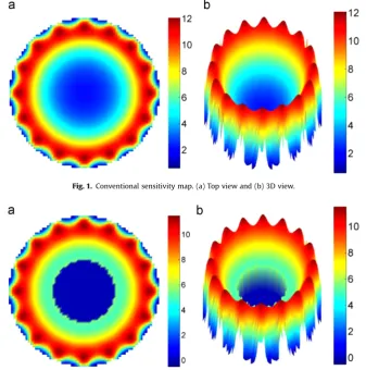
The Finite Element Method (FEM) software like COMSOL can simulate this process and compute the sensitivity map. Fig. 1 graphically shows the sensitivity map of a conventional circular ERT sensor with adjacent sensing strategy. The 3D view ofFig. 1 (b) demonstrates that in the circular sensing domain, the periph-eral area is more sensitive to the conductivity change than the central area.

using ERT imaging technique. In the experiment, the diameter of theflow pipe is 50 mm. A steel pipe with 20 mm diameter is in-serted at the centre of the pipe. Rather than using conventional sensitivity matrix ofFig. 1, a realistic phantom in the FEM software should be built to compute the unique sensitivity matrix for ERT image reconstruction. Since the metallic pipe provides an equi-potential to the inner wall of the annulus, as shown in Fig. 2, electricalfield (V/m) abruptly drops to zero within the region of the solid steel pipe, which will lead to constant grey column on reconstructed ERT images as given inSection 4.

A new meshfile was generated with corresponding boundary conditions for a 192 elements and 141 nodesfinite element mesh

as shown in Fig. 3(a). Typical images reconstructed with SCG method are illustrated byFig. 3(b) and (c) in correspondence to flow conditions of bubbleflow (Vsa¼0.085 m/s,Vsw¼1.039 m/s) and slugflow (Vsa¼0.425 m/s,Vsw¼0.342 m/s).

2.2 Correlation between conductivity and volume fraction

[image:3.595.141.466.58.221.2]

ERT produces not only images with respect to conductivity distribution, but the local and overall volume fraction of dispersed phase in the two-phase _flow. The Maxwell relationship[11] for-mulated in Eq.(4)with the zero conductivity of particles is mostly used to correlate thekth local gas volume fractionckover pixelak Fig. 1.Conventional sensitivity map. (a) Top view and (b) 3D view.

[image:3.595.133.471.59.400.2]

Fig. 2.Unique sensitivity map. (a) Top view and (b) 3D view.

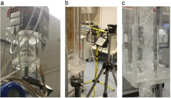
[image:3.595.58.544.566.731.2]

A set of tests were carried out using the non-pressurised multiphase flow facility at the University of Leeds. A schematic diagram of theflow facility is illustrated inFig. 4. The pipeline is of Plexiglas with 50 mm internal diameter and 5 mm wall thickness. Air and tap water was used at room temperature. Theflow loop facilitates separate injection of water and air at the horizontal section and eventually mixed up after the loop bend, where the mixture of water and air is introduced to the vertical upwardflow test section. The injection of air and water into theflow loop is highlighted by different coloured lines inFig. 4. The water injec-tion stream is presented by a blue line; air injecinjec-tion stream is presented by a red line, while the green line denotes the mixture of air and waterflow. The loop is an open recirculatingflow loop. This means that after injecting air and water, the mixture goes through the vertical test section and returned to a holding tank through a horizontal returning limb (5.8 m length). The air is re-leased into the atmosphere at the discharge point, while water is returned into the tank and reintroduced into the flow loop. The recycled water is reintroduced into the loop through a jet pump, which connects the downstream of the loop to the water tank. The inlet waterflow rate is controlled through a ball valve and mea-sured using a water turbineflow meter (Omega). The inlet airflow rate is controlled through a gas mass flow controller (Omega FMA5542, 0-100 Standard Litre per Minute (SLPM)).

transducers and the temperature sensor, which are used to monitor theflow conditions, are mounted at the two ends of the test section.

[image:4.595.133.456.484.736.2]

Due to the limitation in the capability of theflow loop, only two flow regimes can be created, bubbleflow and slugflow, which may not correspond the developedflow regime due to the limitedflow rising length Nevertheless, the exact formation offlow regime is not the focus of this study, as previously mentioned that the main aim of this study is to present a monitoring method for rapidly imaging the prevailingflow regime in an annulus. Therefore, the experimental_flow conditions were designed to cover these two flow regimes, along with the transitionalflow regime from bubble flow to slug flow. The range of airflow rate used in the experi-ments was 10–60 SLPM (0.085–0.509 m/s superficial air velocity), while the range of waterflow rate was 20–145 RPM (Rotation per Minute) (0.209–1.039 m/s superficial water velocity). The experi-mentalflow conditions were split into three sets of conditions in terms of gasflow rate; Low gasflow rate (10–20 SLPM) to produce bubbleflow regime, medium gasflow rate (30–50 SLPM) to pro-duce bubble, slug and transitionalflow regime, while high gas flow rate (60 SLPM) to give slug_flow and transitional_flow regime. The ERT measurements, at each flow condition, were carried out, along with capturing photographs of the mixture flow through the cross-section of the annulus for latter evaluation of

the ERT visualisation method. A high performance ERT measure-ment system (Fast Impedance Camera System-FICA or z8000)[22] was used to measure the flow of the mixture and capture the image of the cross-section of the annulus. The FICA system is an high performance ERT system, which is capable of acquiring 1000 dual frames per second. Each measurement data is averaged, through which the local air volume fraction profile is produced. The local air volume fraction is determined from the conductivity data using Maxwell relationship [11]formulated in Eq. (4). The ERT in principle measures the relative voltage difference between continuous flow (water) and mixture flow (air and water). This then used to calculate the local conductivity of each pixel located within the annulus region. The MSBP method described in Section 2.1 is used to convert the relative voltage difference to con-ductivity distribution (maps) of the cross-section of annulus under investigation. Based on the new sensitivity map generated in Section 2.1, the Sensitivity theorem based inverse solution using Conjugate Gradient (SCG) method[20]was used to reconstruct the off-line images of eachflow condition. The reconstructed cross-sectional image shows annular area of air–waterflow and solid steel rod.

4. Experimental results and discussion

All the ERT measurement data obtained from ERT (z8000 or FICA) system for eachflow condition was collected and entered into P2000 software to produce the conductivity map and re-constructed image of the annular flow region. Eachflow image was reconstructed using the SBP method with an improved sen-sitivity map, through which only the annular area was taken into account and the pixels, fall into the boundary of the inner pipe, are excluded. The conductivity map inverted was then imported into the software AIMFlow (Advanced Imaging and Measurement for Multiphaseflow) to generate the tomograms of the annular re-gion. The tomograms reconstructed for eachflow condition were collected and analysed, so as to produce images of the annulus and to determine the local air volume fraction (void fraction). The cross-sectional image (or the tomogram) provides valuable in-formation over the dynamic behaviour of each phase within the pipe and can readily be used for the purpose of visualisation. However, for detailed qualitative evaluation and visualisation, the air volume fraction profile may be more useful to visualise the internal structure of annular_flow. Apart from the pro_files, axial stacked images reconstructed using SCG were also produced,

through which the dynamic of air and water can be visualised along the annulus section. 1000 frames (tomograms) generated by each plane were processed through an in house developed pro-gram to generate the stacked images. The propro-gram uses the se-lected nodes from each plane (mesh) and generates a text matrix, on which the final stacked images are based. The generated stacked images are illustrated below. In order to evaluate the vi-sualisation scheme, the results obtained from the ERT are com-pared with visual observations (photograph), as discussed below.

For simplicity, only three conditions are selected and discussed in this paper. The selected conditions are bubbleflow, which re-presentative of low gasflow rate; transitional regime, which re-presentative of medium gasflow rate and slugflow, which falls into the category of high gas flow rate. Figs. 6–8 show the test results, in which present (a) photographs; (b) stacked 1000 to-mograms reconstructed with SCG algorithm (c) gas volume frac-tion profiles. Each stacked image has its individual colour range to visualise gas_–liquid distribution.

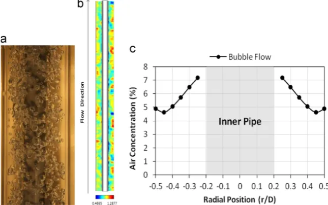
[image:5.595.140.466.58.245.2]

and evaluation of the image within the pipe. By observing the stacked images of air and waterflow along the annulus, a sym-metrical distribution of air and water can be seen across the cross-section of the annulus. It is also clear that the bubblesflow closer to the inner pipe wall, as it is suggested by the visual observation. It can also be seen that the profile slightly goes down close to the outer pipe wall, and then the peak takes on again. This could be attributed to the limitations associated with the sensitivity map, which is used for image reconstruction.

Fig. 7shows the concentric annular transitionalflow pattern from bubbleflow to slugflow. Once the airflow rate increased from 10 SLPM (0.085 m/s air superficial velocity) to 30 SLPM (0.225 m/s air superficial velocity) and the water flow rate de-creased from 145 RPM (1.039 m/s water superficial velocity) to 60 RPM (0.475 m/s water superficial velocity) it was noticed through visual observation that theflow of bubbles through the cross-section of the annulus had almost similar characteristics to thoseflow in a circular full bore pipe. With the increase of airflow rate the number of bubbles increase and move as packed bubbles. This leads to the increase of air density within the annulus region.

With the increase of density it is apparent that the bubblesflow faster in upward vertical section in a zig-zag fashion but inter-leaved with large bubbles. The higher number of bubbles in the flowing media and their faster movement increases the rate of collision and rate of agglomeration among the packed bubbles. As a result, larger bubbles are formed occasionally, which eventually leads to slug flow if the air flow rate is further increased. This phenomenon can be noticed in the visual observation inFig. 7(a). Similar to bubble low, the highest air volume fraction can be seen close to the inner pipe wall. The movement and distribution of each phase, air and water, is clearly highlighted in the stacked images shown inFig. 7(b). By comparing the staked images with the visual observation, a reasonably accurate representation of flow shown in the visual observation can be noticed. With regard to the gas volume fraction profile, it is apparent that highest air volume fraction is again present close to the inner pipe wall, which well agrees with the visual observation (photograph).

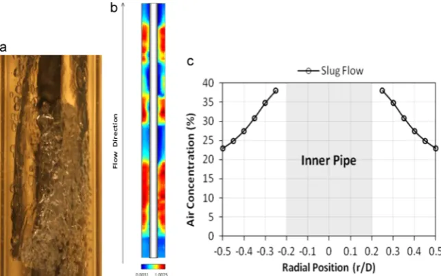
[image:6.595.130.453.60.262.2] [image:6.595.131.453.520.724.2]

In slugflow, as it is shown inFig. 8, the airflow rate is 50 SLPM (0.425 m/s air superficial velocity) and waterflow rate is 40 RPM (0.342 m/s water super_ficial velocity). Similar trend can be Fig. 6.Concentric annular bubbleflow (Vsa¼0.085 m/s,Vsw¼1.039 m/s) (a) visual observation, (b) Stacked 1000 images of the mixture along axial section of the annulus, and (c) volume fraction profile. (For interpretation of the references to color in thisfigure, the reader is referred to the web version of this article.)

observed as that of bubbleflow and transitionalflow regime. The air phase has a tendency offlowing closer to the inner pipe wall, similar to that of bubble and transitional regime. The range of air volume fraction within the annulus is shown by the volume fraction profile as approximately 23–37%. The highest air volume fraction can be seen close to the inner pipe wall in both, the visual observation and air volume fraction profile. This phenomenon is also suggested by the stacked images of the flowing mixture within the pipe annulus, shown inFig. 8(b). It can be seen that the airflows as large bubbles. The shape of large bubbles present in the annulus region is noticeably different to thatflowing in a cir-cular full bore pipe. The shape of larger bubblesflowing through the annulus is somehow elongated and moving in an asymme-trical fashion. Some dispersed bubbles can also be seen, which are carried by the liquid in the area close to the outer pipe wall. These dispersed bubbles are formed as a result of collision of water with larger bubbles as the water falls downward into the region that is not occupied by the larger bubbles.

The mean air volume fraction obtained from ERT across the cross-section of the annulus, and mean air volume fraction based on inletflow conditions are shown inTable 1. It is worth pointing out that the inlet air volume fraction is determined based on standard conditions (1.01 bar and 21.1°C). It is quite apparent that the air volume fractions at standard conditions can be converted to actual volume fraction (at loop temperature and pressure) for the purpose of comparison and evaluation of the measured values. However, as the main focus of this work is merely onflow visua-lisation rather thanflow metering, the evaluation of measured air volume fraction is beyond the scope of this paper. Therefore, the results highlighted inTable 1, are only an indication of ERT mea-sured mean air volume fractions against their respective inlet volume fractions.

5. Conclusions

A high performance ERT technique is proposed for visualisation of two-phase gas_–liquid_flow in an annulus with a metallic inner pipe. The ERT using a revised sensitivity map and a meshfile with corresponding boundary conditions is used to interrogate the in-ternal structure of annularflow for bubble, transitional and slug flows. Axialflow regimes are compared with visual observations. Although tomographic images cannot be as clear as the photo-graphs captured during the measurements, ERT is still able to provide enough information regarding the prevailingflow regime within the annulus. The air volume fraction profiles in the annulus region, produced from the ERT, indicate a good agreement be-tween the profiles and visual observation (photographs). The stacked images are reasonably accurate representation of air water in the annulus region for the conditions used in this study. Further work will be carried out to evaluate gas_flow pro_files with other references.

Acknowledgement

The research was supported by the Open Fund of State Key Laboratory of Oil and Gas Geology and Exploration at Southwest Petroleum University (PLN1119), National Natural Science Foun-dation of China (51204140, L1322021 and 51334003). Authors would like to thank Mr. Yunjie Yang for preparing thefigures of the sensitivity matrix.

References

[1]D.C. Barber, B. Brown, Applied potential tomography, J. Phys. E: Sci. Instrum. 17 (1984) 723–733.

[2]Bourgoyne Jr., T. Adam, Rotating control head applications increasing, Oil Gas J. (1995) 72.

[3]S. Ghosh, D.K. Pratihar, B. Maiti, P.K. Das, Automatic classification of vertical counter-current two-phaseflow by capturing hydrodynamic characteristics through objective descriptions, Int. J. Multiph. Flow 52 (2013) 102–120. [4]C. Olerni, J. Jia, M. Wang, Measurement of air distribution and void fraction of

an upwards air–waterflow using electrical resistance tomography and a wire-mesh sensor, Meas. Sci. Technol. 24 (3) (2013) 1–9.

[5]P.J. Holden, M. Wang, R. Mann, F.J. Dickin, R.B. Edwards, Imaging stirred-vessel macromixing using electrical resistance tomography, Am. Inst. Chem. Eng. J. 44 (4) (1998) 780–790.

[image:7.595.141.463.57.258.2]

[6]J. Jia, M. Wang, Y. Faraj, Evaluation of EIT systems and algorithms for handling Fig. 8.Concentric annular slugflow (Vsa¼0.425 m/s,Vsw¼0.342 m/s) (a) visual observation, (b) Stacked 1000 images of the mixtureflow along axial section of the annulus, and (c) volume fraction profile.

Table 1

Mean air volume fraction across the cross-section of the annulus.

Mean air volume fraction Bubble Transitional (bubble–slug) Slug

ERT 0.06 0.14 0.3

[image:7.595.42.293.321.364.2]

flow boiling of water in a horizontal annulus using high-speedflow visuali-zation, Heat Transf. Eng. 34 (10) (2012) 838–851.

[14]D. Reitsma, R.E. Van, Utilizing an automated annular pressure control system for managed pressure drilling in mature offshore oilfields, J. SPE (2005) 96646. [15] Shale, L.T., 1994. Underbalanced drilling: formation damage control during

high-angle or horizontal drilling. Paper SPE 27351 Presented at the Interna-tional Symposium of Formation Damage Control held in Lafayette, LA,

mance EIT System, IEEE Sens. J. 5 (2) (2005) 289–299.

[23]M. Wang, R. Mann, F.J. Dickin, Electrical resistance tomographic sensing sys-tems for industrial applications, Chem. Eng. Commun., 175, (1999) 49–70. [24]R.A. Williams, X. Jia, R.M. West, M. Wang, J.C. Cullivan, J. Bond, I. Faulks,