White Rose Research Online URL for this paper:
http://eprints.whiterose.ac.uk/95784/
Version: Submitted Version
Article:
Cowtan, Kevin orcid.org/0000-0002-0189-1437 and Way, Robert G. (2014) Coverage bias
in the HadCRUT4 temperature series and its impact on recent temperature trends.
Quarterly Journal of the Royal Meteorological Society. pp. 1935-1944. ISSN 0035-9009
https://doi.org/10.1002/qj.2297
[email protected] https://eprints.whiterose.ac.uk/ Reuse
Items deposited in White Rose Research Online are protected by copyright, with all rights reserved unless indicated otherwise. They may be downloaded and/or printed for private study, or other acts as permitted by national copyright laws. The publisher or other rights holders may allow further reproduction and re-use of the full text version. This is indicated by the licence information on the White Rose Research Online record for the item.
Takedown
If you consider content in White Rose Research Online to be in breach of UK law, please notify us by
Coverage bias in the HadCRUT4 temperature series and its
impact on recent temperature trends.
Kevin Cowtan
a∗Robert Way
baDepartment of Chemistry, University of York, UK
bDepartment of Geography, Memorial University of Newfoundland, Canada
∗Correspondence to: [email protected]
Incomplete global coverage is a potential source of bias in global temperature reconstructions if the unsampled regions are not uniformly distributed over the planet’s surface. The widely used HadCRUT4 dataset covers on average about 84% of the globe over recent decades, with the unsampled regions being concentrated at the poles and over Africa. Three existing reconstructions with near-global coverage are examined, each suggesting that HadCRUT4 is subject to significant bias due to its treatment of unobserved regions.
Two alternative approaches for reconstructing global temperatures are explored, one based on an optimal interpolation algorithm and the other a hybrid method incorporating additional information from the satellite temperature record. The methods are validated on the basis of their skill at reconstructing omitted sets of observations. Both methods provide superior results than excluding the unsampled regions, with the hybrid method showing particular skill around the regions where no observations are available.
Temperature trends are compared for the hybrid global temperature reconstruction and the raw HadCRUT4 data. The widely quoted trend since 1997 in the hybrid global reconstruction is two and a half times greater than the corresponding trend in the coverage-biased HadCRUT4 data. The impact of coverage bias in the HadCRUT4 data leads to an overestimation of global temperature during the late-1990s and an underestimation of global temperatures over the past decade. Trends starting in 1997 or 1998 are therefore maximally misleading with respect to the global trend. The issue is exacerbated by the strong El Ni ˜no event of 1997-1998, which also tends to suppress trends starting during those years. Copyright c0000 Royal Meteorological Society
1. Introduction
The instrumental temperature record, based on land-based
weather station readings and sea surface temperature
readings from ships and buoys, forms a vital source of
information concerning climate over the last century and
beyond. Time series of local monthly average temperatures
(gridded datasets) and global averages are produced by
several organisations, with the HadCRUT product of the
Hadley Center and Climatic Research Unit being one of
the most widely cited (Moriceet al.2012). The GISTEMP
product from NASA’s Goddard institute (Hansen et al.
2010) and the NCDC product (Smithet al.2008) are also
widely used. A new land-only product from the Berkeley
Earth ‘BEST’ project (Mulleret al.2012) has introduced a
number of statistical improvements in the handling of data
homogenisation and coverage.
All these temperature reconstructions are based on in
situ readings using thermometers. While the production
and calibration of reliable thermometers has been well
established for several centuries, how the thermometers
are used to obtain meteorological data can significantly
influence the results. The introduction of the Stevenson
screen provided a significant step towards the collection of
reliable air temperature data from land stations, however
some biases remain in both the land and sea surface
temperature data.
Most of the biases have been studied at length
and addressed by both data-only approaches (i.e. using
just the temperature observations) and meta-data based
approaches (i.e. including additional information such as
time of observation and measurement methodology, see
for example Peterson and Vose 1997). The most widely
studied sources of measurement bias in the land temperature
record are the time of observation (Karl et al. 1986),
instrumentation type, and the ‘Urban Heat Island’ (UHI)
effect (Hausfatheret al.2013).
Two recent results are particularly noteworthy. A
comprehensive study of US stations by Williams et al.
(2012) compared pairs of stations and correlated differences
in the data with metadata analysis to conclude that time of
observation and instrumentation location and type were the
principal sources of bias in the weather station data. The
BEST analysis (Muller et al. 2012) addresses these two
source of bias in a different way, using a data-only approach
to divide each station record into segments which show no
discontinuity with respect to consensus local climatology.
The agreement between the data-only approach of BEST
and the metadata based approach of NCDC provides strong
support for the reliability of the resulting record.
Practices for measuring sea surface temperatures have
also changed over time, leading to biases in the
resulting data. Early measurements were performed using
uninsulated buckets to bring sea water on deck, while
more recent measurements have used insulated buckets,
engine room intake temperatures, and anchored or
free-floating buoys (Kennedy et al. 2011). Measurements
using uninsulated buckets tend to be biased cool due to
evaporation from the bucket, while engine room intake
temperatures tend to be biased warm due to heating of
the water by the ship infrastructure. A discontinuity in
the raw temperature record due to a transition from the
use of uninsulated buckets to engine room intakes at the
beginning of the second world war was quantified by
Folland and Parker (1995) and is addressed by a ‘bucket
correction’ in the widely used versions of the instrumental
temperature record. More recently, a second discontinuity
was identified by Thompsonet al. (2008) by comparison
of the instrumental temperature record with climate model
outputs. Kennedy et al. (2011) conducted a detailed
to the SST data, addressing the discontinuity at the end
of WWII. This work also introduced a smaller upward
adjustment to recent temperatures due to a transition away
from warm-biased engine room sensors to measurements by
buoys. These corrections are currently only present in the
Hadley/CRU temperature record (Moriceet al.2012).
Other sources of temperature data include reanalysis
data, which are determined by using a weather model
to reconstruct a global temperature field on the basis
of multiple sources of data (e.g. Kalnay et al. 1996),
and the satellite temperature record (Spencer 1990; Mears
and Wentz 2009). The satellite temperature record is of
particular interest because it provides a uniform sampling
with near-global coverage. However the satellite microwave
sounding units measure lower troposphere rather than
surface temperatures and so are not directly comparable
to the in situ temperature record. Furthermore there
are temporal uncertainties in the satellite record arising
from satellite failure and replacement and the numerous
corrections required to construct a homogeneous record.
Contamination of the microwave signal from different
surface types is also an issue, particularly over ice and at
high altitude (Mearset al.2003).
1.1. Coverage bias
A further important source of bias arises from the estimation
of a global mean temperature from the incompletely
sampled gridded dataset. Weather stations coverage is best
in the temperate latitudes and particularly in developed
nations. Coverage of the polar regions is particularly poor,
with no coverage of Antarctica before the 1950’s, and
limited coverage of the Arctic to this day. Poor sampling
of the fastest warming parts of the planet leads to an
underestimation of the global trend in the instrumental
temperature record (Met Office 2009). This problem is
exacerbated by the use of equal-angle (5 degree) grids by
the Hadley/CRU record (Stokes 2011). Since equal-angle
grid cells become smaller at higher latitudes, more stations
are required to achieve full coverage when in practice fewer
stations are available.
Coverage bias becomes an issue when different parts of
the planet are changing temperature at different rates. As a
result it is a particular issue over recent decades, owing to
the different rates of warming between the tropics and poles,
and between land and ocean (Hansenet al.2006). Changes
in the Arctic and Antarctic are particularly problematic
because the coverage is poor in these regions.
While short term trends are generally treated with a
suitable level of caution by specialists in the field, they
feature significantly in the public discourse on climate
change (e.g. Global Warming Policy Foundation 2012;
Daily Mail 2012; The Telegraph 2013), and have also been
the subject of scholarly studies into the possible impact of
both aerosol emissions (Kaufmannet al.2011) and ocean
heat uptake in climate models (Meehlet al.2011) on short
term trends. A common factor in all these works is an
attempt explain or draw conclusions from the comparatively
slow warming seen in some versions of the instrumental
temperature record over the past decade and a half. However
to do so without first addressing the issue of coverage bias
is to ignore a very significant confounding factor in the
analysis.
NASA’s GISTEMP temperature record (Hansen et al.
2010) attempts to address the coverage issue by
extrapo-lating temperatures into unmeasured regions by means of
kernel smoothing using a conical kernel of radius 1200km.
The Berkeley Earth (BEST) project have adopted an optimal
interpolation method (kriging), although only for land
tem-peratures at this stage (Mulleret al.2012). A recent memo
from this project (Rohde 2013) suggests that the simple
kernel smoothing method used by GISTEMP gives results
these approaches assumes that the unobserved high latitude
temperature field varies in a similar way to the observed
temperatures at lower latitudes.
The potential impact of coverage bias may be estimated
by use of three (near) global temperature reconstructions:
The extrapolated GISTEMP data, the UAH satellite data,
and the NCEP/NCAR reanalysis data (the NCEP/DOE
AMIP-II Reanalysis-2 gives similar results). Figure (1)
shows temperature trend maps for the period
1997/01-2012/12 for HadCRUT4 and each of these three series (the
significance of the start date will become clear shortly).
Note that GISTEMP, UAH and NCEP/NCAR all show
significantly faster warming in the Arctic than over the
planet as a whole, and GISTEMP and NCEP/NCAR also
show faster warming in the Antarctic. Both of these regions
are omitted in the HadCRUT4 data. If the other datasets are
right, this should lead to a cool bias due to coverage in the
HadCRUT4 temperature series.
A preliminary estimate of the size of the bias may be
calculated from the three global temperature series. For each
series the coverage of the temperature field for each month
is reduced to match that of the HadCRUT4 data for that
month. Global mean temperature estimates are calculated
for both the full- and reduced-coverage temperature fields.
The difference between these values gives an estimate of
the coverage bias. The bias estimate can vary dramatically
from month to month as weather systems move in and out of
the omitted regions, however a 60 month moving average,
shown in Figure (2), shows long term variations. All the
global series show a shift from a warm to a cool bias over the
past two decades, with the sharpest decline starting around
1998. The GISTEMP and UAH estimates for HadCRUT4
coverage bias are very similar, providing some support for
the GISTEMP extrapolation approach. The NCEP/NCAR
data show a much faster transition to a cool bias followed by
a plateau, raising a question over the GISTEMP assumption
that temperatures at high latitudes vary similarly to those at
lower latitudes.
The timing of this change in bias after 1998 is significant
because it also corresponds to a strong El Nino event
(leading to a warm year) and is often suggested as the start
of a hiatus in global warming (e.g. Meehl et al. 2011).
However the consensus of the three global temperature
series is that short term trends starting around
1997-1998 will be maximally misleading in the estimation of
underlying trends, because they are distorted by the full
effect of both coverage bias and the strong 1997-1998 El
Nino event.
The purpose of this work is to address the issue of
coverage bias through the development of new methods
for global temperature reconstruction building on the
HadCRUT4 data.
2. Global temperature reconstruction
In order to construct a global surface temperature series,
either surface temperature observations or proxies which
allows their estimation are required. No static weather
station observations are available for the central Arctic,
and thus a proxy is the only option. Hansen et al.
(2006) used the UAH satellite data to argue that a warm
Arctic anomaly responsible for the GISTEMP temperature
record in 2005 was genuine. The satellite data has near
global coverage, and the global distribution of satellite
temperatures for any given month is correlated with the
surface temperatures, with a mean (Pearson) correlation of
0.61between GISTEMP and UAH when using the same
baseline period. Therefore the satellite data will be used as a
proxy for surface temperature to construct a geographically
complete hybrid temperature record.
The UAH satellite data is used in preference to data
from RSS because RSS omits the critical high latitude
contamination issue. This work aims to mitigate surface
contamination bias by use of the in situ data. The UAH
data is also interpolated at latitudes above 85◦, however
the interpolated region is small compared to the unobserved
region of the in situ data.
The use of the satellite temperatures as a proxy rather
than a direct measurement of surface temperature brings
additional requirements. Firstly, the satellite and in situ
observations must be on a common baseline. Secondly, an
appropriate method for mapping satellite observations of
lower troposphere temperatures onto surface temperatures
is required. Thirdly, the method must be validated to ensure
that it has skill in predicting unobserved temperature values.
The validation step will also serve as a check on the possible
issues identified so far such as the mismatch between
surface and lower troposphere temperatures and surface
contamination of the MSU signal.
The mapping and validation steps will make use of
the optimal interpolation algorithm known as kriging. For
the mapping, kriging will be used to estimate a slowly
varying function of grid coordinates corresponding to the
offset between the satellite and surface temperatures. For
the validation step, kriging will provide a baseline against
which to compare the skill of the hybrid method.
2.1. The impact of the baseline period
The surface temperature calculation is usually performed
using temperature anomalies, which represent the deviation
of the current temperature from the mean over a chosen
baseline period. For the HadCRUT4 data, the station data
are normalised so that the mean over the period
1961-1990 for a given month of the year is zero for each station
with sufficient records. The UAH map data uses a similar
approach with the mean for each map cell normalised to
zero over the period 1981-2010 for a given month of the
year.
A problem arises when coverage changes over time.
Because the Arctic has warmed significantly since the
end of the HadCRUT4 baseline period, a drop in Arctic
coverage leads to a cool bias in the mean of the observed
cells. This effect increases as conditions diverge from the
baseline period. To obtain realistic short term trends, the
baseline period should be as similar to the trend period as
possible. For similar reasons, when constructing a hybrid
temperature series, the two source map series should have
the same baseline period.
The HadCRUT4 map series was therefore renormalised
to match the UAH baseline period of 1981-2010. For each
map cell and each month of the year, the mean value of that
cell during the baseline period was determined. If at least 15
of the 30 possible observations were present, an offset was
applied to every value for that cell and month to bring the
mean to zero; otherwise the cell was marked as unobserved
for the whole period.
Renormalization is not a neutral step - coverage is
very slightly reduced, however the impact of changes in
coverage over recent periods is also reduced. Coverage
of the renormalized HadCRUT4 map series is reduced by
about 2%.
2.2. Kriging
Kriging (Cressie 1990) is an linear approach to
interpo-lation/extrapolation in which the values of the field are
determined in accordance with a given covariance structure,
where the covariance structure is usually a radial function
which is determined from the covariance of those
observa-tions which are present. The radial function is usually a
sim-ple function, such as an exponential, although Mulleret al.
(2012) use the exponential of a higher order polynomial.
Kriging is an important method in geophysics, offering
1. The reconstructed values vary smoothly and match
the observed values at the coordinates of the
observations.
2. For well behaved covariance functions the
recon-structed values approach the global mean as the
dis-tance from the nearest observation increases, i.e. the
method is conservative with respect to poor coverage.
3. When a reconstructed value is produced based on
a cluster of observation in one direction and a
single observation in another, the cluster values
are downweighted in accordance with the amount
of independent information they contribute to the
reconstructed value. Area weighting is an emergent
property of the method, with observations being
weighted by cell size in densely sampled regions,
and by the region over which the observation is
informative in sparse regions.
The kriging calculation is described in detail in Appendix
A, however in outline the steps are as follows:
• Determine the radial covariance function from the
observations which are available.
• Construct a covariance matrix for the observed
coordinates.
• Construct a vector of covariances between the
observed coordinates and some coordinate at which
an estimate of the field is desired.
• Solve the resulting system of equations for the to
obtain a vector of weights. The estimated value of
the field at the target coordinate is given by the dot
product of vectors of weights and the observations.
There are differences between the method employed here
and that of Mulleret al.(2012). Mulleret al.used simple
kriging, which assumes that the expectation of the unknown
field is zero - this was a valid approach for that work since
the expectation of the field had already been subtracted out
in the form of a time varying climate term. In this work, the
expectation of the field (i.e. the global mean temperature) is
to be determined so ordinary kriging, which makes no such
assumption, is required. Ordinary kriging introduces an
additional constraint that the weights must sum to unity, and
thus the applying a constant offset to all the observations
leads to a corresponding offset in every extrapolated value.
In this work the kriging calculation will be applied
to the reconstruction of gridded temperature values using
the grid cells for which observations are available, in
contrast to Mulleret al.who use individual stations as the
observations. This will enable a correspondence between
the gridded satellite data and the surface data, and also
makes it computationally realistic to construct a full matrix
of cell covariances rather than the sparse matrix used by
Muller et al., allowing a global reconstruction from any
starting data. In a 5 degree sampled grid there are 2592
cells, and so the correlation matrix can contain up to 8.7m
(25912) elements. The covariance function was modelled
by a simple exponential function of distance, ensuring
a strongly diagonal covariance matrix and a numerically
stable calculation.
Kriging the gridded data also has some significant
disadvantages: Information about station position within a
cell is lost, cells with a single station receive the same
weight as cells with many, and (equivalently) no account is
taken of the uncertainty in a cell value. The acceptability of
these compromises will become apparent in the validation
step.
Grid cells for which observations are available are
assumed to be exact, and are therefore unmodified by the
calculation. This is not a necessary assumption of kriging,
but for the purposes of estimating global mean temperatures
it is a convenient simplification and means that the resulting
temperature fields will preserve the features of the source
2.3. The hybrid calculation
The hybrid surface-satellite temperature calculation is
extremely simple in form:
Thybrid
x = krig(T
surf−sTsat)
x+sTxsat (1)
where Tsurf
x is the surface temperature of the grid cell
at coordinate x, Tsat
x is the satellite temperature, and s
is a scale factor applied to the satellite temperatures. The
difference between the surface and satellite temperatures
may only be calculated for cells where surface temperatures
are available, so the result has incomplete coverage, which
is completed by the kriging operator. The resulting global
coverage field is added to the scaled satellite temperatures
to produce the hybrid temperature field. The scale factor s
serves to allow for a difference in scale between surface and
lower troposphere (LT) temperatures.
The krigged difference field has the following properties:
1. Where a surface temperature observation is present,
it is the difference between the surface and satellite
temperatures.
2. Near a surface temperature observation the value of
the field will be similar to the difference at the nearest
observed coordinate.
3. Far from any surface temperature observation the
value of the field will approach the difference
between the global means of the surface and satellite
fields.
These properties translate to the following properties for
the hybrid field:
1. Where a surface temperature observation is present,
the hybrid field is equal to the surface temperature.
2. Near a surface temperature observation the value
of the field will be similar to the nearest observed
coordinate.
3. Far from any surface temperature observation the
value of the field will approach the value of the
satellite field, adjusted by the difference in global
mean between the surface and satellite fields.
The hybrid field around an isolated surface observation will
match the satellite data in gradient and curvature, with a
constant offset to fit the surface observation at the grid
centre.
In other words the behaviour is what one would
intuitively expect from a hybrid temperature reconstruction,
with the distances over which a surface observation can
dictate local temperatures determined by the autocorrelation
of the difference field itself.
Any temporal inhomogeneity in the satellite data
is eliminated, because the satellite data is tied to
the surface temperature observations on a
month-by-month basis. Spatial inhomogeneity, for example due to
surface contamination of the tropospheric temperature
observations, remains an issue only if inhomogeneity varies
over distances significantly shorter than the range of the
kriging calculation.
2.4. Validation
The satellite data does not provide direct surface
temperature observations, and thus must be treated as a
proxy dataset. Also the kriging calculation implemented
here does not account for uncertainties in the observations,
or even the number of observations in a grid cell. Each
of these factors mean that the method can not be assumed
to be valid, and therefore the skill of the method must be
proven by reconstructing temperature observations which
have been hidden from the calculation. For the following
tests, the HadCRUT4 ensemble median and UAH data
were used over the period 1979/01-2012/12. The UAH
will be employed; the first being a 36-fold cross validation
approach modified to deal with the spatial autocorrelation
of the data.
In the cross validation calculation, a contiguous group
of either 1, 3, or 5 latitude bands are omitted from the
temperature map data for a given month. The central latitude
band of the omitted region is then reconstructed by one of
the following methods:
• Null reconstruction - the target cells are set to the
(area weighted) mean of the rest of the map.
• Kriging - the target cells are reconstructed using the
kriging calculation.
• Hybrid - the target cells are reconstructed using
the hybrid method. This approach is repeated for
different values of the satellite scale factor s.
The calculation is repeated 36 times, omitting the latitude
bands bracketing each of the 36 latitude bands in turn.
The 36 reconstructed bands are then combined to create a
composite map in which every cell has been reconstructed
using only cells more than a certain distance from that cell.
The three extrapolation ranges are illustrated in Figure (3).
The skill of the temperature reconstruction methods may
be measured in terms of the RMS difference between the
reconstructed and original map over all the months in the
reconstruction - the results are shown in Figure (4). Maps
are shown for the for the null reconstruction, kriging, and
the hybrid method withs= 1.0for the three extrapolation
ranges. For the null reconstruction the range makes no
difference to the results and so only the range 1 case is
shown.
The null reconstruction provides surprisingly good
predictions over the oceans (apart from the El Nino region),
which reflects the fact that sea surface temperatures vary
much less from the global mean that land temperatures. The
agreement over land however is poor, as expected.
The kriging reconstruction is better over both land and
oceans for ranges or 1 and 2 cells. At longer ranges the
North Pacific SST reconstructions begin to be distorted by
land temperatures from Siberia and Alaska, however the
reconstructed land temperatures remain superior to the null
reconstruction.
The hybrid reconstructions show a significantly different
behaviour. For a range of 1 cell, the results are very similar
to kriging, but as the range increases the land and SST
reconstructions deteriorate at high latitudes at a uniform
rate over land and ocean. Thus the land reconstruction is
significantly better, while the SST reconstruction is worse
than either the kriging or null reconstructions.
These results suggest that a combined method in which
the hybrid method is used for land temperatures and kriging
(or hybrid with a low weight) for SST reconstructions.
Such an approach would ideally be implemented as part
of the Hadley calculation using the unmerged land and
SST data for each of the 100 ensemble members. A crude
approximation based on the merged data is possible, but will
suffer from land-ocean contamination in coastal cells.
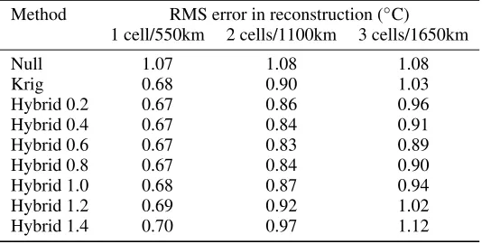
The reconstructions are compared numerically in Table
1, which shows the RMS difference between the original
and reconstructed maps averaged over all the months in
the temperature series. Results are given for the null and
kriging reconstructions, and for the hybrid calculation with
s varying from 0.2 to 1.4. Best results are obtained for
s≈0.6, representing a compromise between the improving
land reconstruction and deteriorating SST reconstruction.
The value of the RMS difference is bounded by the noise
level in the grid values.
Of more interest in this work are the accuracy of the
global temperature reconstructions. The previous results
do not directly address this question because the regions
of the globe affected by poor coverage are not uniformly
regions, an estimate must be made on the basis of the
error in reconstructing temperatures at the boundaries of the
unobserved regions.
Three test cases are therefore constructed by further
reducing the coverage of the HadCRUT4 data at the edges
of the unobserved regions. A mask is applied to remove the
values from cells whose centres are within 600, 1150 or
1700km of a cell with no observations. The masked cells
will be reconstructed by the three methods used earlier, and
the reconstructed values compared to the observations. The
coverage of the original and reduced coverage datasets is
illustrated in Figure 5. The 600km dataset involves omitting
an additional 16% of the globe from the observed data,
comparable to the 18% already missing from that data.
Two tests are used for comparing the results:
1. A difference map is calculated between the original
and reconstructed temperatures for the masked cells.
The mean and RMS of this map give a measure
of the bias and error in reconstructing cells in the
geographical regions of interest over a range of
distances from the nearest observation.
2. The differences for the masked cells are extrapolated
into the regions of the map where no observations
are available, using inverse distance interpolation
(weighted by distance−4). All cells for which
observations are available are then set to zero. This
gives an estimate of how the global mean temperature
estimate would be biased if the unobserved cells
were reconstructed with the same error as the closest
available reconstructed cells.
For each test the bias (measured by the area weighted
mean of the difference between the original and
recon-structed values), and the error (measured by the area
weighted RMS difference between the original and
recon-structed values) are presented for the period from 2005 on
when bias is expected to be critical.
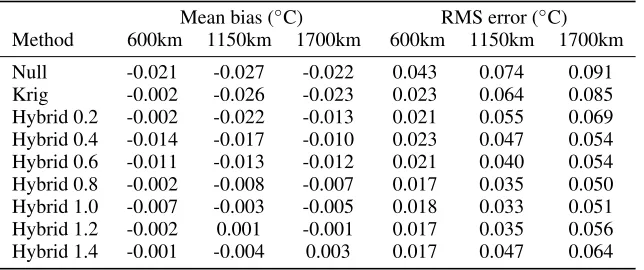
The results of reconstructing the omitted cells are shown
in Table (2). Kriging gives a lower RMS error over the
masked region than the null reconstruction in every case,
although its performance degrades as the extrapolation
range increases, and the bias is variable. The hybrid
method gives both a better mean bias and RMS error
than Kriging, and the results degrade more slowly with
increasing extrapolation range. The optimal scale factors
for the satellite data is in the range 0.8-1.2 in each case.
The month-by-month error for the 600km test using null,
kriging and hybrid (s= 1) reconstructions is shown in
Figure (6) for the years 1997-2012. The reduced error of
the kriging and hybrid reconstructions is apparent, and the
hybrid reconstruction also avoids the significant cool bias in
the other reconstructions over the period 2009-2011.
The results of projecting of the reconstructed values into
the unobserved region are shown in Table (3). This presents
a harder challenge, since the unobserved region is being
reconstructed primarily from those cells most remote from
any included observation, and the fragmentary coverage
means that the effective extrapolation range for such cells
is much larger than the quoted figure. Accordingly, for the
600km calculation kriging is only marginally better than no
reconstruction and at longer ranges it provides no benefit.
However the hybrid method shows a significant benefit at
all ranges with only limited degradation with range.
These results indicate that reconstruction of the regions
of the globe where coverage is poor is best achieved with
the hybrid method, using a scale for the satellite data in
the region of 1.0. This is in contrast with the result for the
globe in general, where optimal results are achieved by a
land and ocean, or failing that a hybrid calculation with the
satellite data down-weighted.
What is the reason for this difference? The largest
coverage holes are over Antarctica, Africa and the Arctic.
Antarctica and Africa are land, where the hybrid method
performs best. The unobserved region of the Arctic is
primarily sea ice. From the point of view of the atmosphere,
snow covered ice is similar to snow covered land.
More importantly the additional heat transfer mechanism
provided by the mixing of surface water is not present
(Barry and Chorley 2009), so there is reason to suspect that
the Arctic may behave more like land and thus be better
predicted by the hybrid method. However it is also possible
that this result arises from Arctic temperature measurements
coming primarily from land stations, e.g. Alert, Canada and
Tikhaya Bay, Russia.
3. Global reconstruction results
The kriging and hybrid methods have been applied to the
full HadCRUT4 ensemble median data to obtain global
temperature reconstructions. A global mean temperature
estimate is then calculated using an area weighted mean
of the map cells. The results are compared over the period
of the satellite data in Figure (8) using 12 and 60 month
moving averages. The kriging and hybrid reconstructions
are compared to the null reconstruction, which corresponds
to the HadCRUT4 data except in that the baseline period has
been adjusted and a global mean is calculated instead of the
Hadley practice of calculating the mean of the hemispheric
means.
The kriging and hybrid reconstructions give very
consistent results over most of the satellite era, but show
divergence from the null series over parts of the record.
Of particular interest are the periods 2005-present when
the new reconstructions show warmer temperatures than the
null series, and 1997-2000 when the new reconstructions are
cooler than the null series, with the hybrid results showing
cooler temperatures than kriging. The 60 month moving
average shows the impact of coverage, both on the 1998
peak and more significantly on recent temperatures.
How do different regions of the planet contribute to
coverage bias? The difference between the null and hybrid
reconstructions is calculated for three latitude bands. The
mean of the resulting maps provides a measure of coverage
bias due to limited coverage in each band in turn. The
results are shown in Figure (7) using 12 and 60 month
moving averages. Incomplete coverage of the rapidly
warming Arctic is the principal cause of coverage bias since
2005, despite the comparatively limited area affected. The
Antarctic shows much more variability on short time scales
owing to the larger area affected, however there is less
trend. Notable however is a large warm bias spanning the
period 1997-2000. The rest of the world (of which central
Africa is the primary region of poor coverage) contributes
comparatively little temperature bias. The 60 month smooth
gives a clearer picture of the effect of bias on longer term
trends. The sum of these contributions is comparable to the
results in Figure (1).
Trends from 1997 to the present are particularly impacted
by coverage bias (and have also been the subject of
significant media coverage, see for example The Telegraph
2013). The trends over this period have therefore been
calculated for the three series and are given in Table
(4), along with corresponding trends for the HadCRUT4,
NCDC, GISTEMP and NCEP/NCAR temperature data.
Both the kriging and hybrid series yield similar trends and
both show faster warming than GISTEMP. The difference
in trend between the original HadCRUT4 data and the null
reconstruction is apparent, and arises from the reduction in
bias due to changes in coverage over the trend period as
The NCEP/NCAR trend is higher than for the
observational records. Most of this difference comes from
mid-latitudes and from ocean rather than land data (see
supplementary information), however the high latitude
trends are in good agreement with the hybrid reconstruction.
The increased trend in the kriging reconstruction in
comparison to GISTEMP is probably related to the
additional corrections in the HadSST3 data.
The trends in the global series do not reach the 2σ
significance level primarily because inter-annual variability
due to the El Ni˜no southern oscillation (ENSO) inflates the
uncertainty. Foster and Rahmstorf (2011) find that removing
the ENSO influence and other natural influences reduces the
trend uncertainty sufficiently to make the remaining trend
statistically significant.
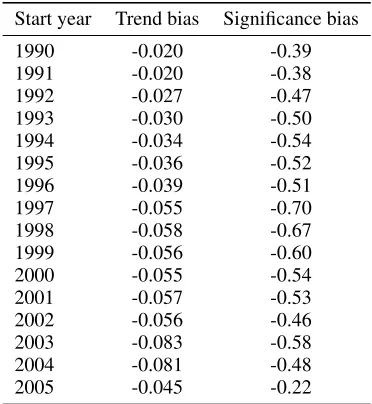
The coverage bias in the HadCRUT4 data estimated using
the hybrid data is shown in Table (5). It is notable that the
trend bias is maximised for starting dates around 1998, and
then again around 2003. Also of interest is the effect on the
statistical significance of the trend, which increases as the
number of months raised to the power 3/2. A rough estimate
of this impact may be calculated from the ratio of the bias
trend to the uncertainty in the temperature trend. By this
metric temperature trends starting in 1997 are maximally
misleading with respect to the statistical significance of the
resulting trend.
The impact of coverage bias on the 1997-2012 trend is
greatest in the winter and smallest in the summer: The
estimated bias in the trend is -0.087◦C decade−1 (DJF),
-0.049◦C decade−1 (MAM), -0.028◦C decade−1 (JJA) and
-0.055◦C decade−1(SON).
3.1. Uncertainty in the global temperature reconstruction
The uncertainty in the HadCRUT4 global temperature
reconstruction arises from a number of sources and is
discussed in detail by Morice et al. (2012). Since the
reconstructions presented here preserve the map cell values
for cells where HadCRUT4 has data, most of those
uncertainties are unaffected by this analysis.
The principal difference comes in the coverage
uncer-tainty term. Moriceet al.(2012) estimate this by reducing
the coverage of the NCEP/NCAR data to match the
Had-CRUT4 data for every available month from the reanalysis
and determining the error in the resulting global temperature
estimate. A similar approach may be applied for the kriging
method, however the hybrid method is problematic in that
it is dependent on the satellite temperature observations,
which in turn contribute to the reanalysis data.
Currently the best available estimate of the coverage
uncertainty is therefore that obtained in the validation tests
in section 2.4, and presented in tables (2) and (3). The
600km coverage reduced data leaves an additional area
of the globe unobserved which is comparable to the area
uncovered in the HadCRUT4 data, however extrapolation to
a radius of 1200km is required to achieve global coverage.
On this basis the uncertainty due to coverage bias is
estimated at between 0.028 and 0.049◦C for the kriging
results and between 0.018 and 0.033◦C for the hybrid
results. These values must be combined with the other
uncertainties as outlined by Moriceet al.(2012).
4. Discussion
This study raises the following issues:
1. Global temperature reconstructions from diverse
sources all suggest significant coverage bias in the
HadCRUT4 record over the past decades or two.
2. A method for producing a global temperature
reconstruction from incomplete data must pass
rigorous validation tests. Several such tests are
proposed.
3. A hybrid reconstruction using satellite data as a
and outperforms conventional extrapolation for the
regions of interest.
4. The impact of coverage on recent temperature trends
leads to trends starting around 1997 being particularly
misleading.
The Arctic has experienced a very rapid temperature
change over recent years through some combination of
polar amplification of greenhouse warming, albedo change
due to both black carbon and snow/ice loss and possibly
some contribution of multidecadal variability (AMAP 2011;
Semenov et al. 2010). The pace of this change means
that Arctic coverage has dominated bias in the global
temperature estimates, despite the unobserved region being
rather smaller than in the Antarctic. On this basis the
problem of coverage bias may exist whenever the Arctic
has experienced rapid warming (or cooling) in the past.
However, given the magnitude of recent Arctic warming and
polar amplification relative to global trends, it is expected
those previous periods of warming (or cooling) in the Arctic
are unlikely to bias the record to a greater extent than the
bias recorded in recent decades by this study.
The main benefit of the hybrid method is to bring
observational data to bear on the question of coverage
bias. However the method is dependent on the satellite
data and so only applicable from 1979. Given that the
hybrid results are not very different from the kriging
results, simple extrapolation appears to be justified for
current levels of global coverage. In practice the choice
of extrapolation method makes little difference once the
Antarctic stations are available: Kriging, the GISTEMP
kernel smoothing method, inverse distance weighting and
even basic nearest neighbour give very similar results,
especially used in combination with a 1200km cutoff as
employed by GISTEMP (see supplementary information).
For periods prior to the establishment of the Antarctic
stations when coverage is less complete, coverage bias
remain an issue.
The impact of coverage bias on trends starting around
1997-1998 is particularly unfortunate, given that the strong
El Nino event of 1997-1998 (and a string of La Nina
events over recent years) has also impacted trends over
the same period (Foster and Rahmstorf 2011). As a result,
the widespread reporting of HadCRUT4 temperature trends
starting in 1997 or 1998 is doubly misleading with respect
to the underlying temperature trend.
The NCDC temperature series has similar coverage
issues around the poles to the HadCRUT4 data, although
coverage at low latitudes is better. The mean coverage above
60N since 1979 is 63% for the NCDC data compared to 65%
for HadCRUT4. Since most of the bias comes from higher
latitudes, recent trends in the NCDC data are expected to be
similarly impacted to the HadCRUT4 trends.
A station-by-station investigation of the skill of the
reconstruction methods across the Arctic and Antarctic
would be of interest in further characterizing the behaviour
of the two reconstruction methods described here. The
possibility of separate methods or satellite scale factors
for land and ocean data is interesting, although it raises
the issue of whether sea ice should be treated as land or
ocean. It is hoped that the preliminary global temperature
reconstructions presented here, by highlighting the potential
scale of the bias in the short-term temperature trends,
will provide an impetus for other groups to look at the
problem using more sophisticated tools such as climate and
reanalysis models.
Data and methods for this paper are available at
http://www-users.york.ac.uk/˜kdc3/
Acknowledgements
This work was produced without funding in the authors’
own time, however KC is grateful to the University of
York for providing web space for distribution of the data
and methods. The authors would also like to acknowledge
the online community of professional and amateur climate
scientists who have provided helpful comments and advice
over the 18 months of the work, and in particular John
Kennedy at the Hadley Centre who provided useful
feedback on some very rudimentary initial results.
References
AMAP. 2011. Snow, water, ice and permafrost in the arctic (swipa).Oslo:
Arctic Monitoring and Assessment Programme (AMAP)..
Barry R, Chorley R. 2009.Atmosphere, weather & climate. Routledge.
Cressie N. 1990. The origins of kriging.Mathematical Geology22(3):
239–252.
Daily Mail. 2012. Global warming stopped 16 years ago, reveals met
office report quietly released... and here is the chart to prove it. URL
http://www.dailymail.co.uk/sciencetech/article-
2217286/Global-warming-stopped-16-years-ago-
reveals-Met-Office-report-quietly-released--chart-prove-it.html. Retrieved: 2013-03-12.
Folland C, Parker D. 1995. Correction of instrumental biases in
historical sea surface temperature data.Quarterly Journal of the Royal
Meteorological Society121(522): 319–367.
Foster G, Rahmstorf S. 2011. Global temperature evolution 1979–2010.
Environmental Research Letters6(4): 044 022.
Global Warming Policy Foundation. 2012. No underlying global
warming in recent years. URL
http://www.thegwpf.org/no-underlying-global-warming-in-recent-years/.
Retrieved: 2013-03-12.
Hansen J, Ruedy R, Sato M, Lo K. 2010. Global surface temperature
change.Reviews of Geophysics48(4): RG4004.
Hansen J, Sato M, Ruedy R, Lo K, Lea DW, Medina-Elizade M. 2006.
Global temperature change.Proceedings of the National Academy of
Sciences103(39): 14 288–14 293.
Hausfather Z, Menne MJ, Williams CN, Masters T, Broberg R, Jones
D. 2013. Quantifying the effect of urbanization on us historical
climatology network temperature records. Journal of Geophysical
Research: Atmospheres.
Kalnay E, Kanamitsu M, Kistler R, Collins W, Deaven D, Gandin L,
Iredell M, Saha S, White G, Woollen J,et al.1996. The ncep/ncar
40-year reanalysis project.Bulletin of the American meteorological Society
77(3): 437–471.
Karl TR, Williams Jr CN, Young PJ, Wendland WM. 1986. A model to
estimate the time of observation bias associated with monthly mean
maximum, minimum and mean temperatures for the united states.
Journal of Climate and Applied Meteorology25(2): 145–160. Kaufmann RK, Kauppi H, Mann ML, Stock JH. 2011. Reconciling
anthropogenic climate change with observed temperature 1998–2008.
Proceedings of the National Academy of Sciences108(29): 11 790– 11 793.
Kennedy J, Rayner N, Smith R, Parker D, Saunby M. 2011. Reassessing
biases and other uncertainties in sea surface temperature observations
measured in situ since 1850: 2. biases and homogenization.Journal of
Geophysical Research116(D14): D14 104.
Mears CA, Schabel MC, Wentz FJ. 2003. A reanalysis of the msu channel
2 tropospheric temperature record.Journal of Climate16(22): 3650– 3664.
Mears CA, Wentz FJ. 2009. Construction of the remote sensing systems v3.
2 atmospheric temperature records from the msu and amsu microwave
sounders. Journal of Atmospheric and Oceanic Technology 26(6):
1040–1056.
Meehl GA, Arblaster JM, Fasullo JT, Hu A, Trenberth KE. 2011.
Model-based evidence of deep-ocean heat uptake during surface-temperature
hiatus periods.Nature Climate Change1(7): 360–364.
Met Office. 2009. New evidence confirms land warming record.
URL http://www.metoffice.gov.uk/news/releases/
archive/2009/land-warming-record. Retrieved:
2013-03-01.
Morice CP, Kennedy JJ, Rayner NA, Jones PD. 2012. Quantifying
uncertainties in global and regional temperature change using an
ensemble of observational estimates: The hadcrut4 data set.Journal of
Geophysical Research117(D8): D08 101.
Muller RA, Rohde R, Jacobsen R, Muller E, Perlmutter S, Rosenfeld A,
Wurtele J, Groom D, Wickham C. 2012. A new estimate of the average
earth surface land temperature spanning 1753 to 2011.Geoinformatics
& Geostatistics: An Overview.
Peterson TC, Vose RS. 1997. An overview of the global historical
climatology network temperature database.Bulletin of the American
Meteorological Society78(12): 2837–2850.
Rohde R. 2013. Comparison of berkeley earth, nasa giss, and hadley
cru averaging techniques on ideal synthetic data. URL http:
Retrieved: 2013-03-01.
Semenov VA, Latif M, Dommenget D, Keenlyside NS, Strehz A, Martin
T, Park W. 2010. The impact of north atlantic-arctic multidecadal
variability on northern hemisphere surface air temperature.Journal of
Climate23(21): 5668–5677.
Smith TM, Reynolds RW, Peterson TC, Lawrimore J. 2008. Improvements
to noaa’s historical merged land-ocean surface temperature analysis
(1880-2006).Journal of Climate21(10): 2283–2296.
Spencer RW. 1990. Precise monitoring of global temperature trends.
Science247: 1558–1558.
Stokes N. 2011. Cell weighting schemes for the earth. URL http:
//moyhu.blogspot.pt/2011/08/cell-weighting-schemes-for-earth.html. Retrieved: 2013-03-01.
The Telegraph. 2013. Look at the graph to see the evidence of
global warming. URL http://www.telegraph.co.uk/
earth/environment/globalwarming/9919121/Look-
at-the-graph-to-see-the-evidence-of-global-warming.html. Retrieved: 2013-03-12.
Thompson DW, Kennedy JJ, Wallace JM, Jones PD. 2008. A large
discontinuity in the mid-twentieth century in observed global-mean
surface temperature.Nature453(7195): 646–649.
Williams CN, Menne MJ, Thorne PW. 2012. Benchmarking the
performance of pairwise homogenization of surface temperatures in the
united states.Journal of Geophysical Research117(D5): D05 116.
A. Ordinary Kriging
Ordinary kriging is applied to reconstruct a field for which
the covariance function as a function of distance is known,
but the mean of the field is unknown. Values of the field at
a coordinate~xare estimated using a linear combination of
the observed values at coordinates~xi, i= 1...N. For a field
T:
T(~x) = N
X
i=1
λi(~x)T(~xi) (2)
λi is the weight given to the observation at coordinate~xi.
The weights are determined to minimize the variance of the
estimate at each position, and are determined from the by
solving the following matrix equation:
λ1(~x)
... λN(~x)
µ =
C(~x1, ~x1) ... C(~x1, ~xN) 1
... ... ... ... C(~xN, ~x1) ... C(~xN, ~xN) 1
1 ... 1 0
−1
C(~x, ~x1)
... C(~x, ~xN)
1 (3)
C(~x, ~y) is the covariance of observations located at
coordinates~x, ~y. It is usually approximated as a function
of the distance between~xand~y, which is in turn calculated
using the available observations.
The use of kriging with gridded rather than station data
limits the number of observations available, so a
parsi-monious parameterisation is adopted. A single exponential
term provides a reasonable fit to the semivariogram, using a
function of the following form.
C(~x, ~y) =αexp(−(|~x−~y|)/d) (4)
α and d are the parameters of the covariance function.
For the purposes of this work,αis irrelevant, however d
provides a scale length for the extrapolation function in
kilometres.
dis determined from the semivariogram of the observed
every pair of observed temperatures in every month of the
data and averaging the results in 300km radial bins.The
resulting values are subtracted from the RMS difference for
cells more than 5000km apart to give a covariance estimate.
The analytic approximationCis fitted to this data. For the
HadCRUT4 datadhas a value of approximately 830km, and
for the hybrid data 680km.
Muller et al. (2012) calculate inter-station correlations
directly instead of using the variogram, and use the
correlations instead of covariances. This approach was
tested with the gridded data and gave rise to values of d
about 25% larger than the variogram method, however the
Table 1. RMS difference between original and reconstructed cell temperatures calculated over all observed cells when omitting one or more rows of data and reconstructing the central row from rows separated by the specified distance.
Method RMS error in reconstruction (◦C) 1 cell/550km 2 cells/1100km 3 cells/1650km
Null 1.07 1.08 1.08
Krig 0.68 0.90 1.03
Hybrid 0.2 0.67 0.86 0.96
Hybrid 0.4 0.67 0.84 0.91
Hybrid 0.6 0.67 0.83 0.89
Hybrid 0.8 0.67 0.84 0.90
Hybrid 1.0 0.68 0.87 0.94
Hybrid 1.2 0.69 0.92 1.02
Table 2. Mean bias and RMS error between original and reconstructed global temperatures calculated over the omitted cells using the reconstructed values for the omitted cells. Results are for the period 2005/01-2012/12 and are given for the three reduced coverage maps described in Figure (5).
Mean bias (◦C) RMS error (◦C)
Method 600km 1150km 1700km 600km 1150km 1700km
Null -0.021 -0.027 -0.022 0.043 0.074 0.091
Krig -0.002 -0.026 -0.023 0.023 0.064 0.085
Hybrid 0.2 -0.002 -0.022 -0.013 0.021 0.055 0.069
Hybrid 0.4 -0.014 -0.017 -0.010 0.023 0.047 0.054
Hybrid 0.6 -0.011 -0.013 -0.012 0.021 0.040 0.054
Hybrid 0.8 -0.002 -0.008 -0.007 0.017 0.035 0.050
Hybrid 1.0 -0.007 -0.003 -0.005 0.018 0.033 0.051
Hybrid 1.2 -0.002 0.001 -0.001 0.017 0.035 0.056
Table 3. Mean bias and RMS error between original and reconstructed global temperatures calculated over theunobserved cellsby extrapolat-ing the reconstructed values for the omitted cells into the unobserved region. Results are for the period 2005/01-2012/12 and are given for the three reduced coverage maps described in Figure (5).
Mean bias (◦C) RMS error (◦C)
Method 600km 1150km 1700km 600km 1150km 1700km
Null -0.032 -0.033 -0.032 0.070 0.071 0.071
Krig -0.033 -0.033 -0.032 0.068 0.073 0.073
Hybrid 0.2 -0.005 -0.028 -0.028 0.055 0.063 0.063
Hybrid 0.4 -0.026 -0.024 -0.008 0.052 0.055 0.051
Hybrid 0.6 -0.022 -0.019 -0.019 0.046 0.049 0.048
Hybrid 0.8 -0.019 -0.015 -0.009 0.042 0.045 0.043
Hybrid 1.0 -0.016 -0.004 -0.010 0.042 0.043 0.044
Hybrid 1.2 -0.007 -0.006 -0.006 0.041 0.047 0.047
Table 4. Temperature trend in◦C decade−1in the GISTEMP, NOAA
and HadCRUT4 temperature series and in the null, kriging and hybrid reconstructions. The standard error in the trend is calculated according to the method of Foster and Rahmstorf (2011) assuming an ARMA(1,1) error model.
Dataset Trend±σ
NCEP/NCAR 0.178±0.107 GISTEMP 0.080±0.067
NOAA 0.043±0.062
Table 5. Bias in HadCRUT4 temperature trends running from various dates to the present, estimated using the hybrid data (s= 1.0), in units of◦C decade−1. The impact of the bias on the significance of the trend
is given in the third column.
Start year Trend bias Significance bias
1990 -0.020 -0.39
1991 -0.020 -0.38
1992 -0.027 -0.47
1993 -0.030 -0.50
1994 -0.034 -0.54
1995 -0.036 -0.52
1996 -0.039 -0.51
1997 -0.055 -0.70
1998 -0.058 -0.67
1999 -0.056 -0.60
2000 -0.055 -0.54
2001 -0.057 -0.53
2002 -0.056 -0.46
2003 -0.083 -0.58
2004 -0.081 -0.48
HadCRUT4 land/ocean
GISTEMP land/ocean
UAH satellite
NCEP/NCAR reanalysis
Figure 1. Temperature trends for the 16 year period 1997/1-2012/12
in◦C decade−1 for HadCRUT4 and three near global reconstructions:
Null reconstruction
Range = 1 cell/550km
Kriging Hybrid
Range = 2 cells/1100km
Kriging Hybrid
Range = 3 cells/1650km
Kriging Hybrid
Figure 4. RMS difference in◦C between observed temperatures and 36-fold cross validated reconstruction, omitting different numbers of latitude bands
Figure 6. Error in the reconstruction of the mean temperature of the observed region of the HadCRUT4 data using only data from a map whose coverage has been reduced by 600km around every unobserved grid cell.
Error in◦C are shown by month on the period 1997/01-2012/12 for the
a)
b)
Figure 7. Coverage bias in the HadCRUT4 global mean (rather than mean of the hemispheric means) estimated using the hybrid (s= 1.0)
a)
b)