This is a repository copy of
Modelling for Robust Feedback Control of Fluid Flows
.
White Rose Research Online URL for this paper:
http://eprints.whiterose.ac.uk/84870/
Version: Accepted Version
Article:
Jones, B., Heins, P.H., Kerrigan, E.C. et al. (2 more authors) (2015) Modelling for Robust
Feedback Control of Fluid Flows. Journal of Fluid Mechanics, 769. 687 - 722 . ISSN
1469-7645
https://doi.org/10.1017/jfm.2015.84
[email protected] https://eprints.whiterose.ac.uk/ Reuse
Unless indicated otherwise, fulltext items are protected by copyright with all rights reserved. The copyright exception in section 29 of the Copyright, Designs and Patents Act 1988 allows the making of a single copy solely for the purpose of non-commercial research or private study within the limits of fair dealing. The publisher or other rights-holder may allow further reproduction and re-use of this version - refer to the White Rose Research Online record for this item. Where records identify the publisher as the copyright holder, users can verify any specific terms of use on the publisher’s website.
Takedown
If you consider content in White Rose Research Online to be in breach of UK law, please notify us by
J. F. M O R R I S O N
A N DA. S. S H A R M A
1Department of Automatic Control and Systems Engineering, University of Sheffield, Sheffield, S1 3JD, UK
2Department of Electrical and Electronic Engineering, Imperial College London, SW7 2AZ, UK
3 Department of Aeronautics, Imperial College London, London, SW7 2AZ, UK 4 Engineering and the Environment, University of Southampton, Highfield, Southampton,
SO17 1BJ, UK
(Received ?; revised ?; accepted ?. - To be entered by editorial office)
This paper addresses the problem of designing low-order and linear robust feedback controllers that provide a priori guarantees with respect to stability and performance when applied to a fluid flow. This is challenging since whilst many flows are governed by a set of nonlinear, partial differential-algebraic equations (the Navier-Stokes equations), the majority of established control system design assumes models of much greater simplicity, in that they are firstly: linear, secondly: described by ordinary differential equations, and thirdly: finite-dimensional. With this in mind, we present a set of techniques that enables the disparity between such models and the underlying flow system to be quantified in a fashion that informs the subsequent design of feedback flow controllers, specifically those based on theH∞ loop-shaping approach. Highlights include the application of a model refinement technique as a means of obtaining low-order models with an associated bound that quantifies the closed-loop degradation incurred by using such finite-dimensional approximations of the underlying flow. In addition, we demonstrate how the influence of the nonlinearity of the flow can be attenuated by a linear feedback controller that employs high loop gain over a select frequency range, and offer an explanation for this in terms of Landahl’s theory of sheared turbulence. To illustrate the application of these techniques, a H∞ loop-shaping controller is designed and applied to the problem of reducing perturbation wall-shear stress in plane channel flow. DNS results demonstrate robust attenuation of the perturbation shear-stresses across a wide range of Reynolds numbers with a single, linear controller.
Key words:
1. Introduction
The ability to exert control over fluid flows has received renewed attention in recent years, with the potential to improve the efficiency of fluid-based systems thereby of-fering wide-ranging economic and environmental benefits across a range of industries. Examples include the lowering of fuel costs and greenhouse gas emissions via the drag reduction of aircraft (Bushnell 2003) and shipping (Corbett & Koehler 2003), optimal
mixing of chemical reagents (Couchman & Kerrigan 2010) and wind turbine gust alle-viation (Frederick et al. 2010), with many more examples stemming from the natural world (Fish & Lauder 2006). Attempts to control fluid flow are typically classified into three broad categories (Gad-el-Hak 2000): passive (e.g. Choiet al.(1993)), active open-loop (e.g. Sturzebecher & Nitsche (2003); Hanson et al. (2010)) and active closed-loop control (e.g. Bewley (2001); Hogberg et al.(2003); Kim (2003); Kim & Bewley (2007); Semeraroet al. (2011)), each with their own merits and extensively discussed in many review papers and textbooks (e.g. Bewley (2001); Colliset al.(2004); Gad-el-Hak (2000)). This paper is concerned with the use of active (in the sense that powered actuators are assumed) closed-loop control of fluid flows. There are compelling reasons for employing such control, despite it being the most difficult to implement practically, owing to the dual requirements of sensing and actuation. Principal amongst these reasons is the unique ability of feedback controllers to reject the effects ofuncertaintyupon the desired outputs of a system (Vinnicombe 2001), a concept that is of central importance in obtaining suitable control models for fluid flows, and which is the primary focus of this paper.
Uncertainties arise not only from the intrinsic model assumptions but also from exoge-nous disturbances inherent to practical problems. To synthesise a feedback controller for a fluid flow, a model describing the dynamics of the system is required, where the system (or “plant”) comprises actuators, sensors and the flow itself, in addition to the spatial interconnections between these subsystems. The dynamics of electromechanical compo-nents, such as pressure sensors (Arthur et al.2006) and synthetic jet actuators (Gallas
et al. 2003), are typically well approximated by lumped-parameter models consisting of a few ordinary differential equations (ODEs). However, this is seldom the case for fluid flows, described in many cases by the incompressible Navier-Stokes equations:
∂V(x, t)
∂t =−V(x, t)· ∇V(x, t)− ∇P(x, t) + 1
Re∇
2
V(x, t) +g(x, t), (1.1a)
0 =∇ ·V(x, t), (1.1b)
where V(x, t) and P(x, t) are the velocity and pressure fields, respectively, evolving in domain Ω∈R3under the influence of an external forcingg(x, t), withx∈Ω andt∈R+. Boundary and initial conditions are given as:
V(x, t) =V∂(x, t) withx∈∂Ω, V(x,0) =V0,
where ∂Ω is the boundary of the domain. In contrast to (1.1), the majority of existing modern control systems theory relies upon models in standard, linearstate-spaceform:
˙
x(t) =Ax(t) +Bu(t), (1.2a)
y(t) =Cx(t) +Du(t), (1.2b)
where A∈Rn×n,B ∈Rn×m, C ∈Rq×n, D∈Rq×m,x(t)∈Rn is the state vector with
initial state x(0) =x0, u(t)∈ Rm is the vector of control inputs and y(t) ∈ Rq is the
measurement vector. The states in (1.2a) evolve according to a finite-dimensional set of linear ODEs, and for the purposes of practical controller implementation it is desirable that the number of states be small, typically no more thann∼ O(102). This means that
in order to apply standard controller synthesis algorithms, the control model (1.2) must be of much greater simplicity than the underlying flow model (1.1).
a priori guarantees concerning the degree of stability of the closed-loop system, subject to model uncertainty and exogenous disturbances. The starting point for generating such controllers is a model of the form (1.2) that describes the linear dynamics of the flow.
1.1. The importance of linear dynamics
A question that naturally arises is under what circumstances can a linear feedback con-troller, synthesised from a linear model (1.2), actually stabilise a flow governed by (1.1)? Although linearisations of (1.1) are inevitably unable to capture the nonlinear dynam-ics that endow turbulent flows with their ‘multiscale’ characteristdynam-ics (Kim & Bewley 2007), they are widely accepted as being relevant in explaining such phenomena as tran-sition to turbulence in wall-bounded flows (Semeraroet al. 2011; Butler & Farrell 1992; Trefethenet al.1993; Schmid & Henningson 2000), as well as at least some of the mech-anisms that sustain turbulence in such flows. In this respect, linear effects have received some attention since Batchelor and Proudman’s seminal work on rapid distortion the-ory (RDT) (Hunt & Carruthers 1990; Lee et al.1990). Farrell & Ioannou (1993, 1996) have suggested that the linearised Navier-Stokes equations in plane channel flow un-der stochastic forcing can exhibit behaviour reminiscent of the streamwise vortices and streaks characteristic of turbulent flow. Transient growth studies have highlighted the im-portance of the linear operator to streak formation (Butler & Farrell 1992; Chernyshenko & Baig 2005). The input-output (gain-based) analysis by Jovanovic & Bamieh (2005) of the linearised Navier-Stokes equations also revealed the importance of long streaky structures. Kim & Lim (2000) demonstrated in simulations of turbulent channel flow that the turbulence decays without the term coupling the wall-normal vorticity and the wall-normal velocity in the linearised Navier-Stokes equations.
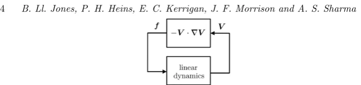
fluctua-Figure 1.System-level description of the turbulence process. The nonlinearity produces a forcef :=−V · ∇V that acts as a disturbance input to the linear subsystem.
tions is linear and underpins the generation of turbulent fluctuations, the linear control strategy is effective. Shear interaction is a linear RDT approximation embodied in the Orr-Sommerfeld-Squire (OSS) equations: it is governed by the wall-normal disturbance velocity which appears in the coupling term and which is related to the pressure via the linear ‘fast’ source term in the Poisson equation for pressure fluctuations (Kim 1989; Dunn & Morrison 2003). As a result, the response to forcing of the wall-normal velocity and pressure is rather quicker than that of both the streamwise or spanwise velocities. This occurs because the shear interaction timescale is considerably shorter than either the viscous or turbulence timescales (Landahl 1977) so that the Reynolds stresses are less effective. Batchelor & Townsend (1956) have shown that pressure-gradient fluctua-tions drive the momentum field, appearing as spikes in the instantaneous mean-square acceleration. Sharmaet al.(2011) have also shown that first, these fluctuations reach a maximum at y+
≈20, and second, the forcing is at a maximum at the same location. This explains why the linear controller is effective even though it is operating on the wall-normal component alone. Landahl’s theory (Landahl 1975, 1967) also provides a ‘wave-guide’ model of the viscous sublayer in which the least dispersive components are those of the wall-normal velocity component and pressure fields. Clearly, understand-ing these linear mechanisms and the extent to which they are local to the wall has a significant bearing on potential drag-reduction strategies: for active, linear control, a fundamental appreciation of the shear-interaction timescale is a prerequisite and clearly, pressure is a key component to the interaction between the inner, wall region and the outer layer (Townsend 1961; Bradshaw 1967; Morrison 2007).
Given the importance of suppressing turbulence for reducing skin-friction drag, much attention has been focussed on designing controllers for wall-bounded flows, particularly plane channel-flows (Bewley & Liu 1998; Leeet al.2001; Hogberget al. 2003; Baramov
et al. 2004; Hoepffneret al. 2005; Kim & Bewley 2007). Kim (2003) examined different types of Linear Quadratic Regulator (LQR), also for turbulent channel flow, to minimise (1) wall-shear stress fluctuations, (2) turbulent kinetic energy, and (3), the linear coupling term. All resulted in significant drag reduction, a common feature being a weakening of quasi-streamwise vortices resulting in reduced high skin-friction extrema at the wall. There are many models of the near-wall cycle (see, for example, Hamiltonet al.(2006)) but all suggest that transient energy growth, as described by the OSS equations, provides a linear paradigm of near-wall turbulence (Butler & Farrell 1992). Central to our approach is that, for a model-based feedback controller to be successful, the role of linear dynamics can be exploited. A key challenge is that much of our knowledge derives from direct numerical simulations at low Reynolds number (Robinson 1991) and, as a result, our understanding is primarily kinematic. Here the approach is dynamic, in the sense that any form of control implies the selective response of a flow to forcing.
[image:5.595.96.462.102.188.2]mech-from model uncertainty and the nonlinear forcing of the flow, respectively.
anisms play in the transition process (Pringle & Kerswell 2010; Pringle et al. 2012; Cherubini et al. 2010, 2011) wherein the optimal perturbations differ considerably in terms of structure and energy growth, compared to their linear counterparts.
1.2. Robust control and uncertainty in fluid flows
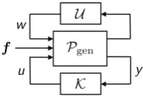
With respect to the preceding discussion, linear approximation of the flow dynamics represents just one source of uncertainty between the actual flow (1.1) and state-space models (1.2) employed for controller design. It is therefore important to identify and model the other sources of uncertainty, as such information can guide the controller design process. An illustrative robust control problem is shown in Figure 2, where K denotes the feedback controller,U represents model uncertainty andPgenis the nominal
(approximate) model of the ‘generalised’ plant, that is, the linearised dynamical model of the fluid flow, the sensors and actuators, as well as the interconnection structure between the plant and controller.
The generalised plant consists of individual partitions that map the control, nonlinear forcing and model uncertainty disturbance input signals,u,f andw, respectively, to the measured output signal,y, according to:
y =Pww+Pff+Pu. (1.3a)
It is worth noting that the individual partitions aretransfer functionmatrices, obtainable from a Laplace transform of a time-domain model. For example,P can be obtained from the Laplace transform of (1.2) as follows:
P =C(sI−A)−1B+D, (1.3b)
where s ∈ C and I is the identity matrix. The aim of the present work is to design a stabilising controller K, so as to make the H∞ norm k·k∞ of the closed-loop transfer functions fromw andf toy, Pyw and Pyf, respectively, both small, where:
kPywk∞:= sup w6=0
ky(t)k2
kw(t)k2, kPyfk∞:= sup
f6=0
ky(t)k2
kf(t)k2. (1.3c) Furthermore, in the interests of robustness, the controller should achieve these aims in the presence of model uncertainty U, which represents a set of norm bounded transfer function matrices that captures this class of uncertainty. Modelling the uncertainty set again represents a trade-off between complexity and achievable performance, since U
should be general enough so that the actual plant lies within the set of all perturbed plants defined by the interconnection of U with the nominal model Pgen, but not so
[image:6.595.235.339.119.189.2]sources of uncertainty are summarised as follows:
• Model uncertainty. This takes two forms. The first of these is parametric uncer-tainty that arises owing to a lack of precise knowledge of the parameters (e.g. Reynolds number) of the system. Also, if the governing equations are linearised around an equi-librium flow solution, then the theoretical and actual mean flows may differ. Another source of parametric error might arise from numerical errors incurred during the process of eliminating the algebraic constraint (1.1b) to obtain an unconstrained system (1.2a). This arises, for example, when inverting an ill-conditioned discretised Laplacian to ob-tain the Orr-Sommerfeld matrix. Secondly, dynamic uncertainty, which is inherent in any finite-dimensional approximation of an infinite-dimensional system. Spatial discreti-sations of (1.1) only resolve a finite number of dynamic modes, typically those of low-est spatial frequency, and consequently neglect all higher frequency modes. Of those modes that are retained by a spatial discretisation, some will be better resolved than others (Boyd 2001). The problem of determining a suitable level of spatial refinement (and hence which modes are of dynamical importance) is of fundamental importance in designing controllers that can tolerate the uncertainty arising from the use of a finite-dimensional flow model. Addressing this issue is an important contribution of this paper.
• Disturbance uncertainty.In practice, a flow will be subjected to disturbances arising from a number of sources, such as uncertain boundary conditions, forcing from acoustic noise and the coupling of sensor noise into the flow via a feedback controller. Such dis-turbances may be impractical to model in any great detail, other than perhaps knowing a bound on their magnitude and the point at which they enter the closed-loop system. In addition, and as discussed in Section 1.1, the nonlinearity of the Navier-Stokes equations can be treated as an uncertain disturbance forcing acting upon the linear system. From a control systems perspective this is important, since it enables the problem of suppressing turbulence to be formulated as a disturbance rejection problem.
In summary, in order for a feedback controller to guarantee robustness to these sources of model uncertainty, the controller design process must account for each uncertainty in some way. The manner in which this can be achieved is discussed in the following section.
1.3. Addressing sources of uncertainty
If bounds on all the uncertainties listed above are known, then each uncertainty can be ‘extracted’ from the plant model to form a structured perturbation matrixU, and this structure can then be exploited in subsequent controller designs, based on structured-singular-value synthesis algorithms (Skogestad & Postlethwaite 2005). An alternative, and simpler class of uncertainty model exists in the form of unstructured uncertainty, whereby the perturbation matrix U is ‘full’. Many different unstructured uncertainty models exist (Vinnicombe 2001), such as additive uncertainty, multiplicative input un-certainty and inverse multiplicative output uncertainty, each with their own merits in terms of representing parametric, dynamic and disturbance uncertainty. An appropriate uncertainty model for closed-loop flow control, for reasons that will be discussed below, is that of coprime factor uncertainty. Background material on this subject is presented in Appendix A, but we note, briefly, that coprime factor perturbations take the form:
Pp:=
(N +UN)(M+UM)−1 , (1.4)
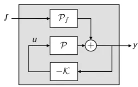
Figure 3.Feedback control diagram for disturbance rejection. The objective is to design the loop-shaping controllerKto reject the disturbance, arising form the nonlinear forcingf, upon the measured outputsy (e.g. wall shear-stress) of the flow system. The system within the shaded region is the closed-loop transfer function matrixPyf (1.5) from disturbance forcing to output. Although seemingly abstract, this class of uncertainty is particularly useful as it can be regarded as a blend of multiplicative and inverse multiplicative type uncertainties that naturally account for dynamic and parametric uncertainty, respectively (Vinnicombe 2001). It also accounts for uncertainty in the number of right-half plane system poles and zeroes, both of which impose fundamental performance limitations upon feedback controllers. It is worth emphasising that the use of such an unstructured uncertainty description greatly reduces the difficulty of modelling the uncertainty set, and hence reduces the difficulty of designing a robust controller. Indeed, in the case of coprime factor uncertainty, no effort is required at all since controller synthesis techniques that employ this description, such as theH∞ loop-shaping procedure of McFarlane & Glover (1992), automatically synthesise controllers that maximise the amount of coprime factor uncertainty that a closed-loop system can tolerate. In doing so, and as explained further in Appendix A, H∞ loop-shaping controllers also attenuate the effect of disturbances entering at different points in the system (including sensor noise). To see this is the case for rejecting the influence of the forcing arising from the nonlinearity of the flow, consider again the system described by the model (1.3a). Assuming an output feedback control law of the form u=−Ky leads to the following expression for the closed-loop transfer functionPyf that relatesf toy:
y = (I+PK)−1Pf
| {z }
Pyf
f. (1.5)
The relevant closed-loop system is depicted in Figure 3. The control objective is to re-duce the influence off upony, and this is achieved by making the gain of Pyf small (in
terms ofkPyfk∞), which in turn amounts to designing the loop-shaping controllerKto
ensure that the gain of the open-loop system PK is greater than unity, as can be seen from inspection of (1.5). Such loop-shaping controllers therefore provide a convenient framework for dealing with the parametric, dynamic and disturbance uncertainties en-countered when attempting to control flows (1.1) from controllers designed upon simpler models (1.2). This simplicity of designing robust controllers has thus meant that H∞ loop-shaping controllers have found use in a variety of applications, ranging from the flight control of vertical take-off aircraft (Hyde et al. 1995), control of combustion os-cillations (Chu et al. 2003), bluff body form-drag reduction (Dahan et al. 2012) and wind-turbine active blade-pitch control (Luet al.2014).
testing, rather than at the controller design stage. The focus of this paper, therefore, is upon obtaining state-space models (1.2) of flows described by linearisations of (1.1), that are of sufficient simplicity to enable straightforward synthesis of controllers witha priori
stability and performance guarantees.
The remainder of this paper is organised as follows. We begin in Section 2 by formulat-ing the modellformulat-ing problem. The startformulat-ing point is the linearised Navier-Stokes equations and the finishing point is a low-order, state-space model suitable for controller synthesis. On the way we show how to numerically convert a system of DAEs to one of ODEs, and the motivation for doing so. We also introduce the ν-gap metric as a useful tool from
feedback control theory and show how it can be used to efficiently derive low-order state-space models from spatial discretisations of the linearised flow system. In Section 3, aH∞ loop-shaping controller is designed from a low-order model and applied to plane channel-flow. Significant portions of this paper are expository in nature and assume little prior knowledge from the reader of feedback control, other than a rudimentary appreciation of classical loop-shaping techniques such as PID control and lead/lag compensation (˚Astr¨om & Murray 2008). To preserve clarity of exposition, some control systems material is in-cluded as appendices. In particular, background material on coprime-factor uncertainty andH∞-loop shaping is presented, as are the algorithms employed to firstly convert the semi-discretised Navier-Stokes equations into a standard state-space model.
2. Formulation of low-order control models
The dynamics of infinitesimal perturbations in a viscous, incompressible, wall-bounded flow can be described by linearisation of the Navier-Stokes equations (1.1) around a mean flow solution. Subsequent spatial discretisation yields a system in the generalised state-space (or descriptor) form:
E11 0
0 0
| {z }
ED
d dt
v(t) p(t)
| {z }
˙
xD(t)
=
A11 A12
A21 0
| {z }
AD
v(t) p(t)
| {z } xD(t)
+
B1
B2
| {z } BD
u(t), (2.1)
where v(t) ∈ Cnv and p(t)
∈ Cnp are the semi-discretised vectors of (perturbation)
velocities and pressure, respectively, and u(t) ∈ Cm is a vector of control inputs. The
state vector is xD(t), E11 ∈ Cnv×nv
is the symmetric, positive definite mass matrix and A11 ∈ Cnv×nv contains a mixture of discrete diffusion and linearised convective
terms. The matrices A12 ∈ Cnv×np and
A21 ∈ Cnp×nv represent the discrete gradient
and divergence operators, respectively, andB1∈Cnv×m and
B2 ∈Cnp×mdescribe how
the control inputs influence the states. Note that the subscript ‘D’, denotes vectors and matrices pertaining to descriptor state-space systems.
The state evolution equation (2.1), together with the measurement equation y(t) =
CDxD(t) +DDu(t), can be written as a descriptor state-space system:
EDx˙D(t) =ADxD(t) +BDu(t), (2.2a)
y(t) =CDxD(t) +DDu(t), (2.2b)
where ED, AD ∈ CnD×nD, CD ∈ Cq×nD, DD ∈ Cq×m and y(t) ∈ Cq is the vector of
measured outputs. The ordernD=nv+npof the state vector depends on the resolution,
but is typically very large for simulation models (e.g. nD > 106). For control models,
however, the number of states need not be the same, and can in fact be much lower, as discussed in more detail in Section 2.3.
Figure 4.Side view of plane channel flow and conceptual sketch of the control system. Spatially continuous actuation (transpiration) and sensing (streamwise shear stress) occurs at both walls. For a given wavenumber pair, the feedback controllerKtakes, as inputs, the sensor measure-ments ˜y, and outputs a control signal ˜u to the actuators.
two infinite, parallel, planar and stationary boundaries, as shown in Figure 4. Non-dimensionalising length scales by the channel half-height,h, velocities by the centre-line velocityUcland pressure byρUcl2, the linearised Navier-Stokes equations for
incompress-ible plane channel flow are (Aamo & Krstic 2003; McKernan 2006):
∂u ∂t =−U
∂u ∂x−v
∂U ∂y −
∂p ∂x +
1
Re∇
2u, (2.3a)
∂v ∂t =−U
∂v ∂x−
∂p ∂y +
1
Re∇
2v, (2.3b)
∂w ∂t =−U
∂w ∂x −
∂p ∂z+
1
Re∇
2w, (2.3c)
0 = ∂u ∂x +
∂v ∂y+
∂w
∂z, (2.3d)
where Re = ρUclh/µ is the Reynolds number and the mean velocity profile satisfies
U = 1−y2. In non-dimensional co-ordinates the upper and lower walls are located at
y =±1. The streamwise, wall-normal and spanwise perturbation velocitiesu, v andw, respectively, and perturbation pressurepare functions ofx,y,z andt. The initial and boundary conditions are as follows:
u(x, y, z,0) =u0, v(x, y, z,0) =v0, w(x, y, z,0) =w0, (2.4a)
u(x,±1, z, t) = 0, v(x,±1, z, t) = 0, w(x,±1, z, t) = 0. (2.4b)
For the purposes of the current investigation, it is sufficient to employ actuators and sensors that render the system (2.3) controllable and observable (˚Astr¨om & Murray 2008; Bewley & Liu 1998). Therefore, the walls are assumed continuously distributed with wall transpiration actuators and sensors capable of measuring the streamwise component of the wall-shear stress (Aamo & Krstic 2003; Bewley & Liu 1998; McKernanet al. 2006). A conceptual sketch of this arrangement is shown in Figure 4. The control objective of the present study is to attenuate the streamwise wall-shear stress perturbations. Such a control objective was employed by Lee et al. (2001) and Lim (2003), where linear controllers were synthesised that significantly reduced the wall-shear stress perturbations, leading to significant reductions in the mean drag.
can be modelled by the following inhomogenous boundary conditions on the upper and lower walls, respectively:
∂v(x,+1, z, t)
∂t :=−
1
ςv(x,+1, z, t) + 1
ςu(x,+1, z, t), (2.5a) ∂v(x,−1, z, t)
∂t :=−
1
ςv(x,−1, z, t) + 1
ςu(x,−1, z, t). (2.5b) In terms of measurements we consider the streamwise component of the wall shear stressτxy at both walls:
y(x, y, z, t) :=
τyx|y=+1
τyx|y=−1
= 1 Re ∂u ∂y + ∂v ∂x y=+1 ∂u ∂y + ∂v ∂x
y=−1
. (2.6)
Having defined inputs and outputs, the infinite-dimensional system (2.3) is then rendered finite-dimensional via spatial discretisation. The flow is Fourier-transformed in the spa-tially homogenous x and z directions, in which case the distributed control input u is approximated as follows:
u(x,±1, z, t)≈R
Nx
X
nx=1 Nz
X
nz=1
˜
u(±1, t)ei(αx+βz)
!
, (2.7)
where i := √−1, α and β are streamwise and spanwise wavenumbers, respectively, and ˜u ∈ C2 are the Fourier-transformed inputs at each wavenumber pair (α, β). The
output equation (2.6) is similarly approximated. In the inhomogenous y direction the flow is discretised on Ny Chebyshev collocation nodes (Weideman & Reddy 2000) and
the spatial y-derivatives ∂y∂ , ∂y∂22 are approximated by Chebyshev differentiation
ma-trices Ych, Ych2, respectively (Weideman & Reddy 2000). Application of the
Fourier-transform decouples the system dynamics by wavenumber, and so the flow dynamics for each individual pair (α, β) can now be expressed as a linear, finite-dimensional descriptor state-space system:
ED11 0 0 0
0 ED22 0 0
0 0 ED33 0
0 0 0 0
| {z }
ED d dt ˜ uny(t)
˜ vny(t)
˜ wny(t)
˜ pny(t)
| {z }
˙
xD(t)
=
AD11AD12 0 AD14
0 AD22 0 AD24
0 0 AD33AD34 AD41AD42AD43 0
| {z }
AD ˜ uny(t)
˜ vny(t)
˜ wny(t)
˜ pny(t)
| {z }
xD(t)
+ 0 0
BD21BD22
0 0 0 0
| {z }
BD
˜
u(t),
(2.8a)
˜
y(t) =
CD11 CD12 0 0 CD21 CD22 0 0
| {z }
CD
xD(t), (2.8b)
where ˜uny(t), ˜vny(t), ˜wny(t) and ˜pny(t) are vectors containing the Fourier transformed
velocity and pressure coefficients at theny-th collocation node (where 16ny 6Ny) for
a given wavenumber pair. The elements of the dynamics matrix are defined as:AD11 := AD22 := AD33 := −iαUny +
1
Re∆, AD12 := − dUny
dy , AD14 := −AD41 := −αI, AD24 := −AD42 := −Ych, AD34 := −AD43 := −βI, and ED11 := ED22 := ED33 := I, where i := √
−1,Uny := 1−y
2
ny and ∆ := −α
2+Y2
ch−β2 is the discrete Laplacian operator. The
control input influences the states via BD21 := [ 1 ς 0...0]
T
andBD22:=[0...0 1 ς ]
T
. In the case of streamwise shear-stress measurementsCD11 :=
1
exception of the (1,1) element ofAD22, which is set to−1/ς.
2.1. Dealing with descriptor systems: Eliminating the incompressibility constraint
Control of descriptor state-space systems (2.2) is less well understood than that for stan-dard state-space systems (1.2), and so controller synthesis becomes more straightforward if the former can be converted into the latter. This is trivial when the inverse ofED
ex-ists, since both sides of (2.2a) can be premultiplied byED−1. However, this is not possible in (2.1) sinceED is singular, owing to the assumption of incompressibility. To overcome
this difficulty, the system (2.3) is usually reformulated so that the resultingEDmatrix is
non-singular and can be inverted to yield a standard state-space system. For the case of plane channel flow, it is possible to analytically eliminate the divergence constraint (2.3d) by reformulating the system in terms of a divergence-free basis described in terms of wall-normal velocities and wall-wall-normal vorticities. A non-singularEDcan then be obtained by
using a set of basis functions that individually satisfy the boundary conditions, yielding the familiar OSS system (Schmid & Henningson 2000; Kim & Lim 2000):
d dt
˜ vny(t)
˜ ζny(t)
=
LOS 0
LC LS
| {z }
AOSS
˜ vny(t)
˜ ζny(t)
, (2.9a)
where ˜ζny(t) is the vector of Fourier transformed wall-normal vorticities at a particular
wavenumber pair. The OSS matrixAOSSconsists of the Orr-Sommerfeld matrixLOS, the
Coupling matrixLC and the Squire matrixLS:
LOS:= ∆−1
−iαUny∆ +iα d2U
ny dy2 +
1
Re∆
2
, (2.9b)
LC:=−iβ
dUny
dy , (2.9c)
LS:=−iαUny+
1
Re∆, (2.9d)
Although this reformulation has proven itself invaluable for hydrodynamic stability analyses, its use for control system design is not without limitation. For instance, it is difficult to analytically obtain divergence-free bases for more complicated flows, such as those with variable fluid properties, or those with complex geometries (Ferziger & Peri´c 1997). This is one of the main reasons why the majority of feedback flows control studies have concentrated on channel flows or similar, parallel, shear flows. Also, satisfying boundary conditions in a divergence-free basis is considerably more difficult than in the original primitive-variable basis, particularly for complex geometries. The boundary conditions, naturally expressed in terms of primitive variables, must be transformed to equivalent conditions in a divergence-free basis that is subject to higher-order spatial derivatives (e.g. fourth-order in (2.9b)). Failure to satisfy these conditions precisely results in an unphysical system, contaminated by ‘spurious’ eigenmodes (Bewley & Liu 1998).
variable form) before converting the resulting finite-dimensional descriptor system (2.2) into standard state-space form (1.2). Furthermore, this final step of projecting from descriptor to standard state space form can be performed efficiently via a numerical method (Sch¨on et al. 2003; Gerdin 2006; Shahzad et al. 2011). This is summarised in Appendix B, and has been applied successfully to the problem of flow field estimation in a non-parallel boundary layer (Joneset al.2011). From a high-level perspective, the algorithm takes, as inputs, the matrices of the descriptor system (ED,AD,BD,CD,DD),
and outputs the matrices of an equivalent (in the sense that the input-output response is identical) standard state-space system (A,B,C,D), together with a transformation matrix that relates the states xD of the former, to those of the latter x. Applying this
algorithm to the system (2.8) thus yields a standard state-space system of the form (1.2):
˙
x(t) =Ax(t) +B˜u(t), (2.10a) ˜
y(t) =Cx(t) +Du˜(t). (2.10b)
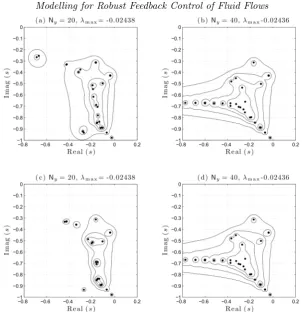
The accuracy of this projection technique can be assessed via a comparison of the spectra and pseudospectra (Trefethen & Embree 2005) ofAOSS in (2.9a), with those of
the equivalent operator Ain (2.10a). Computing the pseudospectra ofAOSS in (2.9a) is
complicated by the fact that the kinetic energy of the perturbations is naturally defined in terms of the streamwise, wall-normal and spanwise velocities, thus requiring the energy to be redefined in terms of wall-normal velocity and vorticity (see Butler & Farrell (1992) for details). The eigenvalues and ǫ-pseudospectra of AOSS and A, for the case Re =
1000, α = β = 1, are shown in Figure 5 and begin to show increasing convergence as wall-normal resolution is increased, implying that both operators exhibit the same open-loop transient and asymptotic behaviour. However, an important question to ask is whether or not such reproduction of the open-loop dynamics really matters? Specifically, to what extent does a model employed forclosed-loopcontrol need to accurately capture the open-loop dynamics of the actual flow? This issue is discussed in the following section.
2.2. Modelling for feedback control and theν-gap metric
As noted by Kim & Bewley (2007), a model that is good enough for the purpose of designing a feedback controller, need not necessarily be a good simulation model. How-ever, the converse is also true, in that a good simulation model is not always a suitable model for feedback control design (see e.g. ˚Astr¨om & Murray (2008)). It may therefore be misleading to compare the open-loop responses of systems if the objective is to design a feedback controller. This is relevant since most approaches to obtaining low-order models are based on open-loop model-reduction techniques such as balanced truncation (Zhou
et al.1996), proper orthogonal decomposition (POD) (Holmeset al.1996) and balanced POD (Rowley 2005; Willcox & Peraire 2002). Such methods yield models that come with no strict guarantees of being suitable forclosed-loopcontrol (Curtain & Morris 2009).
In order to establish whether or not a model is suitable for feedback control, a measure of ‘closeness’ is required, and fortunately such a measure exists in the form of theν-gap
metric (Vinnicombe 2001; ˚Astr¨om & Murray 2008; Zhou & Doyle 1998). The definition of theν-gap metric is beyond the scope of the present work, but it suffices to state that
the ν-gap between two systems, denotedδν(Pa,Pb), is a metric and thus satisfies the
following important properties:
06δν(Pa,Pb)61, (2.11a)
Figure 5.Eigenvalues (dots) andǫ-pseudospectra (contours) in lower-left quadrant of the com-plex plane for (a), (b)AOSS in (2.9a), and (c), (d)Ain (2.10a). Pseudospectral contours plotted forǫ= 10−3.5,10−3, . . . ,10−2(outermost contour). Left plots are computed for low wall-normal resolution (Ny = 20 grid-points), right plots are for higher resolution (Ny = 40). Computed
values are for Reynolds numberRe = 103 and wavenumbers α =β = 1. Also shown are the values of the eigenvalues with maximum real partλmax, corresponding to those eigenmodes that are least stable in the sense that their eigenvalues are closest to the right-half of the complex plane.
Theν-gap assumes systems are connected in feedback by a unity gain controller (K=I).
This is a restrictive assumption, but is easily overcome by shaping the systems with compensators, as in Figure 6, that are designed to shape the open-loop system in a desirable fashion (e.g. high gain at low frequencies, low gain at high frequencies, etc.) in a similar manner to classical control methods, such as PID or lag-lead control. The ν
-gap is then computed between the shaped systems δν(Pa,W,Pb,W). Thus, the ν-gap is
very much dependent on the closed-loop objectives encapsulated by the compensator functions. This is important since determining whether or not a model is suitable for designing feedback controllers depends not just on the nominal system, but also upon the closed-loop control objectives. Lastly, the ν-gap metric is of considerable practical
use in designingH∞loop-shaping controllers, as explained in more detail in Vinnicombe (2001).
Now, suppose P∞ represents the infinite-dimensional flow system obtained from a linearisation of the Navier-Stokes equations (1.1), whilstPn denotes the spatial
Figure 6.The loop-shaping design procedure. (a) The nominal flow modelPis augmented with a precompensatorWto form a shaped (weighted) plantPW:=PW with a desirable loop-shape. (b) For practical implementation, the precompensator is absorbed back into the controller to form the shaped (weighted) controllerKW:=WK.
an infinite-dimensional system yields a suitable model for feedback control. This problem is addressed in the next section.
2.3. Model refinement and knowing when a spatial discretisation is good enough for closed-loop control
One of the main difficulties in designing feedback controllers for fluid flows, based upon finite-dimensional approximations of (1.1), is deciding what level of spatial discretisation is sufficient. Very fine discretisations are likely to resolve the key dynamics, but the resulting state-space models may be of too great a complexity to enable direct controller synthesis. Model reduction must then be employed to reduce the state-dimension to a more amenable size. Model reduction of large-scale systems (e.g. Antoulas (2005)) is an active research field and various methods exist as mentioned above. Numerical difficulties aside, most of these methods attempt to preserve the open-loop, rather than the closed-loop properties of a system, a choice that may lead to the use of unsuitable models, as discussed in the previous section. Furthermore, and as noted by Kim (2003), most model reduction techniques do not account for the control objective, and yet model ‘closeness’, in a feedback sense, is heavily dependent upon such objectives, as explained previously. It is also important to note that most model reduction techniques attempt to reduce high-dimensional models that in themselves are approximations of an infinite-high-dimensional system. There is therefore the risk that a control system, designed upon the former, will fail to stabilise the latter, owing to a phenomenon known as ‘spillover’ (Balas 1978), whereby a controller excites unmodelled plant dynamics.
Jones & Kerrigan (2010) developed an alternative method for obtaining low-order control models of spatially distributed systems, that circumvented each of the problems described above. The method involved computing a sequence ofν-gaps between low-order
plant-models of successively finer spatial resolution,starting from a coarsely discretised (and thus low-order) model. This gradual refinement of model resolution is the conceptual opposite of model reduction-based approaches, and can hence be thought of as model refinement. Generally speaking, as spatial resolution is increased, the sequence ofν-gaps
between successive plant-models asymptotes towards zero, reflecting the fact that from a closed-loop perspective there are diminishing returns to be obtained from employing highly resolved models. The rate at which the sequence converges to zero is dependent upon the flow, the control objective and the method of spatial discretisation, but can be very great. Establishing the rate of convergence enables the construction of an upper bound on the ν-gap between the models in the computed sequence and the infinite
The design procedure is summarised as follows. Firstly, closed-loop objectives are spec-ified by the construction of a precompensator to form the weighted (infinite-dimensional) plantP∞,W. This is then discretised on an initial grid ofni nodes (whereni is small),
using an appropriate means of spatial discretisation (finite-difference, finite-element, spectral, etc.), producing a low-order, finite-dimensional plant model Pni,W. Ideally,
one would computeδν(Pni,W,P∞,W) directly, but in general this is not possible.
How-ever, it is straightforward to form an upper bound as follows. Starting from n = ni,
compute the ν-gaps between models of successively finer discretisation to form a
se-quence {δν(Pn,W,Pn+1,W)} and stop when this sequence begins to asymptote towards
zero, at some number of grid points n = n0. Then construct a sequence {an} with a
finite series (such as a geometric progression) that upper bounds theν-gap sequence for
all n > n0. The triangle inequality property of the ν-gap metric (2.11b) can then be
exploited as follows:
δν(Pn0,W,P∞,W)6
∞
X
n=n0
δν(Pn,W,Pn+1,W)6
∞
X
n=n0
an. (2.12)
Thus, the ν-gap between the low-order, finite dimensional plant-model Pn
0,W and the
infinite-dimensional plant P∞,W can be bounded by computing the series of the se-quence{an}. Then, provided the robust stability margin of aH∞loop-shaping controller (synthesised fromPn0,W) exceeds this bound by a reasonable margin, then robust
closed-loop performance is guaranteed. The assumptions and technical details underpinning this process are fully discussed in Jones & Kerrigan (2010), and a sketch of the procedure is shown in Figure 7.
Figure 7.The model refinement process. The top row shows a sequence of spatially discretised plant-models{Pn,W}, plotted in the space of transfer function matrices, converging to the under-lying plantP∞,W upon refinement of the discretisation. The bottom row shows the construction of the corresponding sequence ofν-gaps between the plant-models. The refinement process be-gins in (a) with the ν-gap between a coarsely discretised model Pn
i,W and an incrementally more refined modelPni+1,W, plotted against the number of grid points n. In (b) the process is repeated for successively finer discretisations until theν-gaps begin to approach zero. In (c), at some level of refinement n0 an analytical sequence is plotted (squares) that upper bounds the ν-gap sequence. The summation to infinity of the former provides a bound on the ν-gap between the finite-dimensional plant-modelPn0,Wand the infinite-dimensional plantP∞,Wthat subsequently informs the design ofH∞loop-shaping controllers.
3. Design of a perturbation wall-shear stress controller
Figure 8.(a) Open-loop maximum singular value plots ofPNy forNy= 15 (·−),Ny= 50 (−),
and (b) maximum singular values of the respective compensated systemPNy,W.
3.1. Controller design
The state-space model (2.10) is transformed into the following transfer function matrix:
PNy(s) :=C(sI −A)
−1B+D, (3.1)
where PNy is the transfer function matrix obtained from a wall-normal discretisation
on Ny collocation points. The design procedure begins by inspecting the frequency
re-sponse plots of the maximum singular values of (3.1), denoted ¯σ PNy(iω)
. These are plotted in Figure 8(a) for two different wall-normal resolutions. Note how the difference in singular value plots for the two different discretisations only becomes pronounced at high frequencies, in this case for temporal frequencies above ω = 1. In terms of con-trol objectives, standard loop-shaping principles are followed in specifying the following design criteria:
• Loop crossover frequency at unity gain ωc ≈0.3. Although better performance, in
terms of disturbance rejection can be achieved with higherωc, good robustness requires
a crossover slope of not much less than −1. Referring to Figure 8(a) the gradient of the singular-value plots decreases rapidly aboveωc ≈0.3, as higher frequency poles are
encountered, thus limiting the achievable bandwidth of the system.
• High loop gain at frequencies belowωc. This reduces the effects of disturbances and
uncertain parameters in low frequency ranges, noting inparticular that a slope of −1 at ω = 0 provides ‘integral’ control, i.e. complete rejection of input disturbances of constant magnitude.
• Slope of−1 aroundωc, for good robustness to coprime factor uncertainty.
• Low loop gain at frequencies aboveωc. This ensures the closed loop is insensitive
to noise on sensors, as well as unmodelled high frequency dynamics. Low loop gain is naturally provided by the high frequency poles of the system, but can be augmented with extra poles from the controller, if necessary.
These requirements are met by augmentingPNy with the following precompensatorW:
W(s) :=
2(10s+1)
s 0 0 0
0 2(10ss+1) 0 0
0 0 2(10ss+1) 0
0 0 0 2(10ss+1)
Figure 9.The model refinement process, showing a plot of (a) δν PNy,W,PNy+1,W
against grid resolutionNy, (b) the same data (·) plotted on a logarithmic scale, together with a plot (×)
of the sequence{log10 1.2(0.82)Ny }.
Singular value plots of the compensated (weighted) system PNy,W :=PNyW are shown
in Figure 8(b). Note the greater low-frequency gain, low high-frequency gain, and gentle roll-off at the crossover frequency.
Having designed a precompensator, the model refinement procedure is then employed to determine a suitable level of model discretisation. The sequence of ν-gaps between
plant modelsPNy,W of successively finer spatial resolution is computed, starting from a
low-order model with onlyNy = 4 colocation points. The gap between this model, and
the next most refined model isδν(P4,W,P5,W) = 0.69, which is large and means that a
controller designed uponP4,Wmay not be guaranteed to robustly stabiliseP5,W, let alone the infinite-dimensional plant P∞,W. However, as the level of discretisation increases,
the gaps between models decreases. For example, the gap between P30,W and P31,W is equal to 0.02, which is negligible from a robust control perspective. The sequence of ν-gaps is plotted in Figure 9(a), from which it is apparent that theν-gaps between
successive models rapidly becomes small as model resolution is increased. The same sequence is plotted on a logarithmic scale in Figure 9(b), together with a plot of the following geometric sequence:
{aNy}:= 1.2(0.82)
Ny. (3.3)
This sequence forms an upper bound on the ν-gap sequence {δν(PNy,W,PNy+1,W)}
for 5 6Ny 6 30. Assuming this holds true for all higher resolutions enables a bound
between low-order model and infinite dimensional plant to be computed. For example, se-lecting a nominal value ofNy = 15, the following bound onδν(P15,W,P∞,W) is obtained
from (2.12):
δν(P15,W,P∞,W)6
∞
X
Ny=15
1.2(0.82)Ny = 1.2(0.82)
15
1−0.82 = 0.34. (3.4)
WK
(linear) flow model (2.8) employingNy= 100 wall-normal grid-points, and denotedP100.
The flow was seeded from the optimal initial condition for plane channel flow as com-puted by Butler & Farrell (1992), whilst the state vector of the weighted controller was initialised to zero, thus ensuring the controller possessed no prior knowledge of the initial state of the flow. Figure 10(a) shows the evolution of wall-shear stress perturba-tions ˜τyx against time for both the controlled and uncontrolled flows. After an initial
transient period, the perturbations asymptote quickly towards zero under the action of the loop-shaping controller. This is despite the uncertainties arising from the initial state of the controller and from the discretisation error between low and higher-order mod-els employed for controller synthesis and simulation, respectively. In turn, and referring to Figure 10(b), significant attenuation of the perturbation kinetic energy is achieved despite this not being an explicit control objective. The energy gain of the closed-loop system reaches a maximum value ofE(t)/E0= 2857 at an earlier time of t= 293. This
represents a 40% reduction in perturbation energy growth compared to the uncontrolled case. The output from the weighted controller is shown in Figure 10(c). For the sake of comparison, a higher-order controllerWK35was synthesised and tested on theP100 flow
model. The closed-loop response and control input signal were indistinguishable from those in Figure 10 obtained from the lower-order controllerWK15. This again underlines
the point that spatial refinement of a flow model typically yields diminishing returns in terms of obtaining benefits in closed-loop performance.
The velocities and their wall-normal derivatives at t= 293 are plotted in Figure 11, which illustrates the influence of the controller upon the flow, particularly in the near-wall region. From Figure 11(b) it is clear that the controller has achieved its objective of attenuating the streamwise wall-shear stress perturbations. Flow visualisations for the controlled case are shown in Figure 12, which demonstrates how the wall transpiration acts to attenuate streak formation, and thus attenuate the perturbation energy. Indeed, the control at the walls creates the small ‘buffer’ vortices observed by Bewley & Liu (1998) in their application of transient energy controllers. Such vortices interfere with the shear interaction mechanism that enables velocity perturbations in the channel interior to induce near-wall streaks. A plot of streamwise vorticity against channel height is shown in Figure 13 and shows the variation, particularly in the near-wall region between the controlled and uncontrolled flows.
It is interesting to compare the buffer vortices produced by the present controller to those produced by transient energy controllers. Although precise comparisons between different controllers requires the same sensing, actuation and penalty on control effort, the qualitative differences that emerge as a result of employing different control objectives can be inferred. In Bewley & Liu (1998), a H2 controller was synthesised upon the
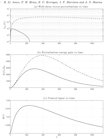
Figure 10.Linear simulation results. (a) Streamwise wall shear-stresses perturbations against time for the uncontrolled (- -) and controlled (−) flows. (b) Perturbation energy gainE(t)/E(0) against time for the uncontrolled (- -) and controlled (−) flows. (c) Controller output ˜u(t) against time. All control signals are from a weighted controller WK15 based on Re = 5000 and (α, β) := (0,2.044).
Figure 11.Velocity components and wall normal derivatives att= 293 for the controlled (–) and uncontrolled (- -) flows.
3.3. Robustness to Reynolds number variations
Figure 12.Evolution of the optimal initial condition in channel flow under the action of theH∞ loop-shaping controller. The controller is designed to attenuate the magnitude of streamwise perturbation wall shear-stresses. Filled contours represent streamwise perturbation velocities whilst vectors depict the wall-normal and spanwise velocity perturbation fields. Perturbation energy gainE(t)/E0 is also shown. Re= 5000,α= 0,β= 2.044. Notice the appearance of the buffer vortices close to the walls fort >0.
other controllers will need to be synthesised, to produce a family of controllers that can be switched between (gain-scheduled) according to the Reynolds number. Again, theν-gap
can be used to ascertain bounds on the performance degradation incurred by connecting a nominal controller to a perturbed flow.
We begin by computing the ν-gaps between the nominal 15 grid-point, Re = 5000
shaped model, denotedP5000
15,W, and a set of higher fidelity (100 grid-point) shaped models at Reynolds numbers in the range 500 6 Re 6 50,000, denoted nP100Re,W
o
. A plot
of δν
P5000
15,W,P100Re,W
is shown in Figure 14. As expected, the ν-gaps are smallest for
Figure 13.Streamwise vorticity ˜ζx att= 293 for controlled (–) and uncontrolled (- -) flows.
Figure 14.Variation of the ν-gap metric between nominal and perturbed flows. The nominal system is a 15 grid-point model based onRe= 5000,α= 0,β= 2.044. Perturbed models are based on 100 grid points and Reynolds numbers in the range 5006Re650,000.
determine the range of Reynolds numbers over which the nominal controller can be expected to perform well. For example, the robust stability margin of the loop-shaping controller from Section 3.1 was computed asbopt(P155000,W) = 0.68. Provided this exceeds theν-gap between the nominal and perturbed flows by a reasonable margin (typically
taken to be 0.3 - see Appendix A for further details) then one can expect reasonable performance from the controller. The performance requirement is thus bopt(P155000,W)−
δν
P5000
15,W,P100Re,W
[image:24.595.145.432.362.572.2]
Figure 15.Streamwise wall-shear stress perturbations against time for the uncontrolled (- -) and controlled (–) systems. Here, the controller based onP155000,Wis applied to a perturbed system of higher fidelity and higher Reynolds number,P10020,000,W.
range 500/ Re / 20,000. One would therefore expect the nominal controller to work well uponRe = 20,000 flows, and this is confirmed in Figure 15, which shows effective attenuation of the streamwise wall-shear stress perturbations for a linearised flow at this Reynolds number.
3.4. DNS results
The results from the previous section were based on a linear model of the flow, and hence neglected the nonlinearity of the Navier-Stokes equations. In this section, theH∞ loop-shaping controller is tested upon a nonlinear simulation of a channel flow. Non-linear simulations were performed using a modified version of Channelflow, a spectral DNS code for analysis of incompressible Navier-Stokes flow in channel geometries writ-ten by Gibson (2012). Velocity and pressure are represented as Fourier expansions in the periodic streamwise and spanwise directions and as Chebyshev polynomials in the wall-normal direction. Channelflow uses the influence-matrix method of Kleiser & Schu-mann (1980) to integrate the Navier-Stokes equations forward in time. This method solves the Navier-Stokes equations at each time step via solutions of a sequence of one-dimensional scalar Helmholtz equations for ˜u, ˜v, ˜wand ˜pfor each wavenumber pair, with homogenous Dirichlet boundary conditions at the walls. The code was modified in this respect to allow for inhomogeneous boundary conditions to be set at each time step by the controller. The nonlinear terms were computed in skew-symmetric format with 2/3 dealiasing in the streamwise and spanwise directions. A domain size of 4πh×2h×1.96πh, inx,y,zwas employed in all testing. The flow field was advanced in time via a third-order semi-implicit backward differentiation algorithm. Testing was performed for a range of Reynolds numbers. Grid resolutions were chosen such that ∆x+ = 12, ∆y+
min = 0.05
and ∆z+ = 7, where
·+ notation is used for values expressed in wall units. This led to
grid resolutions ranging from 184×129×158 grid points inx, y, z for the Reτ = 175
case, to 394×193×338 grid points in x, y, z for the Reτ = 360 case. Initial
Figure 16.Time evolution of the magnitude of the wall-shear stress perturbations for uncon-trolled (- -) and conuncon-trolled (–) cases. Values are normalised by the wall-shear stress magnitude at the time when the controller is switched on (t= 0).
comparing the mean velocity profiles and perturbation root-mean-square profiles from each test case to the benchmark data of Moser et al. (1999) and Iwamoto (2002). We emphasise that it was only once the flow was fully turbulent (at a nominal time t= 0) that the controllers were activated.
TheH∞loop-shaping controller was applied to aReτ= 210 flow. Figure 16 shows the
effect of this controller upon the magnitudes of the streamwise perturbation wall-shear stresses, computed for wavenumber pair (α, β) = (0,2.044). The controller was activated at timet= 0 and quickly acted to attenuate the wall shear-stress perturbations at both walls, achieving an 87% reduction in the RMS wall-shear stress perturbations. Snapshots of the controlled and uncontrolled flows are displayed in Figure 17, from which it is evident that the near-wall streaks are significantly attenuated by the action of the controller. The figure shows the appearance of buffer vortices extremely close to the wall, created by the controller. They are of just sufficient amplitude to attenuate the wall shear stress.
Further insight can be gained by studying the effects of the controller in the frequency domain. With reference to (1.3a), Figure 18 displays the gain vs frequency plots for the open and closed-loop disturbance responses,Pf and Pyf, respectively, wherePf shares
the same dynamic model as (2.8), with the exception of homogenous boundary conditions inAD and a disturbance input matrixBDof the following form:
BD:=
H−1
0
,
Com-Figure 17.Representative snapshot of the controlled (top) and uncontrolled (bottom) flows at the lower wall, taken at t = 1000. The figure shows contours of perturbation streamwise velocity (shaded regions) and perturbation streamwise vorticity (solid and dashed lines) in wall units. The near-wall streaks are significantly attenuated by the controller. The near-wall buffer vortices induce just enough streak formation of reverse sign to reduce the wall shear stress.
pared to the uncontrolled flow, the controller attenuates disturbances up to a frequency of ω = 1, just above the designed unity gain crossover frequency of the compensated system (ωc = 0.3 in Figure 8(b)). Again, and with reference to (1.5), this is to be
[image:27.595.115.439.110.388.2]Ta-10−3 10−2 10−1 100 101 10−1
100 101
ω
D
is
tu
rb
a
n
c
e
a
[image:28.595.150.403.127.324.2]m
Figure 18. Open (- -) and closed-loop (–) disturbance responses, showing the range of tem-poral frequencies over which the loop-shaping controller attenuates the worst-case disturbance forcingf, arising form the nonlinearity of the flow, upon the wall-shear stress outputy. Dis-turbance amplification is plotted in terms of ¯σ(Pf(iω)) and ¯σ(Pyf(iω)), the respective singular
value plots of the open and closed-loop transfer function matricesPf andPyf, defined in (1.3a).
Figure 19.Single-sided amplitude spectrum of the streamwise wall-shear stress perturbations forReτ= 210. The magnitudes of the wall-shear stress perturbations are significantly lower for
the controlled case (–) at frequencies below the loop crossover frequency (ω= 0.3), compared to the uncontrolled flow (- -). This is consistent with the linear system responses shown in Figure 18.
ble 1. Computational limitations limited the DNS simulations toReτ = 360 and under,
[image:28.595.165.409.401.589.2]low-Reτ = 175 Reτ = 210 Reτ = 247 Reτ = 281 Reτ = 315 Reτ = 360
87.9% 89.3% 87.5% 87.0% 88.1% 87.9%
Table 1.Percentage RMS reductions in perturbation wall-shear stresses under the control of theH∞loop-shaping controller synthesised from the nominal flow modelP155000,W.
order spatially discretised model. This is to be expected following on from the results of theν-gap analysis in Figure 14. In addition, the controller demonstrates robustness
to the dynamic uncertainty arising from the nonlinearity of the flow, providing effective regulation of the wall-shear stress despite a turbulent initial condition in which the flow is significantly perturbed away from the laminar state assumed in the control model.
4. Conclusions
We have addressed the problem of obtaining models of systems based on the Navier-Stokes equations that provide a priori robust stability and performance bounds for closed-loop flow control. It is suggested that, from the point of view of employing existing linear control systems theory, there are essentially three problems to be tackled: linearisation, spatial discretisation and conversion from a system of DAEs to one of ODEs. We have presented results that add further evidence to suggest that linear control is effective in the control of wall turbulence even though turbulence is intrinsically nonlinear. Reasons for this are encapsulated in theories such as RDT, Landahl’s ideas on sheared turbulence or gain-based analyses of turbulence formation. Specifically, by modelling the forcing arising from the nonlinearity of the flow as a disturbance input to the linear flow dynamics, we showed how the effects of such forcing could be heavily attenuated by designing a feedback controller with high loop-gain over a certain frequency range, and justified this range in terms of the timescale separation between linear and nonlinear mechanisms.
The present paper applied two methods for addressing the further issues of discretisa-tion and conversion of equadiscretisa-tions from physical to state space. For the first, the model-refinement procedure was applied to efficiently obtain spatially discretised models of low state dimension, from which robust controllers could be readily synthesised, with guaran-teed performance bounds when applied to the actual flow. This is the first instance of this technique being applied to a flow control problem. Model refinement is the conceptual opposite of model-reduction based methods, since the starting point of the former ap-proach lay with models of low, rather than high order, and where the emphasis lay upon obtaining models suitable for closed-loop, as opposed to open-loop control. This new approach to flow control employed established tools from robust control theory, such as theν-gap metric and the robust stability margin. In addition, it was argued that coprime
factor uncertainty represents an appropriate choice of uncertainty model for capturing the inevitable discrepancies that exist between an actual fluid-flow system and a simpler control model, hence motivating the use ofH∞loop-shaping control, a technique that to the best of our knowledge has not previously been applied to the problem of controlling wall turbulence. The problem of converting from physical to state space was overcome using a numerical approach that eased the prescription of boundary conditions, compared to traditional velocity vorticity-based methods.
H
address this very issue, as demonstrated by Reinschke & Smith (2003). Loop shaping design is a (temporal) frequency domain approach to control systems design. However, it should be noted that frequency does not unambiguously distinguish large structure moving quickly from small structure moving slowly, and it is the former that makes the greater contribution to skin friction. In the present work, we have assumed, for simplicity, that the walls are densely populated with sensors. As a result, the linearised system is rendered observable. Similarly, if in the control objective, small structure plays an important part in generating skin-friction drag then the techniques described in this paper ensures mesh refinement to an appropriate level by increasing the spatial fidelity of the model. Hence, the model refinement process indicates the appropriate degree of refinement required to meet the control objective. For more realistic configurations, future research should also address the consequences of non-conservative domains, i.e. those in which the nonlinearity of the disturbance field may be taken to be significant, and the extent to which it may be accommodated by the disturbance rejection framework. For flows exhibiting a more broadband forcing, such as in a turbulent mixing layer for example, our approach would require a high bandwidth controller to reject high frequency disturbances, which would likely necessitate the use of fast actuation, which may or may not be possible. The leads onto the final point that despite the potential effectiveness of the linear controllers developed in this paper, it is possible that some form of nonlinear control may provide enhanced performance by selectively exploiting the nonlinearity of the flow in some desirable fashion, and designing such controllers could be an interesting avenue of future research.
Appendix A. Quantifying the unknown with coprime factor
uncertainty
Coprime factor perturbations take the form:
Pp:=(N+UN)(M+UM)−1 , such that
UN UM ∞ < 1
γ, (A 1)
with γ > 1 and where P = N M−1 is a normalised right coprime factorisation of the unperturbed plant modelP, meaningM∗
M+N∗
N =I. The relevant block diagram is depicted in Figure 20 where the signalsv1 andv2 represent disturbances on the control
inputs u and measurements y, respectively, whilst w1 and w2 represent disturbances
acting upon the plant. The transfer functions relatingu andy, to the disturbances, are:
y u = P I
(I− KP)−1
−K I v2
v1 + I K
(I− PK)−1I
−P w2
w1
, (A 2)