Local linear embedded regression in the quantitative analysis of glucose in near infrared spectra

This is a repository copy of Local linear embedded regression in the quantitative analysis of glucose in near infrared spectra.

White Rose Research Online URL for this paper: http://eprints.whiterose.ac.uk/92964/

Version: Accepted Version

Article:

Patchava, K.C., Benaissa, M., Malik, B. et al. (1 more author) (2015) Local linear embedded regression in the quantitative analysis of glucose in near infrared spectra. Analytical Methods, 7 (4). 1484 - 1492. ISSN 1759-9660

https://doi.org/10.1039/c4ay02874k

[email protected] https://eprints.whiterose.ac.uk/ Reuse

Unless indicated otherwise, fulltext items are protected by copyright with all rights reserved. The copyright exception in section 29 of the Copyright, Designs and Patents Act 1988 allows the making of a single copy solely for the purpose of non-commercial research or private study within the limits of fair dealing. The publisher or other rights-holder may allow further reproduction and re-use of this version - refer to the White Rose Research Online record for this item. Where records identify the publisher as the copyright holder, users can verify any specific terms of use on the publisher’s website.

Takedown

If you consider content in White Rose Research Online to be in breach of UK law, please notify us by

Local Linear Embedded Regression in the Quantitative Analysis of Glucose in Near

Infrared Spectra

1

Krishna Chaitanya Patchava, 1Mohammed Benaissa, 1Bilal Malik, 2Hatim Behairy

1

Department of Electronic and Electrical Engineering, The University of Sheffield, Portabello centre, Sheffield S1 4DR, United Kingdom

2

National Electronics, Communication and Photonics Center, King Abdulaziz city for Science and Technology (KACST), Riyadh 11442, Saudi Arabia.

[email protected]@sheffield.ac.uk [email protected] [email protected]

Abstract

This paper investigates the use of Local Linear Embedded Regression (LLER) for the

quantitative analysis of glucose from near infrared spectra. The performance of the LLER model is evaluated and compared with the regression techniques Principal Component

Regression (PCR), Partial Least Squares Regression (PLSR) and Support Vector Regression (SVR) both with and without pre-processing. The prediction capability of the proposed model has been validated to predict the glucose concentration in an aqueous

solution composed of three components (urea, triacetin and glucose). The results show that the LLER method offers improvements in comparison to PCR, PLSR and SVR.

Keywords: LLER, glucose, NIR, DBPF, Chebyshev bandpass filter, Gaussian bandpass

1. INTRODUCTION

Diabetes mellitus is a chronic disease that is increasing at an alarming rate [1]. Diabetic patients must monitor their blood glucose levels several times a day in order to have better

control of their condition. The conventional technique for measuring glucose levels is the finger prick method, which is very painful and inconvenient on a daily basis. To address

this issue, researchers have tried to come up with non-invasive techniques for glucose measurement.

Near Infrared (NIR) spectroscopy has been identified as one of the promising techniques

for non-invasive glucose measurement. NIR spectroscopy is faster and provides a reasonable signal-to-noise ratio as compared to other methods. The prediction of the

concentration of glucose from a NIR spectra remains a challenge due to underlying noise and necessitates the development of advanced and efficient multivariate data analysis algorithms [2-5].

Principal Component Regression (PCR) and Partial Least Squares Regression (PLSR) are the most commonly used multivariate regression methods for the quantitative analysis of

NIR absorbance spectra [6-11]. However, these models degrade prediction performance if the analyte of interest contributes less variation to the spectra [12]. The drawbacks of the PCR and PLSR models mentioned above motivated the implementation of a new regression

model which preserves the information related to an analyte of interest irrespective of its variation in the spectral mixture.

a non-linear dimensionality reduction technique called Local Linear Embedding (LLE) [13] is used to map the high dimensional data non-linearly into a low dimensional space. Due to its advantages such as no local minima, good representational capacity and high

computational efficiency, LLER is considered one of the robust regression models for non-linear data [14].

In this paper, the LLER model is first developed and then evaluated and compared to key existing regression techniques. Pre-processing methods in terms of first-derivative and bandpass filtering are also implemented with the different regression methods and the

resulting models are evaluated. It is shown that the LLER technique can be an attractive alternative model for the prediction of glucose from NIR spectra.

2. THEORY

2.1 Local Linear Embedding (LLE) Dimensionality Reduction Algorithm:

An LLE analysis on a raw matrix consisting of N vectors with dimensionality D can be

implemented as follows:

Let the number of nearest neighbours and the dimensionality of the embedded data be K and

d respectively. Initially, K-nearest neighbors of each data point are identified by using

Euclidean metric and the reconstruction weights that best represent the data points by

their neighboring points can be computed by minimizing the following cost function E(W).

2 1 1 ) (





i W X

X W

E   (1)

i

X

ij

where the reconstruction weights signify the contribution of the j’th point to the i’th

reconstruction. The cost function also represents the reconstruction error, which is the

squared sum of the difference between the actual data and the reconstructed data. The cost function can be minimized with the following two constraints:

The first constraint is the sum of all the reconstruction weights should be equal to unity. i.e.

.

The latter constraint is every data point is reconstructed only from its neighbouring points.

i.e.

=0, if Xj is not one of the K nearest neighbouring points. The significance of these two constraints is that for any particular data point, the reconstruction weights are invariant to rescalings, rotations and translations of that data point and its neighbours. The invariance to

translations is achieved by the first constraint [13].

Solving equation (1) based on the above constraints is a least square problem as given in [13]. The optimum weights are invariant to translation, rescaling and rotation of the data

point and its neighbours.

Finally, the embedded vector , with dimensionality equal to d can be computed by

minimizing the local reconstruction error _.

(2) ij W 1 1 







i WY

Y

where _{is the local reconstruction error that represents the summed squares of the}

difference between the original embedded data and their reconstruction and are the

reconstruction weights calculated from equation (1).

The local reconstruction error can be reduced with the following two constraints:

1.

2.

where I represents an identity matrix.

Solving, the embedded vector is a well-known problem in linear algebra and it can be minimized by solving the sparse N×N Eigen vector problem [13].

The advantage of the algorithm is that the LLE model has to set only one parameter K which affect the performance of the LLER model in a direct way. However, incorrect choice of K may degrade the performance of the model. If the value of K is selected too small, the

mapping loses its global property [15]; on the other hand, if the value of K is selected too high, the data mapping will lose its non-linear property [16].

Two methods are proposed to optimize the neighbourhood size (K) in [16]. In the first method, the residual variance of the embedded data is calculated for every value of K in the

range [1- ]. The optimum value is the value of ‘K’ corresponding to minimum

residual variance. The limitation of this method is that it is time consuming, as it needs to

optimize both the reconstruction error E(W) and the local reconstruction error _for ) (Y  ij W ) (Y  0 1 





1  

max

K K_opt

every value of K. In the second method, the cost function E(W) is calculated for different

values of K in the range [1- ], which is called hierarchical method; K_opt corresponds

to the minimum residual variance. However, the residual variance has more than one minimum [16] resulting a set S of potential candidates for K_opt. Residual variance must be computed for each value of K from the set S. The value of K corresponds to the minimum

residual variance is chosen as K_opt.

The first method is used to optimize the parameter K in this study.

2.2. Local Linear Embedded Regression (LLER):

In the LLER method, the LLE analysis is used to map the high dimensional absorbance spectra (A) to a lower dimensional embedded vector (Y).

The absorbance matrix A is decomposed as the product of the Local Linear

Embedding matrix Y and the reconstruction factors P.

A=Y.P (3)

where d is the dimensionality of the embedded vector, N is the number of training spectra,

and D is the number of variables in the raw spectra.

In the LLER method, the scores actually represent the embedded vectors that are computed

from the LLE algorithm and then the loading matrix is computed by multiplying the pseudo-inverse of the scores matrix with the input raw spectra. The obtained scores and loading matrices can be used in building the LLER model.

The reconstruction matrix can be represented as shown in equation (4).

max

K

D N  

(4)

where _{is the pseudo-inverse of the embedded data matrix Y. Embedded vector Y and}

reconstruction factors P are considered to be scores and loading factors respectively. As the concentration of analyte (Cg) relates to the embedded data Y, the embedded data can be regressed against the analyte’s concentration using Multiple Linear Regression (MLR) as

follows.

Cg=Y. lle (5)

Where lle _{represents the coefficients of the regression.} lle _{is defined by the least squares} method as

(6)

The concentration for the new data can be obtained from the following equation,

when both the training spectra and concentration are centered.

C_gnew (A_newA)C_g (7)

From equatons 3 and 5, can be replaced by lle

(8)

where is the pseudo-inverse of the loading factors of the training spectra, _{is the}

average vector of the training spectra and is the average value of the training data

concentration.

A

Y P  



Y

g lle  YY YC

1 ) ( 

gnew

C A_new



P

g lle new

gnew A A P C

C (  )  



P A

g

As explained above, the LLER model has to set two parameters, one is the K nearest neighbouring points and the other one is the dimension of the embedded data d. If d is selected too high, the mapping reduces the signal-to-noise ratio; conversely, if d is selected

too small, different parts of the dataset might be mapped onto each other [17]. The lower and upper limits of K are chosen as the minimum and maximum possible values of K for which

the LLER model converges.

The implemented calibration models are tested by using the test dataset. For each value of K, the error parameters Root Mean Square Error of Calibration (RMSEC), Root Mean Square

Error of Cross Validation (RMSECV) and RMSEP are computed. The values of d and K that together produce the minimum RMSECV are selected as the optimum parameters of the

LLER calibration model.

2.3 LLER model Combined with Digital Bandpass Filtering

The performance of the calibration model can be improved by the integration of the LLER

model with pre-processing techniques such as the first derivative and bandpass filtering. To our knowledge, this is the first time LLER is combined with digital bandpass filtering for NIR spectroscopy. In this work, the digital Gaussian and Chebyshev bandpass filters have

been used to suppress the high frequency components as well as the baseline variations which dominate the low frequency components in the raw spectra [18,19]. The digital

A Gaussian filter can be implemented either in the frequency domain or in the time domain. The Gaussian function has the same profile in both the frequency and time domains [22,23]. In the frequency domain, the mean and standard deviation of the Gaussian function are

equivalent to the centre frequency and bandwidth respectively. The Gaussian bandpass filter was implemented in the frequency domain, as shown in Figure 1, due to its reduced

complexity.

Figure 1: Block diagram of the Gaussian digital bandpass filter

Initially, the Fast Fourier Transform is applied on the input raw spectra, which is then multiplied with the Gaussian function; the input to the Gaussian function is the raw spectra

Chebyshev filters provide an optimal tradeoff between passband ripples and a steeper roll- off, compared to other time domain filters [24] and can be efficiently implemented in time domain. The block diagram of the Chebyshev digital bandpass filter is shown in Figure 2

below.

Figure 2: Block diagram of the Chebyshev digital bandpass filter

Initially, an analog low pass filter is designed, with the upper cut-off frequency equal to half of the desired bandwidth of the Digital Bandpass (DBP) filter. The obtained low pass filter is

transformed to a bandpass filter by shifting the spectrum to the centre frequency of the DBP filter. The transfer function in analog form is then converted to the digital domain by

obtained by applying the inverse Z-transform on the previous output. Finally, the raw spectra is convoluted with the impulse response of the Chebyshev filter to obtain the filtered signal.

The grid search optimization [25] is used to optimize the filter parameters. Initially the RMSECV is calculated for all possible values of centre frequency and bandwidth. The

predictive performance of the models is evaluated by using the coefficient of determination (R2), the Root Mean Square Error of Calibration (RMSEC), the Root Mean Square Error of Cross Validation (RMSECV) in addition to the Root Mean Square Error of Prediction

(RMSEP). A good model should have a high R2, a low RMSEC, a low RMSECV, and a low RMSEP. The optimum values of c and w are selected as the values of c and w for which the

RMSECV has the minimum value.

3. Experimental data preparation

For this experiment, samples were prepared by dissolving glucose, urea and triacetin in a

phosphate buffer solution. Triacetin was used to model the triglycerides in the blood. Dry solutes of glucose and urea were dissolved in the buffer to prepare their aqueous solutions whereas triacetin solution was diluted by the buffer solution. The buffer solution was

prepared by dissolving 3.4023 grams of potassium dihydrogen and 3.0495 grams of sodium mono hydrogen phosphate in distilled water. A preservative in the form of

fluorouracil was added to the buffer solution. The analytes used in this experiment were purchased from Sigma Aldrich, UK.

within physiological range in blood. Concentration of glucose, urea and triacetin ranged from 20 to 500 mg/dL, 0 to 50 mg/dL and 10 to 190 mg/dL respectively. After preparing the samples, triplicate spectra for each sample were collected with a Fourier transform

spectrophotometer (spectrophotometer Cary 5000 version 1.09) which spanned the spectral region from 2000 nm to 2500 nm with a spectral resolution of 1 nm and in this way 90 NIR

spectra were collected from 30 samples. The purpose of using three replicate spectra is to reduce the effect of instrument noise. The absorbance spectra of the buffer solution were

used as reference spectra.

The collected spectra were divided randomly into calibration and test sets. The calibration set contained the three replicate spectra of 20 samples and was used to build the calibration

model. The test set contained the triplicate spectra of 10 samples and was used in the prediction phase to test the calibration model.

The experiments were carried out in a non-controlled environment. i.e; experiments were

not carried under constant temperature. This introduced significant baseline variation in the collected spectra to evaluate the ability of the proposed methods in this work to deal with

the uncompensated variations. Many previous studies in this area have carried out experiments in a controlled environment to compensate the effect of the baseline variation.

In this study, the Van Der Maaten toolbox [26] has been used to perform the LLE

overfitting problem. The doublet (K,d) with the lowest RMSECV is used to build the final LLER model. The optimum number of PCs and LVs for the PCR and PLSR models were

found using “10-fold cross validation” respectively. The key parameters for SVR model

using Radial Basis Fucntion (RBF) kernel are cost (C), gamma () and epsilon (). The grid search optimization on C,  and  using 10-fold cross validation was used to avoid over

fitting problem as mentioned in LIBSVM (A Library for Support Vector Machines) [27]. The triplet with minimum RMSECV were chosen as the optimum parameters to build the

final SVR model.

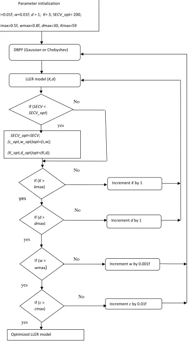
The grid search optimization [25] is used to optimize the filter parameters (c,w). In the optimization of the DBP filtering, the centre frequency (c) is varied from 0.01 f to 0.5 f and

the bandwidth (w) is varied from 0.01 f to 0.8 f; where f is the normalized frequency [19]. The values for the filter parameters (c and w) are chosen in such a way that the filter spans the whole frequencies from fL= (c-w/2) to fH= (c+w/2); where fL is the lower cutoff frequency and fH is the upper cuttoff frequency of the designed digital bandpass filter. In each iteration, the designed digital bandpass filter is combined with the prediction model

and the RMSECV is calculated. The computed RMSECV is then stored in the variable called SECV and is compared with SECV_opt as shown in the flowchart below; where SECV_opt is the temporary variable used to store the updated minimum RMSECV value in

Parameter initialization

c=0.01f; w=0.01f; d = 1; K= 3; SECV_opt= 200;

cmax=0.5f, wmax=0.8f, dmax=30, Kmax=59

Optimized LLER model

DBPF (Gaussian or Chebyshev)

LLER model (K,d)

If (d > dmax)

If (c > cmax) If (w >

wmax)

If (K > kmax) If (SECV < SECV_opt)

Increment K by 1

Increment d by 1

Increment w by 0.001f

Increment c by 0.01f SECV_opt=SECV;

(c_opt,w_opt)opt=(c,w); (K_opt,d_opt)opt=(K,d); yes No yes No yes yes yes No No No

the c_opt, w_opt, K_opt, d_opt respectively. The maximum values for c, w, K and d are considered as cmax, wmax, Kmax, and dmax respectively. The prediction model with the lower RMSECV is chosen as the optimized digital bandpass filter. The optimum filter

parameters for the Chebyshev filter are found to be c=0.03 f, w= 0.04 f and for the Gaussian digital filter, these were c= 0.02 f, w=0.01 f .

The selection process of the parameters for the optimum DBPF-LLER model is illustrated in the flow chart as shown in Figure 3.

4. Discussion of Experimental Results and Comparisons:

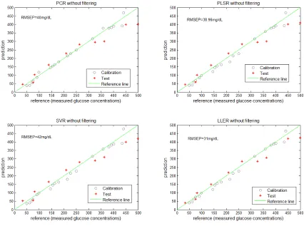
For the evaluation, validation, and comparisons, a set of prediction models were developed. Initially the PCR, PLSR, SVR and LLER models were implemented with no

pre-processing. The prediction performance of the models was examined by computing the RMSEP, RMSEC, RMSECV and R2 for each model. Figure 4 shows the comparison of all the prediction models with no pre-processing; the x-axis shows the reference glucose

concentration (mg/dL) and the y-axis represents the predicted glucose concentration

(mg/dL). The ‘*’ symbols correspond to the test samples where as ‘o’ symbols correspond

Figure 4: Comparison of the PCR, PLSR, SVR and LLER models without pre-processing

The results demonstrate that the LLER model gives a better prediction compared to the

PCR, PLSR and SVR models when no pre-processing of the raw data is used. This is an interesting result that confirms the advantage of adopting an efficent non-linear dimensionality reduction technique (LLE) in a calibration model when dealing with NIR

spectra. Figure 4 shows that the LLER model exhibits a more consistent precision of calibration relative to the PCR, PLSR and SVR models, although the testing and training

coordinates into low dimensional data (Y) by minimising the cost function (Y)as given in

equation 2. The cost function is based on the reconstruction coefficients of K nearest neighbours. Then the mapped data are regressed against the analyte of interest to build the calibration model, which is completely identified by the embedded dimension d and the K

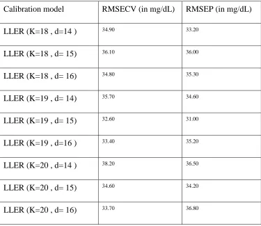
nearest neighbours. So, the values of K and d affect the prediction performance of the LLER model. This has been investiagted and Table 1 below summarises the impact of

these two parameters on the resulting RMSEP and RMSECV values for the LLER model.

Table 1: The prediction capability of the LLER model for different values of K and d

Calibration model RMSECV (in mg/dL) RMSEP (in mg/dL)

LLER (K=18 , d=14 ) 34.90 33.20

LLER (K=18 , d= 15) 36.10 36.00

LLER (K=18 , d= 16) 34.80 35.30

LLER (K=19 , d= 14) 35.70 34.60

LLER (K=19 , d= 15) 32.60 31.00

LLER (K=19 , d=16 ) 33.40 35.20

LLER (K=20 , d=14 ) 38.20 36.50

LLER (K=20 , d= 15) 34.60 34.20

Furthermore, as already mentioned, appropriate pre-processing of the raw data prior to applying the calibration model can yield tangible improvements in prediction, since the raw NIR spectra are affected by baseline shift, background noise, light scattering and

instrumental noise in general. Hence, a set of pre-processing techniques including first derivative, Gaussian digital bandpass filtering and Chebyshev digital bandpass filtering are

applied and evaluated for each model.

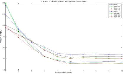
Firstly, the PCR and PLSR models were implemented with the different pre-processing techniques where the number of factors that produce the minimum RMSECV are chosen as

the optimum number of principal components and latent variables for PCR and PLSR respectively. The comparison of PCR and PLSR when different pre-processing techniques

are applied is shown in Figure 5. The y-axis shows the RMSECV and the x-axis represents the number of principal components or Latent variables for PCR and PLSR respectively. The results show that the models with pre-processing of NIR data gives much better

prediction accuracy in comparison to models with no pre-processing. From Figure 5, it is also observed that models with bandpass filtering achieve better prediction accuracy in

comparison to the first derivative pre-treatment. The optimum number of principal components and latent variables are identified to be 6. Information about NIR spectra is prominent in the frequency components in the mid-band range, while the noise and baseline

variations tend to occupy the high and the low frequency range respectively, that is why these can be effectively reduced using an optimised bandpass filter rather than the first

filter can eliminate both the low frequency baseline variations and the high frequency noise from the spectra.

The PCR, PLSR, SVR and LLER models were then implemented with the raw data

pre-processed using the first derivative, the Gaussian, and the Chebyshev digital bandpass filters.

Figure5: PCR and PLSR with different pre-processing techniques

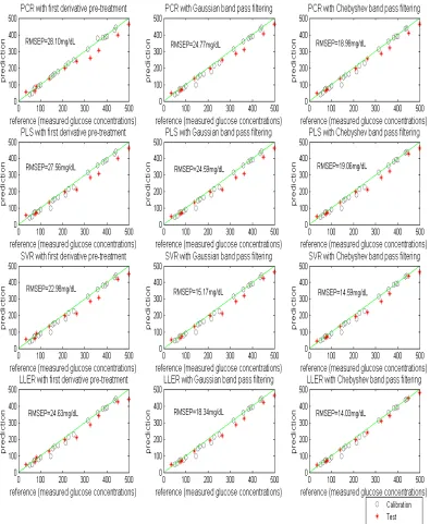
Figure 6 illustrates the prediction performance comparison of the PCR, PLSR, SVR and

LLER models with the three different pre-processing methods. For each subplot, the x-axis represents the reference glucose concentration (mg/dL) and the y-axis shows the predicted glucose concentration (mg/dL). The ‘o’ symbols correspond to the calibration where as ‘*’

combined with the Chebyshev filter gives the best prediction accuracy. The advantage of a Chebyshev filter over a Gaussian bandpass filter is that it offers an optimal trade off between a steeper roll off and passband ripples. Hence, it is more effective in reducing the

Table 2 Comparison of PCR,PLSR, SVR and LLER models

Regression

model

Pre

processing

Optimum parameters RMSEC* RMSECV* RMSEP*

PCR None 6PCs 25.34 67.59 0.90 40.00

PCR 1st

derivative

6PCs 24.92 51.07 0.88 28.10

PCR GDBPF 6PCs 17.54 56.70 0.97 24.77

PCR CDBPF 6PCs 15.93 51.23 0.98 18.98

PLS None 6LVs 11.30 34.07 0.90 38.96

PLS 1st

derivative

6LVs 22.54 31.59 0.97 27.56

PLS GDBPF 6LVs 12.00 38.30 0.96 24.59

PLS CDBPF 6LVs 15.92 28.43 0.98 19.06

SVR None  C= 0.1*10^6 2.50 38.44 0.90 42.00

SVR 1st

derivative

 C= 0.2*10^6 13.50 28.98 0.98 22.98

SVR GDBPF  C= 0.04*10^6 12.09 28.00 0.99 15.17

SVR CDBPF  C= 4.5*10^6 12.47 27.40 0.99 14.59

LLER None K=19, d=15 18.52 32.60 0.95 31.00

LLER 1st

derivative

K=29, d=25 15.55 31.50 0.97 24.63

LLER GDBPF K=33, d=20,

c=0.03f, w=0.04f

14.92 27.80 0.98 18.34

LLER CDBPF K=55, d=23

C=0.02f, w=0.01f

*=(units are in mg/dL);GDBPF=Gaussian digital bandpass filter;CDBPF=Chebyshev digital bandpass filter.

5. Conclusions

In this paper, the use of the LLER method is investigated for the prediction of glucose concentration from near infrared spectra. The prediction capability of the proposed model

has been evaluated and validated to generate and predict the glucose concentration of aqueous solutions composed of urea, triacetin and glucose. The results show that the LLER model outperforms PCR, PLSR and SVR models without pre-processing and show that the

digital bandpass filter pre-processing could improve the prediction performance of the PCR, PLSR, SVR and LLER models in Comparison to the first derivative pre-treatment.

The prediction capability of the LLER model is quite sensitive to the dimension of the embedded data (d) and the number of nearest neighbor points (K). Hence the selection of these parameters is very important to get the optimum results.

REFERENCES

1. Diabetes, U. K. "Diabetes in the UK 2010: key statistics on diabetes. 2010." URL: www.

diabetes. org. uk/Documents/Reports/Diabetes_in_the_UK_2010. pdf (accessed 22 March

2012) .

2. Wabomba, Mukire J., Gary W. Small, and Mark A. Arnold. "Evaluation of selectivity and

robustness of near-infrared glucose measurements based on short-scan Fourier transform

infrared interferograms." Analytica Chimica acta, 490.1 (2003): 325-340.

3. Al-Mbaideen, Amneh A., Tanzilur Rahman, and Mohammed Benaissa. "Determination of

glucose concentration from near-infrared spectra using principle component regression

coupled with digital bandpass filter." Signal Processing Systems (SIPS), 2010 IEEE

Workshop on. IEEE, 2010.

4. Robinson, M. Ries, et al. "Noninvasive glucose monitoring in diabetic patients: a preliminary

evaluation." Clinical Chemistry 38.9 (1992): 1618-1622.

5. R.W. Waynant, V.M Chenault, “Overview of Non Invasive Fluid Glucose measurement

using optical techniques to maintain Glucose control in Diabetes Mellitus’’,

IEEE.org/organizations/pubs/newsletters/leos/apr98/overview.htm.

6. I.T Jollife, “Principal Component Analysis”, Second edition, springer 2002.

7. R.Kramer, ”chemometrics techniques for quantitative Analysis”, Marcel-Dekker (1998).

8. Amneh Al-Mbaideen, Mohammed Benaissa, “Determination of glucose concentration from

NIR spectra using Independent component regression”, Chemometrics and Intelligent

laboratory systems, 105, pp 131-135,2011

9. Haaland, David M., and Edward V. Thomas. "Partial least-squares methods for spectral

analyses. 1. Relation to other quantitative calibration methods and the extraction of

qualitative information." Analytical Chemistry 60.11 (1988): 1193-1202.

10. Donald A. Burns, Emil W Ciurczak, “Handbook of Near Infrared Analysis,” Taylor and

11. Lin Zhang, Gary W. Small and Mark A. Arnold “ calibration standardization algorithm for

partial Least Squares Regression: Application to the determination of physiological levels of

glucose by Near-Infrared spectroscopy,” Analytical.Chemistry.2002,74,pp 4097-4108.

12. Yazdani, Samaneh, Jamshid Shanbehzadeh, and Mohammad Taghi Manzuri Shalmani.

"RPCA: a novel preprocessing method for PCA." Advances in Artificial Intelligence 2012

(2012).

13. Roweis, Sam T., and Lawrence K. Saul. "Nonlinear dimensionality reduction by locally

linear embedding." Science 290.5500 (2000): 2323-2326.

14. Vin de silva and Joshua B. Tenenbaum, “Global versus Local methods in Non linear

Dimensonality Reducton,” proceedings of the conference on Advances in Neural Informaton

Processng Systems (NIPS), 2003.

15. Dick de Ridder and Robert P.W. Duin, “Locally Linear Embedding for classification,” IEEE

transactions on pattern Analysis and Machine Intelligence. http://www.ph.tn.tudelft.nl/~dck

16. Olga Kouropteva, Oleg Okun and Matti pietik , “Selection of the optimal parameter value for

the Locally Linear Embedding algorithm,” In: Proc of the 1st International conference on

Fuzzy Systems and Knowledge Discovery (FSKD’02),pp.359-363.

17. de Ridder, Dick, and Robert PW Duin. "Locally linear embedding for classification."Pattern

Recognition Group, Dept. of Imaging Science & Technology, Delft University of Technology,

Delft, The Netherlands, Tech. Rep. PH-2002-01(2002): 1-12.

18. Gary W. Small , Mark A. Arnold and Lois A. Marquadt, “Strategies for coupling Digital

filtering with partial Least Squares Regression: Application to the determination of glucose

in plasma by Fourier Transform Near- Infrared spectroscopy,” Analytical Chemistry

1993,65,pp 3279-3289.

19. Ham, Fredric M., et al. "Determination of glucose concentrations in an aqueous matrix from

NIR spectra using optimal time-domain filtering and partial least-squares

20. Mitra, Sanjit KK. ‘’Digital signal processing: a computer-based approach’’. McGraw-Hill

Higher Education, 2000.

21. Parks, Thomas W., and C. Sidney Burrus. Digital filter design. Wiley-Interscience, 1987,.

22. Oppenheim, Alan V., Ronald W. Schafer, and John R. Buck. Discrete-time signal

processing. Vol. 5. Upper Saddle River: Prentice hall, 1999.

23. Smith, S. W. Digital signal processing: a practical guide for engineers and scientists.

Newnes,2003.

24. Belle A. Introduction to digital signal processing and filter design. Wiley-Interscience, 2005.

25. Arnold, Mark A. "Non-invasive glucose monitoring." Current opinion in biotechnology 7.1

(1996): 46-49.

26. Van der Maaten toolbox for dimensionality reduction

http://homepage.tudelft.nl/19j49/Matlab_Toolbox_for_Dimensionality_Reduction.html

27. Chang, Chih-Chung, and Chih-Jen Lin. "LIBSVM: a library for support vector