A computer simulation of ST segment shift in myocardial ischaemia

(1)

Division of Clinical Sciences

U•iversity-of-Tasmania

April 7, 1998

Segment Shift in Myocardial

Ischaemia

Chuan Yong Li

BSc., MSc.

(2)

Declaration

The investigations described in this thesis constitute my own work. This thesis con-tains no material which has been accepted for the award of any other higher degree or graduate diploma in any tertiary institution. To the best of my knowledge and belief, this thesis contains no material previously published or written by another person, except where due acknowledgement and reference are made in the text of the thesis.

Signed:

Date: October, 1997

This thesis may be made available for loan and limited copying in accordance with the Copyright Act 1968.

Signed:

(3)

This thesis presents a computer simulation of electrocardiographic ST segment shift in myocardial ischaemia to elucidate the source of ST changes in both subendocardial and transmural ischaemia.

A realistic torso model was constructed, in which the myocardium was represented by the bidomain model. In a normal heart, there is no current source during the ST segment and there is a minimal ST potential field. With myocardial ischaemia, the transmembrane potential of ischaemic cells changes, allowing current to flow between the ischaemic and nonischaemic regions, which generates ST segment shift. The ischaemic regions included in the model were those measured using fluorescent microspheres in a sheep model, and the transmembrane potentials were generated from values extracted from the literature.

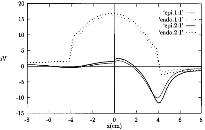
Subendocardial ischaemia in the territory supplied by either the left anterior de-scending coronary artery (LAD) or left circumflex coronary artery (LOX) was simu-lated, showing that the current source is produced at the ischaemic boundary, with the positive source at the ischaemic and the negative source at the normal side of the boundary. At the intramural boundary, the current flow is highly localised around the boundary, while at the lateral boundary normal to the endocardium, current flows both by crossing the boundary and through the intracavity blood. Epicar-dial ST depression is seen over the lateral boundary while endocarEpicar-dial ST elevation appears over the ischaemic region. The source in the septum is not seen on the epicardium because it is surrounded by highly conductive blood. LAD and LCX ischaemia share the lateral boundary and produce a similar pattern of epicardial ST depression on the left free wall.

Transmural ischaemia of varying size was studied. Transmural ischaemia of a small region produces localised ST elevation over the ischaemic region with little ST de-pression elsewhere on the epicardium and a similar pattern on the endocardium with a much lower amplitude. Ischaemia in either the LAD or LCX territory produces a strong dipole on the epicardium over the left lateral region, with ST elevation on the ischaemic region and ST depression on the nonischaemic region. ST depression in transmural ischaemia is generated with ST elevation and is an integral part of the source, thus it is inevitable that ST depression on the body surface will be generated during ischaemia of a large region of myocardium.

The effect of the myocardial anisotropy on ST potentials was also studied. The inclusion of myocardial anisotropy produces results somewhat closer to measured results in animal models.

(4)

Acknowledgements

I wish to sincerely thank my supervisor, Professor David Kilpatrick, for his constant

guidance, invaluable advice and encouragement throughout the whole project.

I also wish to thank my husband Mr. Desheng Han and my son Li Han for their

continuous support and encouragement during these years, without which this task

would have been much more difficult.

I am grateful to Dr. Danshi Li and Dr. Timothy Gale for their kind help in providing

the related data used in this thesis.

Grateful thanks are also extended to:

Dr. Peter Johnston for his technical assistance.

Dr. Ah Chot Yong, Dr. Yong-shun Xiao, Mr. Kevin Pullen, Mrs Julia Greenhill, Mr.

Malcolm Johnson, Mrs Sue Johnson and Mrs Margaret Wright for their language

aid and proof-reading.

Professor G. W. Boyd and Dr. Janet Vial for providing the opportunity to undertake

this work in the Discipline of Medicine, and also my colleagues and staff in this

Department and Clinical School for providing a congenial and friendly atmosphere

to work.

Tianjin Medical University and the Ministry of Education in China for providing

the opportunity to study in Australia.

I would like to acknowledge the financial support received from the Australian

Agency for International Development (AusAID).

Special thanks go to my parents and my parents in-law for their support and

un-derstanding.

(5)

(6)

Publications

Full papers

• C. Y. Li, W. K. Pluta and D. Kilpatrick, Field Programmable Gate Array in a fast 256-channel data acquisition system, Australasian Physical & Engineering Sciences in Medicine, Vol. 20, No. 1, P47-52, 1997

Short papers/Abstracts

• C. Y. Li, D. S. Li, D. Kilpatrick and P. R. Johnston, A computer model of ST depression in transmural ischaemia, 45th Annual Scientific Meet-ing of the Cardiac Society of Australia and New Zealand, Hobart, Tasmania, Australia, 10-13 August, 1997, P229

• C. Y. Li, D. S. Li, D. Kilpatrick and P. R. Johnston, An explanation for ST depression in subendocardial ischaemia, 45th Annual Scientific Meeting of the Cardiac Society of Australia and New Zealand, Hobart, Tasmania, Aus-tralia, 10-13 August, 1997, P230

• L. Wang, C. Y. Li, A. C. Yong and D. Kilpatrick, Determination of mean ventricular fibrillation intervals as an index of ventricular refrac-toriness: fast Fourier transform analysis versus time averaging tech-nique, 45th Annual Scientific Meeting of the Cardiac Society of Australia and New Zealand, Hobart, Tasmania, Australia, 10-13 August, 1997, P272

• L. Wang, C. Y. Li, A. C. Yong and D. Kilpatrick, The effect of acute myocardial ischaemia on ventricular refractoriness and its dispersion in sheep, 45th Annual Scientific Meeting of the Cardiac Society of Australia and New Zealand, Hobart, Tasmania, Australia, 10-13 August, 1997, P47 • C. Y. Li, D. Kilpatrick, P. R. Johnston,. and D. S. Li, A bidomain model of

ST changes during subendocardial ischaemia, 18th Annual International Conference of the IEEE Engineering in Medicine and Biology Society, 1996, Track 5.4.1, Paper number:1083

• C. Y. Li, W. K. Pluta and D. Kilpatrick, A fast 256-channel data

ac-quisition system, Engineering and Physics in Medicine, Queenstown, New Zealand, 20-24 November, 1995, P199

(7)

3D three dimensional

AP action potential

BSPM body surface potential maps

DC direct current

CT computerised tomography

ECG electrocardiogram

EMF electromotive force

FDM finite difference method

FEM finite element method

FIDAP fluid dynamics analysis package

LAD left anterior descending coronary artery

—

LCX left circumflex coronary artery

LV left ventricle

LVC left ventricular cavity

LVW left ventricular wall

MRI magnetic resonance imaging

OM obtuse marginal branch of the left circumflex coronary artery

FDA posterior descending coronary artery

PTCA percutaneous transluminal coronary angioplasty

RCA right coronary artery

RMBF regional myocardial blood flow

RMS root mean square

RV right ventricle

SI spatial intracellular

SPT septum

VCG vectorcardiogram

(8)

5 Simulation of subendocardial ischaemia

74

5.1 Introduction 74

5.2 Simulations 75

5.3 FIDAP solution 79

5.4 Results 79

5.5 Discussion 90

5.5.1 Epicardial ST depression does not localise subendocardial ischaemia while endocardial ST elevation does 90

5.5.2 Current source 94

5.5.3 Ischaemic boundaries 95

5.5.4 Current path 96

5.5.5 ST potential on the body surface 97

5.5.6 Transition to full thickness ischaemia 98

5.5.7 Solid angle theory 99

5.5.8 Blood effect 100

5.5.9 Effect of torso tissues 101

5.5.10 Clinical implications 101

5.5.11 Conclusion 102

5.5.12 Evaluation of the source approximation 102

5.5.13 Limitations 103

6 Simulation of transmural ischaemia

104

6.1 Introduction 104

(11)

CONTENTS

6.2.1 3D block model

6.2.2 Isolated heart model

6.2.3 Torso model

x

106

108 6.3 Transmural ischaemia of a large region

108 6.3.1 3D block model

109 6.3.2 Isolated heart model

109 6.3.3 Torso model

111 6.4 FIDAP solution

111 6.5 Results

111 6.5.1 Transmural ischaemia of a small region

111 6.5.2 Transmural ischaemia of a large region

117 6.6 Discussions

121 6.6.1 Current source

121 6.6.2 Current path

125 6.6.3 ST elevation distribution over ischaemic region 127

6.6.4 Amplitude of ST elevation and size of ischaemic region . 130

6.6.5 ST depression in transmural ischaemia

131 6.6.6 Comparison with previous models

133 6.6.7 Clinical implications

135 6.6.8 Limitations

136

7 Effects of myocardial anisotropy 137

7.1 Introduction

137 7.2 Myocardial anisotropy

138 7.3 Simulations

139 7.3.1 Subendocardial ischaemia

139 7.3.2 Transmural ischaemia of a small region

140 7.3.3 Transmural ischaemia of a large region

141 7.4 FIDAP solution

142

(12)

Introduction

Electrocardiographic ST segment shift is a marker of myocardial ischaemia, and is generated by electrical currents flowing across the ischaemic boundary due to changes in the transmembrane potential of the ischaemic muscle. It provides some information about the location and the severity of the ischaemic injury, but its clin-ical usefulness is limited because some of the clinclin-ical and experimental observations can not be explained by the classic models of ST segment shift.

It is well known that ST depression can not localise the underlying ischaemic re-gion in subendocardial ischaemia [1, 2, 3, 4], but the mechanism is unclear [5]. There are also controversial reports regarding the distribution pattern and the am-plitude of ST potential varying with the ischaemic size during transmural ischaemia (infarction) [6]. Small regions of transmural ischaemia tend to produce uniform epicardial ST elevation over the ischaemic region with little ST depression over the adjacent non-ischaemic region [7, 8, 9]. Large regions of ischaemia produce epicar-dial ST elevation with its amplitude not correlating with the underlying ischaemic region [10, 11, 12, 13], and ST depression over the non-ischaemic region [14, 7, 15]. ST depression on the body surface also occurs in patients with acute infarction [16, 17, 18, 19]. However, the mechanism which causes this ST depression in in-farction remains controversial [20]. A study in which simultaneous endocardial and epicardial ST potentials were mapped in sheep was conducted by Li in our labo-ratory [21]. Ischaemia was produced by atrial pacing and coronary artery ligation,

(14)

CHAPTER 1. INTRODUCTION

and confirmed by blood flow measurement using the fluorescent microsphere

tech-nique. In Li's study, mapping was performed in the following five types of ischaemia:

subendocardial ischaemia in the territory of either the left anterior descending

coro-nary artery (LAD) or the left circumflex corocoro-nary artery (LCX), and transmural

ischaemia in the territory of the obtuse marginal branch (OM) of the LCX, the

LAD and the LCX.

The aim of this thesis is to simulate ST potentials in ischaemia and to derive current

paths which will elucidate Li's experimental results and related clinical observations.

Three different models, a 3D block, an isolated heart and a torso, were developed

in which the myocardium was represented by the bidomain model. ST potential is

governed by a Poisson's equation where the current source arises in the ischaemic

boundary and is directly associated with the intracellular conductivity and the

spa-tial gradient of the transmembrane potenspa-tial. The ischaemic boundary for the above

five types of ischaemia followed the results of blood flow measurements using

fluores-cent microspheres [21]. Transmembrane potentials were based on the measurements

by Kleber et al. [8] and the blood flow measurements mentioned above. A

real-istic torso model was used to study the relationship between ST potential on the

epicardium and that on the body surface, and to explain the clinical observations.

The governing equation was numerically solved by a finite element method. ST

potentials on the endocardium, epicardium and the body surface were extracted to

compare with Li's experimental and relevant clinical observations. In addition, the

effects of myocardial anisotropy on ST potentials were studied.

This thesis consists of eight chapters. Chapter one is an introduction and

Chap-ter 2 provides the background knowledge of the genesis and mathematical models

of the normal ECG. Chapter 3 presents the literature review on the occurrence

of ischaemia, the ischaemic boundary, ischaemic cellular electrophysiology and ST

segment shift. Chapter 4 outlines methods and relevant parameters used in the

simulation. Chapters 5 & 6 provide the results of simulations of subendocardial

ischaemia and transmural ischaemia of small and of large regions. The effects of the

myocardial anisotropy are discussed in Chapter 7. Chapter 8 concludes this study

(15)

Background of electrocardiogram

2.1 Introduction

This chapter presents background material on the electrocardiogram (ECG), and

covers cardiac cellular electrophysiology, genesis of the ECG, mathematical

simula-tion and physical source models of the ECG.

2.2 Cellular electrophysiology

There are five different types of cardiac muscle cells: sinoatrial (SA) node,

atri-oventricular (AV) node, His-Purkinje system, atrial muscle and ventricular muscle.

These cells are involved in two primary physiological events: mechanical function

and electrical activity. The pacemaker cells, located at the SA node, are

char-acterised by self-excitation. The second and third types play prominent roles as

conductive tissues, and the remaining two types are primarily contractive tissues.

Consistent with its different functions, each type has different electrophysiological

properties. Cardiac function depends partly on the physiological properties of

indi-vidual cells and partly on the arrangement and interaction of those cells in the heart

as a whole. The ordinary myocardium that makes up the bulk of the heart consists

of elongated, single nucleus cells about 1O-20m in diameter and 50-100pm long.

(16)

CHAPTER 2. BACKGROUND OF ELECTROCARDIOGRAM

The cells are branched and attached to adjacent cells in an end-to-end manner by intercalated discs. Like other excitable cells, myocardial cells are surrounded by a plasma membrane whose main function is to control the movement of ions in and out of the cell. The cellular electrical properties derive from the membrane's ionic behaviour and the transmission of electrical impulses from cell to cell occurs through the intercalated discs. The basic cellular electrical properties of the heart muscle include the resting potential and the action potential. The following material is based on Berne and Levy [22].

2.2.1 Ionic basis of the resting potential

Cardiac cells at rest show a significant voltage difference across their membranes, with the inside being negative with respect to the outside (-90mV). This means that the membranes of myocardial cells are polarised. The concentration of interior potassium ions (K+), [K+1 i , significantly exceeds exterior potassium ions, _[K10, with a concentration ratio of 35:1. A reverse concentration gradient exists for sodium ions (Na+) and calcium ions (Ca). At the resting state, the cell membrane is highly permeable to K+ and is less so to Na+ and

Ca.

This high permeability to K+ produces a net outflow of K+ from the cell, leaving the anions inside, thus causing the inside of the cell to become electro-negative. The force moving K+

out of the cell, based on the concentration gradient, is called the chemical force. Meanwhile, an electrostatic force produced by interior negative potential attracts

K+ into the cell. If the system comes into equilibrium, both the chemical and the electrostatic forces will be equal. This equilibrium can be expressed by the Nernst equation as the transmembrane potential for K+ (Ek) at 37°C:

RT [K]o

Ek = - — = 0.0615 v ) (2.1)

nF [Kb [Kb

(17)

measurement.

The chemical and electrostatic forces acting on

Nat

are completely different from those acting on

Kt

for cardiac cells at rest. Both forces attract extracellular

Nat

into the cell. However, the quantity of

Na+

moving into the cell is small due to the low permeability of the resting membrane to

Nat.

It is mainly this small inward current which causes the resting membrane potential to be slightly less negative than the prediction from the Nernst equation. This steady inward flow of

Na+

would slowly depolarise the resting cell membrane if it were not for the metabolic pump which continuously pushes

Na+

out of the cell and attracts

Kt

into the cell. The quantity of

Nat

expelled by the pump exceeds that of

Kt

moved into the cell by a ratio of 3:2.

2.2.2 Cellular action potential

Another property of cardiac cells is called the action potential, which relates to a rapid and complete depolarisation caused by a sudden change in the membrane rest-ing potential. The cardiac action potential reflects a phasic and repetitive electrical event and follows a characteristic time course. The changes in the action potential are divided into five stages, i.e. phases 0-4 (Figure 2.1). Each phase of the action potential is related to changes in the permeability of the cell membrane to sodium, potassium and calcium ions. Such changes alter the rate of ion transfer across the membrane.

• Phase 0: When the cell is activated, the transmembrane potential (V m ) is suddenly changed to a threshold level of about -65mV and the permeability of the membrane to

Nat

becomes very high, thus allowing the movement of

Nat

into the cell. The movement of

Nat

is controlled by two gates, the m gate and the

h

gate. The former has the tendency to open the

Na+

channel as V„,, becomes less negative and is thus called an activation gate. The latter tends to close the channel as V in becomes less negative and is hence called an inactivation gate. When the cell is at rest, the in gates are closed and the

h

(18)

CHAPTER 2. BACKGROUND OF ELECTROCARDIOGRAM 6

mV

10

0

-90

Figure 2.1: Waveform of transmembrane action potential of a normal ventricular muscle

cell.

less negative, more and more m gates open. When the threshold value of about -65mV is reached, the remaining in gates rapidly open, activating the fast Na+ channels. The inward Na+ current causes the inside of the cell to become positive relative to the outside, thus causing a rapid up-stroke to a positive peak of the action potential. The inward Na+ current eventually stops when the h gates close. Phase 0 is terminated when the h gates have closed and so have inactivated the fast Na+ channels.

• Phase 1: A brief period of limited repolarisation between the end of the up-stroke and the beginning of the plateau. This initial rapid return to an action potential of OmV is due largely to the abrupt closure of the sodium channels and the outward current of K+. It has been suggested that chloride ions enter the cell during this phase.

(19)

thus terminating the plateau. As a consequence of the reduced permeability to

K+ in an outward direction, there is a small outflow of K+ during the plateau, which tends to balance the slow inflow of Ca ++ and Na+ and thus helps to maintain a prolonged plateau at a V fl, close to OmV.

• Phase 3: Final repolarisation. It depends on two principal processes: an increase in the permeability to K+ and inactivation of the slow inward Ca++

and Na+ currents. The increase of the permeability to K+ is induced in part by the elevation in intracellular Ca ++ during the plateau, leading to an outflow of K+ from the cell. This voltage dependent K+ channel produces the outward current of K+ to exceed the slow inward currents of ca++ and

Na+. The outflow of K+ during phase 3 rapidly restores the resting level of the transmembrane potential.

• Phase 4: Restoration of the resting state. The Na—K pump becomes effective, and moves Na+ that has moved into the cell mainly during phases 0 & 2 out of the cell, at the same time moves K+ which has moved out chiefly during phases 2 & 3 back into the cell with a ratio of 3:2.

In fact, the ionic currents during different phases of the action potential are far more complicated. Their detailed description is beyond the scope of this thesis and can be found elsewhere [23].

2.3 Genesis of ECG

2.3.1 Genesis of ECG

(20)

active contraction (systole) is followed by an interval of relaxation (diastole) before the next cycle.

Cardiac activation is accompanied by electrical activity associated with the move-ment of ions across cell membranes during the phases of the action potential. Since body tissues conduct electricity, these sources of cellular current produce currents flowing through the body. Therefore potential differences can be detected at the body surface as a result of electrical activity of the heart muscle. The standard 12-lead system used to record the ECG is comprised of three bipolar limb leads: Lead I (the left arm minus the right arm), Lead II ( the left leg minus the right arm) and Lead III (the left leg minus the left arm); three augmented unipolar limb leads:

aVL , aVR and aVF; six unipolar chest leads V1 — V6. The unipolar leads are relative to the Wilson's central terminal which is a terminal constructed by averaging three limb electrodes. The ECG signal measured on the body surface during one cycle of cardiac activation in lead II is shown in Figure 2.3. The typical components of the ECG are:

• P wave: The cardiac impulse originating at the SA node spreads radially throughout the right atrium and directly to the left. The potential difference in the action potential between the activated and non-activated tissues in the atrium produces the P wave, so indicating the activation of the atria.

• PR interval: In the normal heart, the atrial excitation initiates the excitation of the atrioventricular (AV) node, which in turn initiates the excitation of the ventricular conduction system (the bundle of His, right and left bundle branches, and the Purkinje fibres). This specialised conduction system con-ducts the activation to the subendocardial surfaces of both ventricles. As the diameter of the fibres of the AV node is small, the conduction velocity through these fibres is slow. Thus there is a delay between the atrial and ventricular excitation. PR interval represents the times for intra-atrial, AV node, and His-Purkinje conduction.

(21)

Extra( ellular

Activated side Nonactivated side

1MM MOM — — + + + + + + +

-411111111--

Border

Figure 2.2: Intracellular and extracellular currents at the border between the activated

(hatched) and non-activated sections of a myocardial fibre during QRS. Vrn represents the

transmembrane potential. The arrows represent the direction of current flow. (Modified

from Berne and Levy [22]).

cells. In normal excitation, the wave of activation generally spreads from the

conduction system into the septum, depolarising both the left and right

endo-cardial surfaces, and through the ventricular free walls from the endocardium

to the epicardium. The difference in transmembrane potential between

ac-tivated ventricular and non-acac-tivated cells gives rise to intracellular current

flowing from the activated to the resting cells, meanwhile extracellular current

flows in opposite direction (Figure 2.2). These currents tend to depolarise

(ac-tivate) the region of the resting fibre adjacent to the border. The extracellular

current produces a positive potential at the non-activated region relative to

that at the activated region. As the excitation proceeds, activation of the right

ventricle ends before the left ventricular activation because the right ventricle

is thinner than the left. Thus, the earlier part of QRS deflection normally

re-flects a combination of left and right ventricular activity, while the latter part

reflects mainly left ventricular activation. The J point of the ECG is identified

as the time when the slope changes suddenly at the end of the S wave, and is

[image:21.557.144.424.82.298.2]

(22)

CHAPTER 2. BACKGROUND OF ELECTROCARDIOGRAM 10

• ST segment: Following the QRS complex, the ECG has a quiet period in which all ventricular cells are activated (in phase 2), and minimal current is produced. This isoelectric segment is called the ST segment.

• TQ segment: It is commonly referred to as the baseline for the ECG, and its interval covers the duration of the resting period.

• T wave: Repolarisation of the ventricular muscle. The T wave is produced in the phase 3 of the action potential. The polarity of the T wave is due to the ventricular gradient in which the duration of the action potential at the endocardial sites is longer than that at the epicardial sites. As phase 3 is a slow process, there is not a repolarisation wavefront like the activation wavefront. Thus the T wave is not as sharp as QRS complex. Also the difference in transmembrane potential between early and late repolarised cells is not as large as that between depolarised and non-depolarised cells during phase 0, hence producing a lower amplitude of the T wave. In fact, the spatial and temporal characteristics of ventricular repolarisation are far more complicated. The sequence of the repolarisation is geographically non-uniform; the difference in the duration of repolarisation in different regions may result from anisotropic property of the myocardial fibres or from the environmental influence. That is, the normal sequence of ventricular repolarisation and the anatomic sites with potential differences for the T wave are still unclear. However, this topic is outside the scope of this thesis.

• U wave: The U wave appears as a separate deflection of relatively low ampli-tude, usually detectable at slow or moderate heart rates. The presence, genesis and significance of the U wave is still controversial.

2.3.2 Mathematical simulation of ECG

(23)

QRS complex

T wave

T

R

I

ST segment

P

/

U

S

Atrial

Ventricular

Figure 2.3: Waveform of the normal ECG on lead II which represents the potential of the left leg relative to that of the right arm.

models have been proposed to describe the electrical source and the volume con-ductor in which the source is embedded to understand the nature of ECG. There are two problems involved in electrocardiography. The computation of the torso or epicardial potentials resulting from the electrical source in the heart is known as the forward problem of electrocardiology [24, 25, 26]. The estimation of cardiac sources from measured body surface potentials is defined as the inverse problem of electro-cardiography. There are mathematical problems in solving the inverse problem [27] however further discussion of the inverse problem is not within the scope of this review.

Electrocardiographic signals change slowly with time, having the frequency content from nearly direct current (OHz) to 100Hz [28, 29]. Therefore the forward problem of the ECG can be degenerated to a quasi-static volume conductor problem [30]. The

electric field

f

and the current density

I

in each region of the volume conductor may be represented by

(24)

= +

(2.3)

where fi is the impressed source current density in the heart, a represents the

conductivity tensor of the region, and (I) denotes the potential. Since us solenoidal,

V f =

(2.4)

V • (o-v) = v •

fi

(2.5)

V • (o-v43.) = -Iv

(2.6)

where

(2.7)

is the representation of the current density, and has a dimension of current per unit

volume. Equation (2.6) is the governing equation for the forward problem of ECG.

The forward problem requires the use of appropriate models for the heart's electrical

source and for the volume conductor. Basically there are three different methods for

solving the forward problem in terms of the representation of the torso geometry.

The first is the physical approach which measures the potentials produced by an

assumed source (e.g. a single current dipole) in a physical torso model (e.g. an

electrolytic tank). The second is to use an idealised mathematical heart or torso

model (e.g. a sphere) and a simplified current source, to solve the governing

equa-tion analytically. The third is the numerical method such as the finite element

method (FEM), finite difference method (FDM) and integral equation, which solves

the equation with realistic numerical torso models. The numerical method chosen

because of its more realistic geometries and the availability of affordable powerful

computers.

There are two different classes of cardiac source description. The first is that of

equivalent generators of physics which are normally located inside the heart and

produce a similar body surface ECG to that observed. The equivalent generators

include a single dipole, multiple dipoles, multipole and uniform dipole layer. The

second is that of the macroscopic source description which links the cardiac source

with the cellular electrophysiology. This macroscopic approach uses the syncytial

(25)

a packed, macroscopic structure (in the order of mm) with the properties of a single cell. The bidomain model is a typical macroscopic generator.

2.4 Source models of ECG

The current source for QRS complex has been widely studied in terms of equivalent current generators [31, 32, 33] or macroscopic generators [34, 35].

2.4.1 Dipole

From Einthoven's postulates [36], the electromotive force (source) created during myocardial depolarisation is equivalent to a single dipole, which has the positive pole on the non-activated side and the negative pole on the activated side. The dipole's magnitude, direction and possible location are chosen so that it generates the same potentials on the body surface as that from a real heart. This 'dipole' can generate ECG patterns if the body surface is sufficiently far from the heart. Vectorcardiography (VCG) is based completely on an evaluation of the behaviour of the heart dipole during the heart cycle, assuming that the heart's electrical activity may be approximated by a fixed-location, variable-amplitude, variable-orientation current dipole within a finite homogeneous torso.

(26)

only be applied as a first approximation. Although useful, this highly simplified model is only the first step in understanding the relationship between ECG potentials and myocardial electrical activities. More accurate models need to be developed to better understand this relationship and provide more detailed diagnoses.

2.4.2 Multiple dipoles

Experiments, particularly from body-surface maps [39, 40], have demonstrated that no single dipole can be 'equivalent' in the sense of accurately reproducing the body-surface observations [41, 42]. As a result, several more realistic and sufficiently simple models have been proposed. One model represents the cardiac source by a number of discrete dipoles, namely, multiple dipoles [43, 44, 40].

(27)

i

cell II cell I

I°

50 % f(t)

(a)

Dipole moment

(b)

Figure 2.4: Mathematical representation of the transmembrane action potential for the

two contiguous cells (a) and their dipole moment (b) by Thiry and Rosenberg [46]. The

solid line represents the first cell and dotted line the second cell. The action potential

duration for cell I is represented by p1 and cell II by p2.

dipole during the middle and terminal portions of the QRS.

Thiry and Rosenberg [48] combined the activation and recovery modelling techniques and developed a multiple dipole model to simulate the corresponding QRS complex and T waves in a standard 12-lead ECG. In their model, the heart was divided into 11 components, each being modelled by a dipole of fixed location and direction. The assumed action potential was given in Figure 2.4; the corresponding mathematical expressions for a cell (e.g. cell I) were:

0 <

t

<

t0 to < t < to + pl

ko.

(t- 5t7) 1)2 \ ) t_o₊_{pl <}_t_{< to + pl + 50}

k

(to+p1

5000+100-02

to ±

pl + 50 < t < to + pl + 100

and the excitation sequence was taken from the data of Durrer et al. [49]. When the action potential propagated over the surface of a spherical cell, the resultant dipole for the cell at any time t was obtained by integrating the dipole per unit area r(t) over the cell surface, and the moment of f(t) at each point is proportional to the transmembrane action potential with the direction normal to the cell surface. The resultant dipole for the single cell was diphasic (showing a negative T wave). When

f (t) =

0

k > 0

(28)

the two cells were contiguous and had different duration in the action potential, there was a positive component during repolarisation because of the transmembrane potential difference (Figure 2.4). This positive component would be absent if the cells were not contiguous. When computing the body surface potentials, the body was regarded as a homogeneous, infinite volume conductor. The simulated 12 lead ECGs reproduced the main features of the clinical ECG.

Cuffin and Geselowitz [50] also used the isochrone data from Durrer et al. [49] to develop a 20-dipole heart model. The magnitudes and orientations of the dipoles were determined from the vector integration of the isochrone surface within the corresponding heart region. Surface potentials were computed using the technique of Barnard et al. [51] for both a homogeneous torso and an inhomogeneous torso with lungs. They found that the limb leads could be accurately simulated using only the dipole terms of the dipoles, but the precordial leads required the higher orders of the dipole. Cuffin and Geselowitz [50] reached a similar conclusion to that of Selvester et al. [40], i.e. the addition of lungs revealed little change in the body surface ECG map. Furthermore, considerable differences occurred in simulated ECGs between the fixed- and the variable-orientation dipole models, suggesting that variable-orientation models are imperative for an accurate forward transformation of the ECG.

2.4.3 Multipole

(29)

Arthur and co-workers [54] had determined the dipole and quadrupole components based on detailed measurements of the torso surface geometry and body surface potential, and found that the addition of the quadrupole contribution gave a better fit to the surface ECG. The root mean square (RMS) error during QRS was 0.091mV for the dipole alone and 0.054mV for dipole plus quadrupole, representing

23%

and 14% of the total RMS value of the recorded ECGs respectively.

Savard et al. [55, 56] computed the location, orientation and magnitude of a single moving dipole from the body surface potentials. They concluded that 15 multipoles, including three dipoles, five quadrupole and seven octopole components, could pro-duce a better presentation of the ectopic wavefront.

2.4.4 Uniform dipole layer

The uniform dipole layer model, or uniform double layer model, was first introduced in 1933 by Wilson et al. [31] and has been used in explaining ECG waveforms qualitatively [32, 33, 57]. According to this model, the electromotive force during ventricular depolarisation at the boundary could be represented by a uniform dipole layer, with the negative layer on the activated side and the positive layer on the resting side.

In the studies [32, 57], a spherical geometry was used to represent the torso in which a double layer spherical cap was chosen to be an idealised activation wavefront. The analytic solution for the potential at any point on the sphere surface was obtained in the form of a double series in Legendre polynomials with the known uniform dipole moment.

(30)

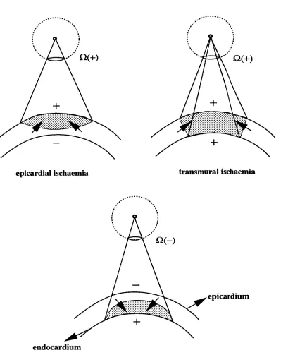
Solid Angle (S2)

Double layer ...

•

(13 = (p/47ca) *

• A

Figure 2.5: Illustration of solid angle theory. The potential at point A (4)) produced by

the uniform double layer with the strength p in an infinite medium is proportional to the

double layer strength and the solid angle (C2) of point A subtended by the double layer

boundary. (From Hans and Melcher [36]).

further assumed that the potential difference at the boundary was proportional to the double-layer strength, i.e.

1

41) =

47ro- = VD -47rCl (2.9)

where p denotes the current dipole density and VD the potential jump over the double layer. The potential distribution at the activation boundary showed an S-shaped curve rather than an abrupt jump noted by Solomon and Selvester [58]. The following function was used to describe the source potential distribution by van Oosterom [33].

8(x) = ₍ (2.10)

x2 + 1472)1/2

where W is a measure of the width of the source distribution (Figure 2.6). Consequently, the potential 0(x) at the wavefront due to the local sources could be given by

(31)

_

-

_

-

_

-

S(x), W = 0.1 — _

-

-1 -0.8 -0.6 -0.4 -0.2 0 0.2 0.4 0.6 0.8 1

Figure 2.6: The shape of the potential distribution over the activation boundary used by

van Oosteroin [31].

It was assumed that VD

=

40mV during depolarisation and W = 0.8mm following the recordings with multi-terminal intramural electrodes in dogs [59, 33]. A number of triangles were used to approximate the activation wavefront at each time instant considered. The positions of these triangles were based on the data of Durrer et

al. [49]. A triangulated representation of the torso surface was used. Plonsey [30]

calculated the body surface potential using integral equation formulation, which calculated the potentials at the torso surface from the known strength of a uniform double layer in a homogeneous and bounded medium. The simulated body surface potentials for 11 time instants at 5ms intervals during depolarisation were in a similar order of magnitude to those recorded in healthy subjects.

Solid angle theory was widely used to study ST segment changes in myocardial ischaemia by Holland's group [60, 61] in which the source at the ischaemic boundary was represented by the difference in the action potential between the normal and ischaemic cells (64,„).

47r (2.12)

The details of this approach will be discussed in the next chapter.

(32)

2.4.5 Bidomain model

The bidomain model, in which myocardium is represented by two superimposed but distinct continuous domains, intracellular and extracellular, separated everywhere by the cell membrane, was first derived in the late 1970s by Tung [62] and Miller and Geselowitz [34]. The model describes the average behaviour of the bioelectric fields of cardiac muscle over distances that are large compared with the size of a single cell. If

I

is the current density, (1) the potential and a the conductivity, then

=

(2.13)

:le = —7eV0e

(2.14)

where the subscripts i and e represent intracellular and extracellular spaces respec-tively. The charges moving from one domain to the other must cross the membrane and hence represent membrane current per unit volume (/„,). The fundamental equation describing the potentials in cardiac tissue is the conservation of the cur-rent [62]. Mathematically

V • ai V(Di = Im (2.15)

V • aeVcI), = (2.16)

v • (ii +

fe) = o

(2.17)

By definition, the transmembrane potential

Om = —

Oe

(2.18)

Combining these equations yields equations for both intracellular and extracellular potentials:

V • a-VO, = —V' • cr2 V(1),7, (2.19)

V aV(Di = V • o-eVOm (2.20)

(33)

The bidomain model has been applied extensively in cardiac electrophysiology. It

has been used to compute intracellular and extracellular potentials when the action

potential is known [63, 64, 65] and to calculate the transmembrane potential induced

in passive tissue in response to applied currents [66, 67, 68, 69].

Miller and Geselowitz [34] applied the bidomain model in a slightly different context.

Combining equations (2.15) and (2.16) gives

V • aV i = — • creVA), (2.21)

which is reduced to

v% = —(

5i

kie)v

2

(Di =

lv • ,r

i

cie (2.22)

when the two domains are assumed to be isotropic. From equation (2.13), the

intracellular current density (.4) can be interpreted as the current dipole moment

per unit volume, and is proportional to the spatial gradient of the intracellular

potential distribution. It is evident from equation (2.22) that the potential (I), can

be considered to arise from a cardiac current generator which can be represented by

the intracellular current density (ii).

Miller and Geselowitz [34] represented the ventricular anatomy with a 3-D array

of approximately 4000 points, which was assumed to be located in a homogeneous

volume conductor with the shape of an adult torso. An assumed action potential

shape was used with a ventricular gradient, in which depolarisation was modelled

by a step change from the resting value of -90mV to 10mV at the activation time

and repolarisation by a series of six linear segments (Figure 2.7). Isochrones were

specified at each point on the basis of the human heart data of Durrer et al. [49], and

the simulated intracellular potential at each point in the heart model was calculated

using the assigned activation times and action potential data. The current dipole

at each point was approximated by the discrete difference of the potentials at its

six nearest neighbours. The moments of 23 dipoles were obtained by summing the

moments of the dipoles at all the points within the corresponding regions of the

heart model. Then the potentials on the surface of the torso were calculated from

the set of 23 dipoles using the transfer coefficient previously obtained by Cuffin and

(34)

10 —

o

mV

—90

0 100 200 300

(msec)

Figure 2.7: The cellular action potential model with the longest and shortest action

po-tentials used in the normal heart simulation. (From Miller and Geselowitz [32]).

The simulation results from Miller and Geselowitz [34, 70] appeared to provide an excellent simulation of the body surface ECG for the normal and abnormal hearts. However, it is not clear how the intracellular potentials were simulated with the known transmembrane potential and activation times. It is extremely difficult to measure the spatial distribution of intracellular potentials. Also, endocardial and epicardial potentials were not addressed in the study, and thoracic inhomogeneity and myocardial anisotropy were ignored in the model.

In another model [71], the ventricles together with bundle branches and Purkinje fibres, were composed of approximately 50000 cubic cell units. The action potential waveforms with different durations in the plateau phase were assigned to the indi-vidual cells. The heart model was mounted in a homogeneous human torso model with a conductivity of at . The dipole generated at each cell unit was calculated as

f(r, t) = t) (2.23)

where (1.,„(r, t) denotes the action potential at time t of the cell located at r, and am

(35)

the extracellular potential (D e satisfies Poisson's equation:

V • atV(De = V • f (2.24)

The potentials were calculated by the boundary element method in which Poisson's equation with homogeneous Neumann's boundary conditions on the torso surface was modified to Laplace's equation with inhomogeneous boundary conditions. The resulting ECG, VCG, and body surface potential maps (BSPM) were within the expected range of the clinical observation.

A similar concept was employed in the "SI" (spatial intracellular potential) model of Spach et al. [72]. It was assumed that a network of cells could be treated as one large cell so that the net membrane current could still be determined by the core model of Plonsey [30], that is, the membrane current could be approximated by the second spatial derivative of the intracellular potential (D i evaluated along the fibre axis z.

Jm(t, z) aza

a2

)2(t ,

2 az2 (2.25)

The extracellular potentials could be calculated from the membrane current, based on Green's theorem [30]. The measured intracellular potentials were used to de-termine the extracellular potentials in their study. In separate experiments, this model successfully predicted the extracellular potentials surrounding a single Purk-inje strand [72] and the normal epicardial ST-T potentials resulting from ectopic beats in dogs [73]. However, only a simplified ventricle geometry was used in the simulations.

2.5 Anisotropy

(36)

variability in the measured conductivity values. Firstly, whether intracellular or ex-tracellular space has a higher conductivity has not yet been determined. The ratio of the measured extracellular to intracellular conductivities varied from 0.28 [75] to 1.2 [78]. Secondly, the ratio of the measured longitudinal to transverse conductivities in either space varied greatly. For instance, the ratio for the intracellular domain ranged from 5.77 [79] to 10.57 [80]. Despite this inconsistency, the longitudinal conductivity is surely much greater than the transverse conductivity. Therefore (D i and (De depend not only on the value of the conductivity, but also on the direction relative to the fibre axis.

The uniform double layer model is not an accurate description of the myocardial activation because it does not take anisotropy into account [81, 79]. The bidomain model can take anisotropy into consideration. If a is assumed to be anisotropic, equation (2.19) no longer possesses a simple solution. However, if the myocardial anisotropy (a) is assumed to be constant, then Poisson's equation still holds, and the mathematics remains tractable. In this case, the source term which is associated with ai , will depend on whether the direction is parallel or transverse to the fibre axis. There are two simplified approaches to study the effects of anisotropy on the potential distribution.

2.5.1 Axial model

(37)

times as great in the longitudinal direction.

2.5.2 Oblique dipole layer

The assumption of purely axial orientation of cellular dipoles is an improvement over the uniform dipole theory [82]. However, as pointed out by Roberts et al.

[81], the axial model probably predicted too strongly a dependence of the wavefront voltage on the fibre orientation. An oblique dipole model was suggested by Colli-Franzone et al. [83], which took both axial and transverse dipoles into account. The numerical simulations were carried out in an isotropic homogeneous medium with the shape of a cylinder (15cm in height and 23cm in diameter) as used in their experiments. The wavefront shape was assumed to be semi-ellipsoidal when the endocardium was paced. They found that the calculated potentials from the oblique dipole with longitudinal dipole moment m i and transverse moment mt matched the measurements of the paced dog hearts in the volume conductor when the ratio mi/rnt was between 15 and 30. They also showed that the axial component of the potential field played a dominant role with respect to the normal component.

Roberts and Scher [79] solved equation (2.19) in the bidomain model analytically for a depolarisation in an infinite homogeneous medium with a simplified wavefront shape. The potentials were calculated by a surface integral where the wavefront was represented by a wavefront voltage, which was assumed to be a step function

(AV=100mV). The extracellular potential in the wavefront was taken as

Vol = AV (ait I al) (2.26)

Vot = (aid at) (2.27)

(38)

2.5.3 Full anisotropic model

Myocardial anisotropy affects not only the source but also the property of the myocardial part of the volume conductor (equation 2.19). The overall effects of anisotropy on the ECGs have been widely studied with this approach [84, 35]; how-ever, the detailed analysis of the equation has been performed only on simplified two or three dimensional geometries.

A study carried out on 2D anisotropic tissue due to a circular-shaped wavefront using the bidomain model by Sepulveda and Wikswo [85], showed that simple depo-larisation wavefronts produced complex current distribution as predicted by Plonsey and Barr [86].

The study of the effect of anisotropy by Colli-Franzone et al. [65] was carried out on a myocardial slab during paced beats using the bidomain model. The results were consistent with the predictions of the oblique dipole layer model [83]. It was found that the epicardial and endocardial potential maps provided information on the pacing site and depth, and on subsequent intramural propagation, by reflecting the clockwise or counterclockwise rotation of the deep positivity.

In Pollard and Burgess' study [35], a model of a 3D block was comprised of net-works of microscopic elements arranged into rectangular parallelepipeds in which epicardial stimulation was applied. They found that the rotation of fibre axes ac-celerated epicardial activation distant from the stimulus site. The inhomogeneous conductivity caused regional acceleration and deceleration spread.

(39)

between the isotropic and anisotropic myocardium.

(40)

Chapter 3 Literature review

3.1 Introduction

This chapter provides information on myocardial ischaemia, including its

occur-rence, the transmembrane potential of ischaemic cells, ischaemic boundaries, and its

associated ST segment shift. It mainly covers mathematical models and the

experi-mental and clinical observations of ST changes in ischaemia. Finally, the advantages

and disadvantages of the models are discussed in terms of being able to explain the

observations.

3.2 Myocardial ischaemia

Myocardial ischaemia occurs when coronary artery blood flow is insufficient to meet

the myocardial metabolic requirements. This insufficiency of blood supply can result

from either artery restrictions such as induced occlusion in experiments and coronary

artery occlusion in patients, or greater demand from exercise testing in the presence

of partial narrowing. Ischaemia affects myocardial cells by inducing ionic, metabolic,

electrical and mechanical changes. The electrical changes are basically those of

changed transmembrane potential, which affect injury current, ECG, recovery of

excitability and electrical conduction. This review focuses only on the changes in

(41)

CHAPTER 3. LITERATURE REVIEW 29

mv

10- £

0 -

normal cells ischaemic cells

—60

—90 4

Figure 3.1: Waveform of the action potential of normal cells (solid line) and ischaemic

cells (dotted line). Normal cells have a resting potential of -90mV and ischaemic cells

-60mV.

the transmembrane potential, the injury current associated with ischaemia and ST segment shifts in ischaemia.

3.2.1 Transmembrane potential of ischaemic cells

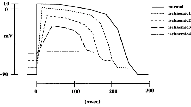
It is well documented that ischaemia causes changes in the transmembrane potential of the affected cells [90, 91, 92, 8, 93]. The typical changes include a decrease of the resting membrane potential, a shorter duration of the action potential and a decrease of amplitude of the action potential. The times of onset and up-stroke of the action potential are also changed (Figure 3.1).

In 1960, Samson and Scher [90] observed that the plateau of the intracellular action potential was of a shorter duration after 4 minutes of

Coronary artery ligation in

(42)

CHAPTER 3. LITERATURE REVIEW

Other intracellular recordings [91] showed a substantial loss in the resting membrane potential, small changes in the duration and amplitude of phase 2 and in the slope of phase 3. Similar results were obtained in porcine hearts [8, 94]. Following the LAD occlusion in pigs, the first change was a decrease in the resting transmembrane potential; after a further 3 minutes, the action potentials were shortened and their amplitude reduced; finally, the ischaemic cells became totally unresponsive at a resting potential of about -60 to -65mV within 7-10 minutes of occlusion [8].

The degree of changes in the transmembrane potential varies with the time course of ischaemia. The transmembrane potential of ischaemic cells can vary from "near normal" to having a very small amplitude, depending on the location and duration of ischaemia [8].

3.2.2 ST segment shift

(43)

action potential between normal and ischaemic cells produces a current source in the ischaemic side and a current sink in the normal side in the extracellular space. Electrical potential caused by this current during phase 2 is called the true ST seg-ment shift. Thus ST elevation is registered in the ischaemic area and ST depression in the normal area. In a conventional AC coupled ECG recorder, TQ change and ST change can not be differentiated and the recorded ST change is a combination of both. Therefore both TQ depression and ST elevation are shown as ST eleva-tion, while TQ elevation and ST depression are contributors to the recorded ST depression. The time course and the predominance of ST or TQ segment changes in ischaemia have not yet been settled [90, 91, 92, 8, 96], but this is beyond the scope of this review.

ST elevation and ST depression can appear depending on the ischaemic location and the recording position. For example, ST elevation is registered over the ischaemic region on the epicardium during transmural ischaemia [21]. Meanwhile ST depres-sion appears over the non-ischaemic region on the epicardium. In the same study, however, ST elevation is registered over the ischaemic region on the endocardium while ST depression appears on the epicardium during subendocardial ischaemia.

3.2.3 Ischaemic region and boundary

(44)

ischaemic border normal ischaemie side

■

OmV

—30mV

extracellular

ischaemic border normal

(b)

—60mV —90mV

P2

— normal cell • • ischaemic cells

2

Phase 4 (P4)

extracellular

(a)

CHAPTER 3. LITERATURE REVIEW

32 Figure 3.2:

Illustration of cellular current and TQ/ST changes produced in the ischaemic

boundary. In diagram (a), the top figure shows the action potentials of normal cells (solid

line) and ischaemic cells (dotted line), the middle shows normal ECG (solid line) and

ischaemic ECG (dotted line) in the ischaemic side, and the bottom shows normal ECG

(solid line) and ischaemic ECG (dotted line) in the normal side. Diagram (b) shows

the polarity of TQ/ST changes during phase

4 (P4)

and phase 2 (P2) of the AP. Sign

f

indicates elevation and _4. depression. Signs (+) and (-) indicate the source polarity. During the P4, the resting potential of normal cells is -90mV and ischaemic cells -60m V.

(45)

are referred to as ischaemia of a large region. Both LAD and LCX have their own branches, and ligation of such a branch artery results in ischaemia of a small region. A study carried out in Dorset sheep [98] showed that the LAD had its first branch originating high on the anterior wall of the left ventricle, and that the second branch had a variable site of origin at the middle-LAD distributing over the lower anterior wall and apex. The LCX extended around to the posterior wall to give 2-3 marginal branches and a short posterior descending artery with septal branches.

The ischaemic boundary is another factor to influence the current sources derived from ischaemia. The existence and width of ischaemic gradients at the ischaemic boundaries are still debatable [99]. Many investigators have studied the myocardial blood flow [100, 101, 102], metabolic changes [103, 101] and electrophysiological changes [104, 105, 103] in samples from the lateral edges of the ischaemic regions. Some maintained that the transitional zone is a border zone of intermediate injury tissue [104, 106, 105]. But most agree that the transition from non-ischaemic to ischaemic tissues is sharp [100, 101, 102, 97].

Reimer and Jennings [100] suggested that the zone of intermediate reduction in blood flow between non-ischaemic and ischaemic regions in dogs occurs in a 1-2mm section because of interdigitation of ischaemic and normal cells. Studies of blood flow after acute coronary artery occlusion in dogs showed that the transition of an intermediate reduction in blood flow was limited to a narrow rim of myocardium of 3mm or less in width immediately inside the ischaemic region, and that the intermediate reduction in blood flow at the border resulted from an admixture of normal and ischaemic myocardium [102]. Euler and co-workers [97] observed that ligation of the LCX produced a sharp boundary between perfused and non-perfused tissues in the ovine heart. An electrophysiological, metabolic and histochemical study of the ischaemic boundary in the pig heart indicated that cells with nearly normal transmembrane potential were in close proximity to unresponsive cells with low resting potentials, suggesting that the ischaemic border was composed of interdigitating normal and ischaemic zones sharply demarcated from each other [103].

(46)

is less well established. However, it is well known that the subendocardial segment is more frequently and more severely affected than the epicardial segment following coronary artery ligation [107]. Some studies of blood flow have shown that there is a gradual change in blood flow from the epicardium to the endocardium for partial thickness ischaemia [100, 108]. This suggests that there may be a border zone of intermediate injury between the ischaemic and normal regions in the transmural wall.

3.3 ST segment models during ischaemia

The ST segment is a part of the ECG. Like the QRS complex (Section 2.3.2), simulation of the ST segment potential includes two aspects: the cardiac current source and the volume conductor. Here four equivalent injury current generators and one cellular source description are discussed, including their potential distributions in various volume conductors.

3.3.1 Dipole theory

(47)

depression while the cavity and opposing wall should yield ST elevation [111, 112].

For transmural ischaemia in the anterior wall, ST elevation appeared in the anterior,

posterior and cavity leads.

The dipole theory can be used to approximate far field such as body surface

poten-tials. Studies of body surface mapping in transmural ischaemia or infarction showed

that ST elevation appeared in the ischaemic region while ST depression appeared in

the opposite site [113, 114 However, the maximum ST elevation on the epicardium

does not necessarily occur over the centre of ischaemia [114]. Localised ST segment

changes on the epicardium do not correspond to changes on the thoracic surface

[114]. Although the dipole theory provides the basic information on ST changes on

the body surface in transmural ischaemia, it does not work for ST depression in

subendocardial ischaemia [4, 21].

3.3.2 Multiple dipoles

A multiple-dipole model was used by Thiry and co-workers [48, 1151, with the

ven-tricles being divided into 11 regions and each region being characterised by a dipole

at the region's centre. The dipole had a fixed position and direction and a variable

strength. They modelled acute ischaemia by reducing the amplitude of the action

potential by

20%

in one cell of a contiguous pair while keeping the other unchanged

(48)

dial ischaemia, although twice as much tissue volume was ischaemic in the epicardial case. The reduction in transmembrane potential amplitude was proportional to the volume of ischaemic tissue; the contiguity effect produced on the ischaemic bound-ary was an area effect. They concluded that the ST change was not a quantitative measure of the ischaemic volume but a measure of the cross-sectional area of such tissue normal to the direction of signal propagation. In this approach, however, other factors such as the realistic ischaemic boundary and the volume conductor were not taken into account.

As will be discussed in Section 3.3.5.2, Miller and Geselowitz [70] simulated is-chaemia with 23 dipoles calculated from the bidomain model.

3.3.3 Multipole

Another alternative to the dipole model is to represent the current generator with a dipole having higher order moments. Mirvis et al. [113] determined the equiva-lent generator properties of acute transmural ischaemia inversely from the measured potentials on a sphere (6.25cm) of conductive solution in which an isolated rabbit heart was placed. The 32 ECG signals on the sphere surface were processed to quantify the potentials during ST segment attributable to a central dipole, a four-element multipole (dipole, quadrupole, octopole, hexadecapole) and a single moving dipole during ST segment. Fifteen minutes following the LAD ligation, 74%, 98% and 96% of summed square potential recorded 10 msec into the ST segment could be accounted for by a central dipole, a four-element multipole dipole and a single moving dipole model respectively. Furthermore, during the ST segment, the mo-ment of the single moving dipole correlated directly with the area of the epicardial lesion (r=0.82). The surface potential maps uniformly demonstrated a single ST elevation maximum which was aligned with the ischaemic lesion, with an intensity proportional to the computed dipole moment and the epicardial size. Thus the four-element central multipole dipole and the single moving dipole models provide a quantitatively accurate description of the experimental data.