A spectrum of compromise aggregation operators for multi attribute decision making

(1)

A spectrum of compromise aggregation operators for multi-attribute

decision making

Xudong Luo

∗

, Nicholas R. Jennings

School of Electronics and Computer Science, The University of Southampton, Highfield, Southampton SO17 1BJ, United Kingdom

Received 4 May 2006; received in revised form 8 November 2006; accepted 10 November 2006

Abstract

In many decision making problems, a number of independent attributes or criteria are often used to individually rate an alternative from an agent’s local perspective and then these individual ratings are combined to produce an overall assessment. Now, in cases where these individual ratings are not in complete agreement, the overall rating should be somewhere in between the extremes that have been suggested. However, there are many possibilities for the aggregated value. Given this, this paper systematically explores the space of possible compromise operatorsfor such multi-attribute decision making problems. Specifically, we axiomatically identify the complete spectrum of such operators in terms of the properties they should satisfy, and show the main ones that are widely used—namely averaging operators, uninorms and nullnorms—represent only three of the nine types we identify. For each type, we then go onto analyse their properties and discuss how specific instances can actually be developed. Finally, to illustrate the richness of our framework, we show how a wide range of operators are needed to model the various attitudes that a user may have for aggregation in a given scenario (bidding in multi-attribute auctions).

Keywords:Aggregation operator; Uninorm; Nullnorm; Risk; Multi-attribute decision making; Multi-attribute auction

1. Introduction

Decision making is a central concern in the area of artificial intelligence and it is thus an essential component of many intelligent systems. For this reason, many decision making models have been developed (such as knowledge-based reasoning [5,47], case-knowledge-based reasoning [37], neural networks [20], and constraint satisfaction techniques [44, 48]). Now, in many cases, the decision making that is performed needs to consider multiple criteria or attributes. In such cases, the decision making agent is faced with a set of decision alternatives and the ratings per alternative per criterion (that indicate the degree of satisfaction of the criteria by the alternative) which then have to be fused together in order to produce an overall rating. This fusion process is carried out by some form ofaggregation operation[9,60]. In most cases, this operation is some form of weighted arithmetic mean [19]. Now, this works well in situations in which any differences are viewed as being in conflict because the operator reflects a form of compromise behaviour among the various criteria. However, when these conditions do not hold, arithmetic mean is a poor choice. Thus, in

* _{Corresponding author.}

(2)

general, the type of aggregation used should reflect the user’s individual choice of behaviour among criteria. Given this observation, we seek to develop a comprehensive set of possibilities for this task and to do so we turn to fuzzy set theory (see [17] for a view on the importance and impact of this line of research on the general area of artificial intelligence). Our motivation for this choice can be summarised by the following insight [3]:

“In fuzzy set theory, membership functions of fuzzy sets play the role similar to utility functions—the role of de-grees of preference. Many authors, including Zadeh himself, refer to membership functions as ‘a kind of utility functions’. The equivalence of utility and membership functions extends from semantical to syntactical level. Al-though this is not the only possible interpretation of membership functions, it allows one to formulate and solve problems of multiple criteria decision making using the formalism of fuzzy set theory.”

In more detail, in fuzzy set theory, the two most widely used aggregation operators are t-norms and t-conorms that model “AND” and “OR” fuzzy connectives [14,23,32], respectively. However, their main limitation in terms of aggregation is that the ensuing result is not a compromise between low and high ratings, which, in many cases, is a serious shortcoming [64,65]. To rectify this, alternative aggregation operators have been proposed as a means of obtaining such a compromise (e.g., averaging operators [1,16,24,26,35], uninorm operators with a neutral element [52,62], and nullnorms (or t-operators) [8,50,51]). Furthermore, the general cases of the two extremes (minimum and maximum) are t-norm and t-conorm and thus aggregation operators for obtaining a compromise between a pair of t-norms and t-conorms have also been developed (e.g.,γ-operators [64], exponential compensatory operators [57], and convex-linear compensatory operators [39,57]). However, in all of this work, there is no common, systematic framework that enables the complete space of possibilities to be mapped out. This means that the sometimes subtle differences between all these operators are not always readily apparent and that whole families of possibilities may be missed out. This paper seek to rectify this shortcoming by systematically mapping out the space of possibilities.

By way of illustration, consider the following applications of these operators in a variety of intelligent systems.

Firstly, they have been employed in a number of agent-based systems. For example, in an agent-based automated negotiation system that we have developed for business to consumer e-commerce, such an operator is employed to aggregate the satisfaction degree for a product and its purchasing conditions in order to decide whether or not it is acceptable [43]. In this case, when a customer does not like the product sufficiently much on its own, but the purchasing conditions (e.g., finance deal and delivery time) are very attractive, the aggregated acceptance degree for the goods is somewhere in-between the individual ratings, and thus the customer may decide to make the purchase if the overall deal is sufficiently attractive. Similarly, in an agent-based meeting scheduling system, we use an operator to aggregate all the participating agents’ individual ratings for a possible common time slot into an overall rating for that slot [45]. Thus, in this case, when some agents are inclined to reject a meeting time proposal and others are inclined to accept it, the aggregated rating for the proposal is somewhere in-between their individual ratings. Secondly, aggregation operators have been employed in expert systems. For example, in distributed expert systems, such operators have been exploited to synthesise different expert systems’ uncertainties (ratings) for a particular conclusion [63]. Thus, when a conclusion is convincing for some expert systems, but not for others, the aggregated uncertainty for the conclusion is in-between the individual uncertainties. Similarly, in stand-alone rule-based systems, such operators have been used to aggregate uncertainties (ratings) of the same proposition that are drawn in parallel from different sources [2,46, 56]. Thus, when uncertainty from some sources do not support the proposition, but the ones from the others do, its aggregated uncertainty is in-between the individual uncertainties.Finally, aggregation operators have been employed in many other decision making systems. For example, in fuzzy rule systems, such operators are used to aggregate the output of individual rules to obtain the overall system output [61]; in specific kinds of artificial neural networks where uncertainty handling is necessary, they are used as a threshold function [56]; and in video query systems, they are used to aggregate matching degrees of video attributes to a global matching degree [13].

(3)

situation becomes even more complex. In particular, even if we assume that the result of aggregating two conflicting ratings (i.e., one higher than the threshold and one lower) is in-between the two, there are still a number of different ways (as discussed above) to aggregate two positive ratings or two negative ones.

Such issues are important in a number of contexts. On the one hand, cognitive psychology has showed that the human brain is very efficient at processing bipolar (negative and positive) information [6,7,54]. It is believed that this is so because of the way in which a large part of this expertise is acquired, and also likely to be a result of the cognitive evolution of species. One the other hand, whenever we want decision making agents to act on behalf of users, the agent must be capable of reflecting their individual nuances, preferences and attitudes to risk [10,40–42]. In both of these cases, flexible aggregation is an integral component of this.

Despite its importance, the issues associated with users’ attitudes in the aggregation of attributes’ ratings, distin-guished as positive and negative categories, have received comparatively little attention to date. In fact, in [4], the bipolar view is taken in modelling preferences. However, in our work it is used for modelling the scales of attributes’ ratings. More importantly, the focus of [4] is modelling negative and positive preferences separately in the framework of possibility theory, and so such preferences are aggregated simply using fixed operators. This leaves the issue of exploring the whole space of all possible operators undiscussed. At this point, it is similar for the other works of bipolar preference representation, such as Cumulative Prospect theory [58], multi-criteria decision making [25], and Artificial Intelligence work that is oriented towards qualitative decision [36,59].

Given this background, our aim in this paper is to impose greater structure on the problem by exploring all the possible combinations of these attitudes in compromise aggregation. More precisely, we advance the state of the art by distilling a number of properties that are common to various types of compromise operators (including averaging operators, uninorms and nullnorms) and also identifying several new types of compromise operators in order to model the various attitudes that users may have when aggregating non-conflicting ratings. We then go onto analyse the properties of all aggregation outcomes and devise some construction methods that can be used to develop specific instances of these operators for particular contexts. Finally, in order to illustrate that the richness of these operators is necessary in practice, we examine them in the context of a particular application of rating bids in multi-attribute auctions.

The rest of the paper is organised as follows. By analysing two existing kinds of compromise operator and general aggregation operators, Section 2 introduces the concept of general compromise operators. Section 3 further identifies a number of new types of compromise operators and discusses how they reflect users’ attitudes to risk in aggregation. Sections 4–6 discuss the properties of the various operators and the methods for constructing them. Section 7 illustrates the application of compromise operators in a multi-attribute auction scenario. The last section summarises our main contributions and sheds light on future avenues of research.

2. Generalised compromise operators

This section first analyses the fundamental concepts of two kinds of existing compromise operators [1,62] and of general aggregation operators [34]. Based on this analysis, we then introduce the concept of a general compromise operator that, in turn, induces several new types of compromise operator.

2.1. Analysis

The first type of existing compromise operators that we consider are uninorm compromise operators. These are a special case of uninorm operators [52,62]:

Definition 1.A binary operatorU: [0,1] × [0,1] → [0,1]is auninormif:

(1.1) monotonicity:∀a1, a₁, a2, a₂ ∈ [0,1],a1a₁, a2a₂ ⇒U(a1, a2)U(a₁, a₂);

(1.2) associativity:∀a1, a2, a3∈ [0,1],U(U(a1, a2), a3)=U(a1,U(a2, a3));

(1.3) commutativity:∀a1, a2∈ [0,1],U(a1, a2)=U(a2, a1); and

(4)

In particular, when the neutral elementτ is 1, 0, and between 1 and 0, respectively, the uninorm operator is called a

t-norm(denoted asT), at-conorm(denoted asS), and auninorm compromise operator(denoted asUτ).

Example 1.The following is a uninorm compromise operator [31]:

U(P )_τ (a1, a2)=

(1−τ )a1a2

(1−τ )a1a2+τ (1−a1)(1−a2)

, (1)

whereτ ∈(0,1)is its neutral element.

The lemma below gives a property of uninorm compromise operators [62].

Lemma 1.

∀τ₁+, τ₂+∈(τ,1], Uτ(τ1+, τ2+)max{τ1+, τ2+}, (2)

∀τ₁−, τ₂−∈ [0, τ ), Uτ(τ1−, τ2−)min{τ1−, τ2−}, (3)

∀τ−[0, τ ), τ+∈(τ,1], τ−Uτ(τ−, τ+)τ+. (4)

Proof. According to the monotonicity and neutral element property of uninorm operators, ∀τ₁+, τ₂+, τ+∈(τ,1], τ₁−, τ₂−, τ−∈ [0, τ ), we have:

Uτ(τ₁+, τ₂+)Uτ(τ₁+, τ )=τ₁+ Uτ(τ₁+, τ₂+)Uτ(τ, τ₂+)=τ₂+

⇒Uτ(τ1+, τ2+)max{τ1+, τ2+};

Uτ(τ₁−, τ₂−)Uτ(τ₁−, τ )=τ₁− Uτ(τ₁−, τ₂−)Uτ(τ, τ₂−)=τ₂−

⇒Uτ(τ₁−, τ₂−)min{τ₁−, τ₂−};

Uτ(τ−, τ+)Uτ(τ−, τ )=τ− Uτ(τ−, τ+)Uτ(τ, τ+)=τ+

⇒τ−Uτ(τ−, τ+)τ+. 2

According to this lemma, we can regard the neutral element of a uninorm compromise operator as a threshold: if a rating is greater than the threshold it is regarded aspositive, otherwise it is regarded asnegative. Thus, in Lemma 1, property (2) reflects the intuition that when two ratings are both positive, they enhance the effect of each other in aggre-gation; property (3) that when two ratings are both negative, they weaken each other in aggreaggre-gation; and property (4) that when two ratings are in conflict, a compromise result of aggregation is obtained.

Another important property of uninorm operators that will be used later is:

Lemma 2.

(1) Monotonicity:∀a1, a1, . . . , an, an∈ [0,1],

a1a1, . . . , anan ⇒Uτ(a1, . . . , an)Uτ(a1, . . . , an); (5)

(2) Symmetry:∀a1, . . . , an∈ [0,1],

{p1, . . . , pn} = {1, . . . , n} ⇒Uτ(a1, . . . , an)=Uτ(ap1, . . . , apn). (6)

Property (5) in the above lemma means that operatorUτis monotonically non-decreasing, and property (6) that the result of aggregation using the operator is independent of the order of aggregation (i.e., it is symmetric). For example, we have:

Example 2.From the uninorm (1) we can derive the following symmetric formula:

U(P )_τ (a1, . . . , an)=

1

1+₁₋τ_τn−1n_i₌₁1−ai

ai

(5)

A number of important properties of t-norms and t-conorms, which will be used later, are as follows:

Lemma 3.∀a1, . . . , an∈ [0,1],

T(a1, . . . , an)min{a1, . . . , an}max{a1, . . . , an}S(a1, . . . , an); (8)

T(0, . . . ,0)=0; (9)

S(1, . . . ,1)=1. (10)

The second type of existing compromise operators that we consider are averaging operators, these are defined in following way [1]:

Definition 2.A mappingM:_n_∈N[0,1]n→ [0,1]is anaveraging operatorif:

(2.1) idempotency:∀a∈ [0,1],M(a, . . . , a)=a;

(2.2) monotonicity:∀a1, a₁, . . . , an, an ∈ [0,1],a1a₁, . . . , anan ⇒M(a1, . . . , an)M(a₁, . . . , an); and (2.3) symmetry:∀a1, . . . , an∈ [0,1],{p1, . . . , pn} = {1, . . . , n} ⇒M(a1, . . . , an)=M(ap1, . . . , apn). Example 3.The arithmetical mean is a typical averaging operator:

MA(a1, . . . , an)=

a1+ · · · +an

n . (11)

The lemma below gives an important property of averaging operators.

Lemma 4.∀a1, . . . , an∈ [0,1],

min{a1, . . . , an}M(a1, . . . , an)max{a1, . . . , an}. (12)

This lemma means that any two different ratings are always regarded as being in conflict and so it is always the case that a compromise result is obtained by an averaging operatorM. Comparing Lemma 4 with Lemma 1, we can see that for a compromise aggregation operator, property (4) is essential, but properties (2) and (3) could be relaxed and replaced by others (at least in an averaging operator M they can be replaced by min{a1, a2}M(a1, a2)

max{a1, a2}). Accordingly, we cangeneralisethe concept of a compromise operator such that it can cover uninorm

compromise operators and averaging operators (or so called averaging compromise operators) as its special cases. That is, generalised compromise operators are those that exhibit properties (4) and (12) (but not necessarily (2) and (3)). Then, furthermore, since the generalised compromise operators are aggregation operators, they should satisfy the properties of general aggregation operators [34]:

Definition 3.A mappingA:_n_∈N[0,1]n→ [0,1]is ageneral aggregation operatorif:

(3.1) boundary conditions:A(0, . . . ,0)=0 andA(1, . . . ,1)=1;

(3.2) monotonicity:∀a1, a₁, . . . , an, an ∈ [0,1],a1a₁, . . . , anan ⇒A(a1, . . . , an)A(a₁, . . . , an); (3.3) symmetry:∀a1, . . . , an∈ [0,1],{p1, . . . , pn} = {1, . . . , n} ⇒A(a1, . . . , an)=A(ap1, . . . , apn).

Clearly, uninorm compromise operators and averaging operators are special cases of the general aggregation oper-ator. Of course, t-norms and t-conorms are also special cases since they are special cases of a uninorm.

Based on the above analysis, the next subsection will introduce our concept of generalised compromise operators.

2.2. Generalised compromise operators

(6)

form of trade-off between the best and the worst of the individual ratings. Second, all compromise operators should satisfy the properties of general aggregation operators. Based on these two points, we define the concept of a general compromise operator as follows:

Definition 4.A general aggregation operator is ageneral compromise operator, denoted asCτ, with respect toτ ∈ (0,1)if∀τ₁−, . . . , τ_k−∈ [0, τ ), τ₁+, . . . , τ_l+∈(τ,1](k, l1, k+l=n),

min{τ₁−, . . . , τ_k−}Cτ(τ₁−, . . . , τ_k−, τ₁+, . . . , τ_l+)max{τ₁+, . . . , τ_l+}. (13) A general compromise operatorCτis uninorm-like1if∀τ₁−, . . . , τ_l−∈ [0, τ ),τ₁+, . . . , τ_k+∈(τ,1](k, l1, k+l=n),

Cτ(τ₁−, . . . , τ_l−, τ, τ₁+, . . . , τ_k+)=Cτ(τ₁−, . . . , τ_l−, τ₁+, . . . , τ_k+); otherwise it is averaging-like.2

In the above definition, (13) reflects properties (4) and (12).3Moreover, in the following section, we will see clearly that for general compromise operators, properties (2) and (3) can be replaced by other properties (in order to reflect the decision makers’ attitudes to risk in aggregating non-conflicting ratings). In addition, from the proof of Lemma 1, we can see that the neutral element of a uninorm plays a key role in ensuring it satisfies (13). However, it can be relaxed a little and (13) can still be satisfied. Formally, we have:

Theorem 1.A general aggregation operatorAτ:

n∈N[0,1]n→ [0,1]is ageneral compromise operatorwith respect

toτ ∈(0,1)if∀τ₁−, . . . , τ_k−∈ [0, τ ),τ₁+, . . . , τ_l+∈(τ,1],

Aτ(τ₁−, . . . , τ_k−, τ )Aτ(τ₁−, . . . , τ_k−, τ₁+,· · ·, τ_l+)Aτ(τ₁+, . . . , τ_l+, τ ), (14)

Aτ(τ₁−, . . . , τ_k−, τ )min{τ₁−, . . . , τ_k−}, (15)

Aτ(τ₁+, . . . , τ_l+, τ )max{τ₁+, . . . , τ_l+}. (16)

Proof. Clearly, from (14)–(16) we can derive (13). 2

In the above theorem, letl=1 andk=1 then (15) and (16) become:

Aτ(τ₁−, τ )τ₁−, (17)

Aτ(τ₁+, τ )τ₁+. (18)

Thus, the above two can be seen to be a generalisation of the concept of a neutral element of a uninorm (and if we let τ=1 or 0 in (17) and (18), we can get the corresponding generalisations of t-norms and t-conorms).4

Now, we turn to the issue of confirming that our general compromise operators can cover the existing compromise operators: uninorms compromise operators, averaging operators and nullnorms. First, we have the following obvious theorem:

Theorem 2.Uninorm compromise operators and averaging operators are special cases of general compromise oper-ators.

1 _{That is, like a uninorm operator, it has a unit element}_τ_. 2 _{That is, like an averaging operator, it has no any unit element.}

3 _{However, we cannot replace the boundary condition of general aggregation operators by:}

Cτ(a1, . . . , an)=

0 if 0∈ {ai|aiτ, i=1, . . . , n},

1 if 1∈ {ai|aiτ, i=1, . . . , n}.

This is because not all types of compromise operators satisfy the replacement. For example, the arithmetical mean (see Example 3) and nullnorm (see axiom (5.4) and Theorem 3) do not satisfy it.

(7)

Second, our concept of a general compromise operator can also cover nullnorms (or t-operators) [8,50,51] which are defined as follows:

Definition 5.A binary operatorV:[0,1] × [0,1] → [0,1]is anullnormif:

(5.1) monotonicity:∀a1, a₁, a2, a₂ ∈ [0,1],a1a₁, a2a₂ ⇒V(a1, a2)V(a₁, a₂);

(5.2) associativity:∀a1, a2, a3∈ [0,1],V(V(a1, a2), a3)=V(a1,V(a2, a3));

(5.3) commutativity:∀a1, a2∈ [0,1],V(a1, a2)=V(a2, a1); and

(5.4) annihilator element:∃τ∈ [0,1],

∀a∈ [τ,1], V(1, a)=a, (19)

∀a∈ [0, τ], V(0, a)=a. (20)

Theorem 3.Nullnorm is a special case of a general compromise operator.

Proof. Clearly, a nullnormVcan satisfy axioms (3.1)–(3.3) of a general aggregation operator. In the following, we show that it can also satisfy (13). First,∀τ₁−,τ₂−,τ−∈ [0, τ ),τ₁+, τ₂+, τ+∈(τ,1], we have:

τ₁−=V(τ₁−,0)V(τ₁−, τ₂−) τ₂−=V(0, τ₂−)V(τ₁−, τ₂−)

⇒max{τ₁−, τ₂−}V(τ₁−, τ₂−)V(τ, τ₂−)V(τ,1)=τ; (21)

τ₁+=V(τ₁+,1)V(τ₁+, τ₂+) τ₂+=V(1, τ₂+)V(τ₁+, τ₂+)

⇒min{τ₁+, τ₂+}V(τ₁+, τ₂+)V(τ, τ₂+)V(τ,0)=τ; (22)

V(τ−, τ+)V(τ−,0)=τ−

V(τ−, τ+)V(1, τ+)=τ+

⇒τ−V(τ−, τ+)τ+. (23)

Thus, we have:

min{τ₁−, . . . , τ_k−}max{τ₁−, . . . , τ_k−}V(τ₁−, . . . , τ_k−) VV(τ₁−, . . . , τ_k−),V(τ₁+, . . . , τ_l+)

=V(τ₁−, τ_k−, τ₁+, . . . , τ_l+)

=VV(τ₁−, . . . , τ_k−),V(τ₁+, . . . , τ_l+) V(τ₁+, . . . , τ_l+)min{τ₁+, . . . , τ_l+} max{τ₁+, . . . , τ_l+}.

That is, (13) is satisfied by nullnormV. 2

Now we have seen that our conception of general compromise operators relaxes properties (2) and (3) of uninorm operators and covers uninorms, averaging operators and nullnorms as special cases, the next question to ask is whether they imply some new types of compromise operator. Here the answer is affirmative. Forτ∈(0,1), supposeτ₁−, τ₂−∈

[0, τ )andτ₁+, τ₂+∈(τ,1], let:

l−=min{τ₁−, τ₂−}, u−=max{τ₁−, τ₂−}, l+=min{τ₁+, τ₂+}, u+=max{τ₁+, τ₂+},

and thus pointsl−,u−,τ,l+andu+divide the interval[0,1]into the following six sub-intervals:

[0, l−], [l−, u−], [u−, τ], [τ, l+], [l+, u+], [u+,1].

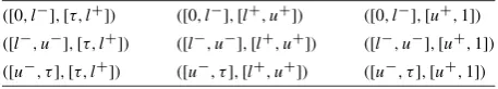
[image:7.544.49.458.273.503.2]

Thus, all combinations of intervals thatCτ(τ1−, τ2−)andCτ(τ1+, τ2+)could fall into are exhaustively enumerated in

(8)

[image:8.544.160.389.104.145.2]

Table 1

All combinations of intervals thatCτ(τ1−, τ2−)andCτ(τ1+, τ2+)could,

respectively, fall into

([0, l−],[τ, l+]) ([0, l−],[l+, u+]) ([0, l−],[u+,1]) ([l−, u−],[τ, l+]) ([l−, u−],[l+, u+]) ([l−, u−],[u+,1]) ([u−, τ],[τ, l+]) ([u−, τ],[l+, u+]) ([u−, τ],[u+,1])

3. Conceptions of various risk-based compromise operators

This section formally defines the various types of compromise operators we identified in the previous section. In particular, we discuss them in terms of how they reflect the users’ attitudes to risk in aggregation. We focus on risk here because it provides a well understood framework for characterising the types of nuance that are crucial to the flexible decision making we aim to capture [12,28,29]. In particular, we make the standard assumption that users can exhibit three broad types of attitude toward risk [53]: seeking (optimistic), averse (pessimistic) or risk-neutral (risk-neutral). In a specific application, users can choose a particular compromise aggregation operator according to the combination of these basic attitudes. That is, in the risk-seeking case the aggregated result is not smaller than the biggest rating, in the risk-averse case it is not bigger than the smallest rating, and in the risk-neutral case it is in-between the biggest and the smallest ratings. Formally, we have:

Definition 6.For a general compromise operatorCτ,

(1) it isτ-high-optimisticif∀τ₁+, . . . , τ_n+∈(τ,1],

Cτ(τ₁+, . . . , τn+)max{τ1+, . . . , τn+}; (24)

(2) it isτ-low-optimisticif∀τ₁−, . . . , τ_n−∈ [0, τ ),

τCτ(τ₁−, . . . , τn−)max{τ1−, . . . , τn−}; (25)

(3) it isτ-high-pessimisticif∀τ₁+, . . . , τ_n+∈(τ,1],

τCτ(τ₁+, . . . , τn+)min{τ1+, . . . , τn+}; (26)

(4) it isτ-low-pessimisticif∀τ₁−, . . . , τ_n−∈ [0, τ ),

Cτ(τ₁−, . . . , τn−)min{τ1−, . . . , τn−}; (27)

(5) it isτ-high-neutralif∀τ₁+, . . . , τ_n+∈(τ,1],

min{τ₁+, . . . , τ_n+}Cτ(τ₁+, . . . , τn+)max{τ1+, . . . , τn+}; (28)

(6) it isτ-low-neutralif∀τ₁−, . . . , τ_n−∈ [0, τ ),

min{τ₁−, . . . , τ_n−}Cτ(τ₁−, . . . , τn−)max{τ1−, . . . , τn−}. (29)

In the above definition, property (24) means that positive ratings are aggregated in a risk-seeking way; (25) that negative ratings are aggregated in a risk-seeking way; (26) that the positive ratings are aggregated in a risk-averse way; (27) that the negative ratings are aggregated in a risk-averse way; (28) that the positive ratings are aggregated in a risk-neutral way; and (29) that the negative ratings are aggregated in a risk-neutral way.

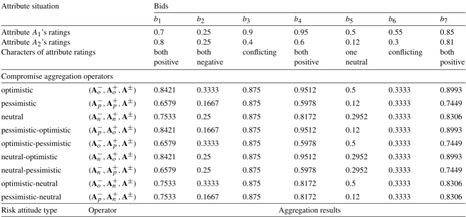
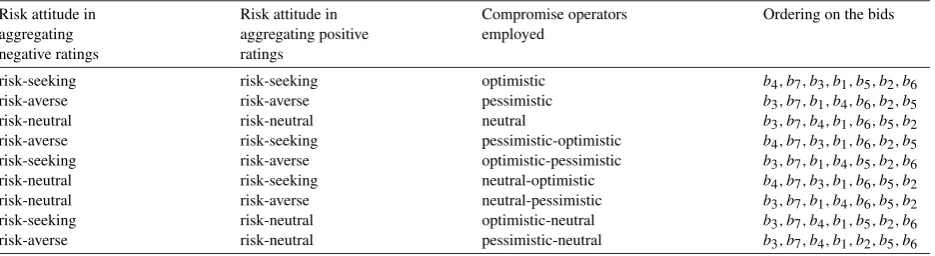
Since different decision makers may have different risk attitudes in aggregating positive or negative ratings, we have the following different concepts of compromise operator (which corresponds to the different cases in Table 1). Here we illustrate each of these attributes in terms of an auctioneer in a multi-attribute auction (see Section 7 for more details).

(9)

Suppose an auctioneer agent needs to aggregate a number of ratings (with respect to several attributes) to produce an overall rating for a bid. If it has a risking-seeking attitude in aggregating all its positive or all its negative ratings, an optimistic operator should be chosen. Thus, using such an operator to aggregate two positive ratings (for example 0.7 and 0.8) will produce an even more positive overall rating (for example 0.89), and using it to aggregate two negative ratings (for example 0.3 and 0.4) will produce a less negative overall rating (for example 0.47). Such an operator should be used if the decision maker does not fear over-rating an alternative when the individual ratings are all positive or all negative.

Definition 8.A general compromise operator ispessimistic, denoted asC(p)τ , if it isτ-low-pessimistic andτ -high-pessimistic.

If the auctioneer has a risking-averse attitude in aggregating all its positive or all its negative ratings, a pessimistic operator should be used. Using such an operator to aggregate two positive ratings (for example 0.7 and 0.8) will produce a less positive overall rating (for example 0.65), and using it to aggregate two negative ratings (for example 0.3 and 0.4) will produce an even more negative overall rating (for example 0.27). Such an operator should be used if the decision maker fears over-rating an alternative when the individual ratings are all positive or all negative.

Definition 9.A general compromise operator is optimistic-pessimistic, denoted asC(o-p)τ , if it isτ-low-optimistic andτ-high-pessimistic.

Sometimes an auctioneer’s risk attitude could differ depending on the decision being made. For example, when the two attributes’ ratings are both positive, it might be risk-averse since it fears over-rating the bid if, for example, it is not sure the bider can really deliver such an offer. However, when the two attributes’ ratings are both negative, it could be more risk-seeking since both rating are bad and so it would not rate it as being good even if it could give an overall rating higher than that of the individual ones. In other words, whatever the auctioneer did, it would not make a big mistake, but its optimistic rating might encourage the bider to continue bidding. In this case, an optimistic-pessimistic operator should be chosen. Thus, using such an operator to aggregate two positive ratings (for example 0.7 and 0.8) will produce a less positive overall rating (for example 0.65), and using it to aggregate two negative ratings (for example 0.3 and 0.4) will produce a less negative overall rating (for example 0.47).

Note that according to (21), (22) and Theorem 3, nullnorms are actually a kind of optimistic-pessimistic compro-mise operator. Moreover, in some special cases, the threshold element τ is also the annihilator (see Definition 5). Another interesting point is that from Lemma 1, we can see that these are exactly opposite to the case of uninorm compromise operators: in aggregating positive ratings decision makers are risk-seeking (optimistic), but in aggregat-ing negative rataggregat-ings they are risk-averse (pessimistic). So, in this sense, the uninorm compromise operator is a type of pessimistic-optimistic compromise operator:

Definition 10.A general compromise operator ispessimistic-optimistic, denoted asC(pτ -o), if it isτ-low-pessimistic andτ-high-optimistic.

If an auctioneer’s risk attitude varies from risk-averse in aggregating negative ratings, to risk-seeking in aggregating positive ratings, a pessimistic-optimistic operator should be chosen. Thus, using such an operator to aggregate two positive ratings (for example 0.7 and 0.8) will produce an even more positive overall rating (for example 0.85), and using it to aggregate two negative ratings (for example 0.3 and 0.4) will produce an even more negative overall rating (for example 0.27). Such an operator should be used if the decision maker’s attitude is influenced by the number of good or bad ratings received. Specifically, when all the attributes’ ratings are positive, it can model the phenomenon that the more of these there are, the more positive the agent becomes in its aggregating. Similarly, when all the ratings are negative, it can model the phenomenon that the more of these there are, the more negative the agent becomes.

(10)

neutral-optimistic, denoted asC(n-o)τ , if it isτ-low-neutral andτ-high-optimistic; it isneutral-pessimistic, denoted as C(n-p)τ , if it isτ-low-neutral andτ-high-pessimistic.

Here we only explain the first type of operator and others can be understood similarly. If an auctioneer’s risk attitude varies from risk-seeking in aggregating negative ratings, to risk-neutral in aggregating positive ratings, an optimistic-neutral operator should be chosen. Thus, using such an operator to aggregate two positive ratings (for example 0.7 and 0.8) will produce a tradeoff overall rating (for example 0.75), and using it to aggregate two negative ratings (for example 0.3 and 0.4) will produce a less negative overall rating (for example 0.47). Such an operator should be used if the decision maker wishes to encourage lower rated bids, while being more cautious with higher value ones. For example, if all the attributes’ ratings are negative, the auctioneer agent might offer encouraging feedback on the aggregation in order to try and elicit better subsequent bids. Whereas, when all the attributes’ ratings are positive, the auctioneer agent might want to give a more neutral feedback so that the bidder is encouraged to make a more favourable bid that increases its overall rating.

When taken together, these different compromise operators offer a rich set of possible ways (as shown in Table 1 in Section 7) in which individual ratings for a given alternative are combined to give an overall rating. This richness is important because different people have different attitudes toward risk [55] and if we want agents to fully act on their behalf then they must be capable of reflecting their individual nuances, preferences and attitudes to risk (see Section 7 for a more detailed example).

4. Properties of compromise operators

Having outlined the spectrum of possible compromise operators, we now consider their various properties. Firstly, we define the concepts ofτ-low andτ-high neutral elements as follows.

Definition 12.For a general compromise operatorCτ,

(1) e∈ [0,1]is said to be aτ-low neutral element if∀i∈ {1, . . . , n}, τ₁−, . . . , τ_i−₋₁,τ_i−₊₁, . . . , τ_n−∈ [0, τ],

Cτ(τ1−, . . . , τi−−1, e, τi−+1, . . . , τn−)=Cτ(τ1−, . . . , τi−−1, τi−+1, . . . , τn−); (30) (2) e∈ [0,1]is said to be aτ-high neutral element if∀i∈ {1, . . . , n},τ₁+, . . . , τ_i+₋₁, τ_i+₊₁, . . . , τ_n+∈ [τ,1],

Cτ(τ₁+, . . . , τ_i+₋₁, e, τ_i+₊₁, . . . , τn+)=Cτ(τ₁+, . . . , τ_i+₋₁, τ_i+₊₁, . . . , τn+). (31) Then in the following theorem we give the properties (with respect to the above two concepts) that lead a general compromise operator to become a specific type of compromise operator.

Theorem 4.For a general compromise operatorCτ,

(1) it isτ-high-optimistic ifτ is itsτ-high neutral element and∀τ₁+, . . . , τ_n+∈(τ,1],

Cτ(τ₁+, . . . , τn+)Cτ(τ₁+, . . . , τ_i+₋₁, τ, τ_i+₊₁, . . . , τn+); (32)

(2) it isτ-high-pessimistic if1is itsτ-high neutral element; (3) it isτ-low-optimistic if0is itsτ-low neutral element;and

(4) it isτ-low-pessimistic ifτ is itsτ-low neutral element and∀τ₁−, . . . , τ_n−∈ [0, τ ),

Cτ(τ1−, . . . , τn−)Cτ(τ1−, . . . , τi−−1, τ, τi−+1, . . . , τn−). (33)

Proof. In the following, we check them one by one:

Cτ(τ1+, . . . , τi+₋1, τ, τi+₊1, . . . , τn+)=Cτ(τ1+, . . . , τi+₋1, τi+₊1, . . . , τn+)

⇒Cτ(τ₁+, . . . , τn+)Cτ(τ, . . . , τ, τ_j+, τ, . . . , τ )=τ_j+

(11)

Cτ(τ₁+, . . . , τ_i+₋₁,1, τ_i+₊₁, . . . , τn+)=Cτ(τ₁+, . . . , τ_i+₋₁, τ_i+₊₁, . . . , τn+)

⇒Cτ(τ1+, . . . , τn+)Cτ(1, . . . ,1, τj+,1, . . . ,1)=τj+

⇒Cτ(τ₁+, . . . , τn+)min{τ1+, . . . , τn+};

Cτ(τ1−, . . . , τi−−1,0, τi−+1, . . . , τn−)=Cτ(τ1−, . . . , τi−−1, τi−+1, . . . , τn−)

⇒Cτ(τ₁−, . . . , τn−)Cτ(0, . . . ,0, τj−,0, . . . ,0)=τj−

⇒Cτ(τ₁−, . . . , τn−)max{τ1−, . . . , τn−};

Cτ(τ1−, . . . , τi−−1, τ, τi−+1, . . . , τn−)=Cτ(τ1−, . . . , τi−−1, τi−+1, . . . , τn−)

⇒Cτ(τ₁−, . . . , τn−)Cτ(τ, . . . , τ, τ_j−, τ, . . . , τ )=τ_j−

⇒Cτ(τ1−, . . . , τn−)min{τ1−, . . . , τn−}. 2

According to the above theorem, we can have the following two obvious corollaries.

Corollary 1.Ifτ ∈(0,1)is both theτ-low andτ-high neutral elements of a general compromise operatorCτ, then

the operator is a uninorm.

This corollary means that the concept of neutral elements (see Definition 1) is a special case ofτ-low andτ-high neutral elements.

Corollary 2. For a general compromise operatorCτ, if 0 is itsτ-low neutral element and1 is its τ-high neutral

element, then the operator is a nullnorm.

This corollary means that the concepts ofτ-low andτ-high neutral elements can not only cover the concept of neutral element, but also others. So, they are actually a kind of generalisation of neutral elements.

5. The construction of compromise operators

The previous two sections discussed the general concepts and properties of various compromise operators. Building on this, this section discusses the issue of how such operators can actually be constructed. More specifically, we give a number of ways to construct these operators from the existing t-norms, t-conorms and various compromise operators (and, actually, also reveal the relation of various compromise operators with these existing operators). We consider constructing these operators in this way because the standard principles of software and knowledge engineering have shown the benefits of reusing existing functions and operators to construct something new, rather than building from scratch.

The methods discussed in this section are of three broad kinds: the transfer-then-reverse method (Section 5.1), the additive generating function method (Section 5.2), and the ordinal sum method (Section 5.3). The idea behind the first method, which is widely used for constructing various aggregation operators, is to construct the new operators from existing operators basically by transferring functions and their reverse [9]. In the relevant literature, the second and third methods are, respectively, used: (i) to construct t-norms, t-conorms and uninorms from the ordinary sum operator (+) by means of so-called “additive generating functions” [21,22,38], and (ii) to construct new t-norms and t-conorms by setting the new operators as the ordinal sum of the existing operators [11,30,33]. In Sections 5.2 and 5.3, we discuss how the ideas behind these two methods can also be used to construct various compromise operators.

5.1. The transfer-then-reverse method

(12)

ratings. So, a specific compromise aggregation operator can be made of three components that are provided by these theorems, which will be illustrated at the end of this subsection.

First, we give the method that transfers existing t-norms and t-conorms to the compromise operator components of aggregating all negative or all positive ratings.

The properties of the transfer functions are listed in the following definition:

Definition 13.For a givenτ ∈ [0,1],

(1) a non-decreasing 1–1 mappingh:[0, τ] → [0,1]is aτ−-constructor ifh(0)=0 andh(τ )=1; and (2) a non-decreasing 1–1 mappingh:[τ,1] → [0,1]is aτ+-constructor ifh(τ )=0 andh(1)=1.

The method of transferring t-norms and t-conorms is given in the following theorem:

(1) it isτ-high-optimistic if∀τ₁+, . . . , τ_n+∈(τ,1],

Cτ(τ1+, . . . , τn+)=h−1

S(h(τ₁+), . . . , h(τ_n+)), (34)

wherehis aτ+-constructor;

(2) it isτ-low-optimistic if∀τ₁−, . . . , τ_n−∈ [0, τ ),

Cτ(τ₁−, . . . , τn−)=h−1

S(h(τ₁−), . . . , h(τ_n−)), (35)

wherehis aτ−-constructor;

(3) it isτ-high-pessimistic if∀τ₁+, . . . , τ_n+∈(τ,1],

Cτ(τ₁+, . . . , τn+)=h−1

Th(τ₁+), . . . , h(τ_n+), (36)

wherehis aτ+-constructor;and

(4) it isτ-low-pessimistic if∀τ₁−, . . . , τ_n−∈ [0, τ ),

Cτ(τ₁−, . . . , τn−)=h−1

Th(τ₁−), . . . , h(τ_n−), (37)

wherehis aτ−-constructor.

Proof. Here we only show the case of theτ-high-optimistic operator since the others can be derived in a similar manner.

Sh(τ₁+), . . . , h(τ_n+)maxh(τ₁+), . . . , h(τ_n+)

⇒h−1Sh(τ₁+), . . . , h(τ_n+)h−1maxh(τ₁+), . . . , h(τ_n+)

=maxh−1h(τ₁+), . . . , h−1h(τ_n+)

=max{τ₁+, . . . , τ_n+}. So, by Definition 6, item 1 of the theorem holds. 2

To illustrate the above method, we give the following example:

Example 4.Some examples of t-norms and t-conorms are listed as below.

(1) Idempotent operators:

TI(a1, . . . , an)=min{a1, . . . , an}, (38)

(13)

(2) Probability operators:

TP(a1, . . . , an)= n

i=1

ai, (40)

SP(a1, . . . , an)=1− n

i₌1

(1−ai). (41)

(3) Dombi operators:

TD(a1, . . . , an)=

1 n

i=1a1i −(n−1)

, (42)

SD(a1, . . . , an)=1−

1 n

i=11−1ai −(n−1)

. (43)

(4) Lukasiewicz operators:

TL(a1, . . . , an)=max

0, n

i=1

ai−(n−1)

, (44)

SL(a1, . . . , an)=min

1, n

i=1

ai

. (45)

Clearly, the following is aτ+-constructor:

h(x)= 1

1−τ(x−τ ). (46)

Thus, by Theorem 5, from t-conorm operators (39), (41), (43) and (45), we can use (46) to obtain the following τ-high-optimistic operators:

C(o)_{(I )τ}(τ₁+, . . . , τ_n+)=(1−τ )maxn i=1

1 1−τ(τ

+

i −τ )+τ, (47)

C(o)_{(P )τ}(τ₁+, . . . , τ_n+)=(1−τ )

1−

n

i=1

1− 1

1−τ(τ

+

i −τ )

+τ, (48)

C(o)_(D)τ(τ₁+, . . . , τ_n+)=(1−τ )

1− 1

n i=1

1−τi+−τ 1−τ

₋1

−(n−1)

+τ, (49)

C(o)_(L)τ(τ₁+, . . . , τ_n+)=(1−τ )min

1, n

i=1

1 1−τ(τ

+

i −τ )

+τ, (50)

whereτ₁+, . . . , τ_n+∈(τ,1].

Actually, by Theorem 5 we can also construct various compromise operators from the existing uninorm operator. This is because by the following theorem that can easily be proved, we can construct some t-norm and t-conorm operators from uninorm operators first.

Theorem 6.The following[0,1] × [0,1] → [0,1]mappings defined through uninorm operatorUτ are, respectively,

t-norm and t-conorm operators:

TU(x, y)=h−₁1

Uτ

h1(x), h1(y)

, (51)

SU(x, y)=h−₂1

Uτ

h2(x), h2(y)

, (52)

(14)

Second, we give the method that transfers existing averaging operators to the compromise operator components of aggregating all negative or all positive ratings.

The properties of the transfer functions are given in the following definition:

(1) a non-decreasing 1–1 mappingh:[0, τ] → [0, τ]is aτ−-generator ifh(0)=0 andh(τ )=τ; and (2) a non-decreasing 1–1 mappingh:[τ,1] → [τ,1]is aτ+-generator ifh(τ )=τ andh(1)=1.

(1) it isτ-high-neutral if∀τ₁+, . . . , τ_n+∈(τ,1],

Cτ(τ1+, . . . , τn+)=h−1

Mh(τ₁+), . . . , h(τ_n+), (53)

wherehis aτ+-generator; and

(2) it isτ-low-neutral if∀τ₁−, . . . , τ_n−∈ [0, τ ),

Cτ(τ₁+, . . . , τn+)=h−1

Mh(τ₁−), . . . , h(τ_n−), (54)

wherehis aτ−-generator.

Proof. Here we only show the case of theτ-high-neutral operator since the others can be derived in a similar manner.

minh(τ₁+), . . . , h(τ_n+) Mh(τ₁+), . . . , h(τ_n+)maxh(τ₁+), . . . , h(τ_n+)

⇒h−1minh(τ₁+), . . . , h(τ_n+) h−1Mh(τ₁+), . . . , h(τ_n+)h−1maxh(τ₁+), . . . , h(τ_n+)

⇒min{τ₁+, . . . , τ_n+} =minh−1h(τ₁+), . . . , h−1h(τ_n+) h−1Mh(τ₁+), . . . , h(τ_n+) maxh−1h(τ₁+), . . . , h−1h(τ_n+)

=max{τ₁+, . . . , τ_n+}. So, by Definition 6, item 1 of the theorem holds. 2

Third, we give the method that transfers uninorm and averaging operators to the compromise operator components of aggregating conflicting ratings.

The properties of transfer functions are listed in the following definition:

(1) a non-decreasing 1–1 mappingh:[0,1] → [0,1]is aτ-generator ifh(0)=0,h(τ )=τ andh(1)=1; and (2) a non-decreasing 1–1 mappingh:[0,1] → [0,1]is a[0,1]-generator ifh(0)=0 andh(1)=1.

The method is given in the following theorem:

(1) it is uninorm-like if∀τ₁−, . . . , τ_m−∈ [0, τ],τ₁+, . . . , τ_n+∈(τ,1],

Cτ(τ1−, . . . , τm−, τ1+, . . . , τn+)=h−

1

Uτ

h(τ₁−), . . . , h(τ_m−), h(τ₁+), . . . , h(τ_n+), (55)

wherehis aτ-generator;and

(2) it is averaging-like if∀τ₁−, . . . , τ_m+∈ [0, τ],τ₁+, . . . , τ_n+∈(τ,1],

Cτ(τ₁−, . . . , τm−, τ1+, . . . , τn+)=h−1

Mh(τ₁−), . . . , h(τ_m−), h(τ₁+), . . . , h(τ_n+), (56)

(15)

Proof. Here we only show the case of uninorm-like operator since the others can be derived in a similar manner.

τ₁−τ, . . . , τ_m−τ, τ₁+τ, . . . , τ_n+τ

⇒h(τ₁−)h(τ )=τ, . . . , h(τ_m−)h(τ )=τ, h(τ₁+)h(τ )=τ, . . . , h(τ_n+)h(τ )=τ

⇒minh(τ₁−), . . . , h(τ_m−), h(τ₁+), . . . , h(τ_n+) Uτ

h(τ₁−), . . . , h(τ_m−), h(τ₁+), . . . , h(τ_n+) maxh(τ₁−), . . . , h(τ_m−), h(τ₁+), . . . , h(τ_n+)

⇒minτ₁−, . . . , τ_m− =h−1minh(τ₁−), . . . , h(τ_m−) h−1minh(τ₁−), . . . , h(τ_m−), h(τ₁+), . . . , h(τ_n+) h−1Uτ

h(τ₁−), . . . , h(τ_m−), h(τ₁+), . . . , h(τ_n+) h−1maxh(τ₁−), . . . , h(τ_m−), h(τ₁+), . . . , h(τ_n+) h−1maxh(τ₁+), . . . , h(τ_n+) =max{τ₁+, . . . , τ_n+};

h−1Uτ

h(τ₁−), . . . , h(τ_m−), h(τ ), h(τ₁+), . . . , h(τ_n+)

=h−1Uτ

h(τ₁−), . . . , h(τ_m−), τ, h(τ₁+), . . . , h(τ_n+)

=h−1Uτ

h(τ₁−), . . . , h(τ_m−), h(τ₁+), . . . , h(τ_n+). So, by Definition 4, item 1 of the theorem holds. 2

Finally, we illustrate how to use the above methods to construct several specific kinds of compromise operators (the rest of them can be discussed similarly). In particular, the following example shows how to use the above methods to construct optimistic compromise operators from t-conorm, uninorm and averaging operators.

Example 5.Forτ∈(0,1), clearly

h1(x)=

1

τx, (57)

h2(x)=

1

1−τ(x−τ ), (58)

h3(x)=x, (59)

h4(x)=sin

π 2x

(60)

are, respectively, aτ−-constructor, aτ+-constructor, aτ-generator, and a[0,1]-generator. Then by Theorems 5 and 8, and Definition 7, from Dombi t-conorm (43), uninorm (7), arithmetical mean (11), (46), and (57)–(60), we have the following uninorm-like and averaging-like optimistic compromise operators:

C(o)τ (a1, . . . , an)= ⎧ ⎪ ⎪ ⎪ ⎪ ⎪ ⎪ ⎨ ⎪ ⎪ ⎪ ⎪ ⎪ ⎪ ⎩

τ1−n 1

i=1₁₋11

τ ai−

(n−1)

ifa1, . . . , an∈ [0, τ],

(1−τ )1−n 1

i=1₁₋ 11 1−τ(ai−τ )

−(n−1)

+τ ifa1, . . . , an∈(τ,1],

1 1+(₁₋τ_τ)n−1n

i=1 1−ai

ai

otherwise;

(61)

C(o)_τ (a1, . . . , an)= ⎧ ⎪ ⎪ ⎪ ⎪ ⎨ ⎪ ⎪ ⎪ ⎪ ⎩

τ1−n 1

i=1₁₋11

τ ai−

(n−1)

ifa1, . . . , an∈ [0, τ],

(1−τ )1−n 1

i=1₁₋ 11 1−τ(ai−τ )

−(n−1)

+τ ifa1, . . . , an∈(τ,1],

2

πarcsin ₁

n n

i=1sin

_π

2ai

otherwise.

(16)

The following example shows how to use the proposed method to construct an optimistic-neutral compromise operator.

Example 6.By Theorems 5 and 8, from Dombi t-conorm (43), uninorm (7), arithmetical mean (11), (57), (59) and τ+-generatorh(x)= 1

1+1_τ(1−x) we have the following uninorm-like optimistic-neutral compromise operator:

C(oτ-n)(a1, . . . , an)= ⎧ ⎪ ⎪ ⎪ ⎪ ⎪ ⎨ ⎪ ⎪ ⎪ ⎪ ⎪ ⎩

τ1−n 1

i=1₁₋11

τ ai−

(n−1)

ifa1, . . . , an∈ [0, τ],

τ +1− 1 τ

n n

j=1₁₊11

τ (1−aj )

ifa1, . . . , an∈(τ,1],

1 1+₁₋τ_τn−1n_i₌₁1−ai

ai

otherwise.

(63)

5.2. The additive generating function method

In the relevant literature, the method is mainly used to construct t-norms, t-conorms and uninorms from the ordinary sum operator (+) by means of so-called “additive generating functions” [21,22,38]. Actually, the idea behind the method can also be used to construct various operators. In fact, by Theorems 5, 6 and 8, we can also construct various types of compromise operators in this way (i.e., using “additive generating functions” to construct t-norms, t-conorms and uninorms first and then using them further to construct various compromise operators). Moreover, we can directly construct various compromise operators in this way as follows:

Theorem 9.Letg1be a mapping from[0, τ]to(−∞,0],g2be a mapping from[τ,1]to[0,+∞), andg3a mapping from[0,1]to(−∞,+∞). Then for a particular mappingC+_τ :_n_∈N[0,1]n_{→ [}₀_,₁_]_{that is defined as}_:

C+τ(a1, . . . , an)= ⎧ ⎪ ⎨ ⎪ ⎩

g−₁1(g1(a1)+ · · · +g1(an)) ifa1, . . . , an∈ [0, τ], g−₂1(g2(a1)+ · · · +g2(an)) ifa1, . . . , an∈(τ,1], g−₃1(g3(a1)+ · · · +g3(an)) otherwise,

(64)

ifg3is strictly increasing, bijective, and hasg3(τ )=0, it is a compromise operator; and further:

(1) it isτ-high-optimistic ifg2is strictly increasing, continuous andg2(τ )=0andg2(1)= +∞;

(2) it isτ-low-optimistic ifg1is strictly decreasing, continuous andg1(0)=0;

(3) it isτ-high-pessimistic ifg2is strictly decreasing, continuous andg2(1)=0;and

(4) it isτ-low-pessimistic ifg1is strictly increasing, continuous andg1(τ )=0andg1(0)= −∞.

Proof. We only show the operator is a general compromise operator according to Definition 4 since the others can easily be shown.

(1) Conflict:

0τ₁−< τ, . . . ,0τ_k−< τ, τ < τ₁+1, . . . , τ < τ_l+1

⇒g3(0)g3(τ₁−) < g3(τ )=0, . . . , g3(0)g3(τ_k−) < g3(τ )=0,

0=g3(τ ) < g3(τ₁+)g3(1), . . . ,0=g3(τ ) < g3(τ_l+)g3(1)

⇒ming3(τ₁−), . . . , g3(τ_k−)

g3(τ₁−)+ · · · +g3(τ_k−)+g3(τ₁+)+ · · · +g3(τ_l+)max

g3(τ₁+), . . . , g3(τ_l+)

⇒min{τ₁−, . . . , τ_k−} =g₃−1ming3(τ1−), . . . , g3(τk−) g₃−1g3(τ₁−)+ · · · +g3(τ_k−)+g3(τ₁+)+ · · · +g3(τ_l+)

g₃−1maxg3(τ₁+), . . . , g3(τ_l+) =max{τ₁+, . . . , τ_l+}

(17)

(2) Boundary condition:

C+_τ(0, . . . ,0)=g₁−1g1(0)+ · · · +g1(0)

=g₁−1g1(0)

=0,

C+τ(1, . . . ,1)=g2−1

g2(1)+ · · · +g2(1)

=g₂−1g2(1)

=1.

(3) Monotonicity: because of the monotonicity of g1 and g2, it is clear that ∀a1, a₁, . . . , an, an ∈ [0,1], a1

a₁, . . . , anan ⇒C+τ(a1, . . . , an)C+τ(a1, . . . , an); (4) Symmetry:∀a1, . . . , an∈ [0,1], clearly

{p1, . . . , pn} = {1, . . . , n} ⇒C+τ(a1, . . . , an)=C+τ(ap1, . . . , apn). 2 5.3. The ordinal sum method

In the relevant literature, this method is mainly used to construct t-norms and t-conorms by setting the new oper-ators as the ordinal sum of the existing ones [11,30,33]. Actually, the idea behind this method can also be used for constructing various types of compromise operators from existing ones. In fact, by Theorem 5, we can obtain t-norms and t-conorms from existing compromise operators, then the ordinal sum of these compromise operator based t-norms and t-conorms can constitute new t-norms and t-conorms, and finally by Theorem 5, we can obtain new compromise operators from the ordinal sum t-norms and t-conorms.5

6. The construction of uninorm compromise operators

From the above section, we can see that uninorm compromise operators play an important role in constructing var-ious compromise operators. This means if we have more uninorm operators we can have more compromise operators. Given this, this section explores the issue of constructing uninorms and gives a specific method for so doing.

Firstly, we need the following lemma that is a basic fact in modern algebra [49].

Lemma 5.Let(◦, X)and(, Y )be two algebraic structures. If

y1y2=f−1

f (y1)◦f (y2)

,

where mappingf:X→Y is a1–1and increasing, and operator◦is increasing, associative and commutative, then operatoris increasing, associative and commutative.

Before delving into the method, we need a sort of generating function concept:

Definition 16.For a givenτ ∈(0,1), a 1–1 non-decreasing functionhτ:[−1,1] → [0,1] is a[−1,1]-generator if hτ(−1)=0,hτ(0)=τ andhτ(1)=1.

Now we can detail our method:

Theorem 10.The following is a uninorm compromise operator with a neutral element of0.5:

U0.5(a1, a2)=

h−1(U(P )τ (h(2a1−1), h(2a2−1)))+1

2 , (65)

wherehis a[−1,1]-generator.

Proof. Letg(x)=2x−1, and thusg−1(x)=x+₂1. And letf (x)=h(g(x)), and thusf−1(x)=g−1(h−1(x)). Then we can rewrite (65) as

U0.5(a1, a2)=f−1

U(P )τ

f (a1), f (a2)

. (66)

So, by Lemma 5 and (1) that definesU(P )τ , commutativity, associativity and monotonicity hold forU0.5. In order to

prove thatU0.5is a uninorm, by Definition 1, we need to further check that: