THE USE OF OPTICAL ABERRATION COEFFICIENTS
by
P. W. FORD B. Sc (Hons.)
A Thesis submitted for examination for the degree . of
DOCTOR OF PHILOSOPHY
UNIVERSITY OF TASMANIA
Contents
Introduction
Part I SUMMARY OF 'THEORY
1• Sign Conventions. Aberrations of a Ray 1
Paraxial Coefficients
4
Aberration Coefficients
8
"a" and "b" Aberration Coeffidients 13 Calculation of Aberration Coefficients 21
Intrinsic Coefficients 30
Part' II
COMPUTER AND PROGRAMMES
Computer Description
34
Aberration Coefficients Programme
40
Ray Trace Programme
45
Predicted Displacements from Aberration Coefficients
59
Part III NUMERICAL RESULTS
Specifications of Systems Examined 63 Calculations Performed on the Optical Systems
69
Quality of Agreement between q and 0[2], 0[3] 72 Criteria Indicating Accuracy of Predicted-
Contents
Part IV
APPLICATION OF ABERRATION COEFFICIENTS
Use of Coefficients 86
Derivatives of the Coefficients
93
APPENDIX 1
Final Aberration Coefficients of Tessar 96
APPENDIX 2
Portion of Biotar 12° Ray Trace Results
97
APPENDIX
3
Portion of Biotar 12° Predicted Displacements 98
APPENDIX
4
Formulae Used in Aberration Coefficients Programme 99
INTRODUCTION.
An extensive theory of aberration coefficients of
symmetrical optical systems has been developed by Buchdahl in his
monograph "Optical Aberration Coefficients - (hereafter called M) and
3,•99.
extended in subsequent papers, 2, The advantages resulting from
the use of these coefficients rest in two important properties.
Firstly, the one set of coefficients characterise systems of rays,
that is, they apply simultaneously to all rays that traverse the
optical system. Secondly the aberration coefficients are the suns
of corresponding coefficients computed for each surface of the system
(the contributions to the coefficients). This enables the action of
the system on all rays to be analysed surface
hy
surface and it isthis that places a powerful tool in the hands of the designer.
Now, although there is only one set of coefficients for
each system, it is an infinite set. Obviously the calculation of
them all is impossible. So far, computing schemes have been designed
for the computation of all the third, fifth and seventh order
monochromatic coeff1cients4, the coefficients of ninth
5 and eleventh9
order spherical aberration, and several of the more important
chromatic coefficients (M Chapter XIII). Naturally, the aberrations
of a system are not completely described by only these coefficients.
The object of this thesis is to examine the effectiveness
of the first three orders of the monochromatic coefficients in the
description of the aberrations of optical systems. As well as
enabling a detailed analysis of a system, the coefficients and their
surface contributions are of considerable use in the differential
correction of a system following the initial design. The effectiveness
of the coefficients in this field is also examined here.
The work has been restricted to monochromatic coefficients,
II
out in monochromatic light. Also, the systems studied here have been
restricted to those containing spherical surfaces only. The extension
of the work to aspherical surfaces is a matter of detail and not of
method; as mentioned in M Section
55,
the only change is that the"intrinsic" coefficients (Section
5, 6
of this thesis) containadditional terms which depend on the "extra-axial" curvatures of the
aspheric surfaces. These additional terms in no way affect the
general theory or the application of the coefficients. The aberration
coefficients in no way indicate whether the system they represent is
aspheric or not. However, in the construction of computing schemes
for the coefficients, many simplifications can be introduced if only
spherical surfaces are being considered, resulting in comparatively
short schemes, e.g. compare M 81.3 with 84.23, 33, 44.
Since the publication of M, several misconceptions have
occurred regarding the coefficients and the contributions to them by
the surfaces, Some of these have been discussed in a paper by
Cruickshank and Hills10. It is probable that these erroneous
Impressions have occurred as a result of 1) the multiplicity of
symbols used in M, and 2) the iterative method used to derive the
expressions for the coefficients.
About the symbolism little can be done. As mentioned in
the preface to M "higher-order optics is a battle of symbolism, not
of advanced mathematics." Consequently, where type allows, the
symbolism in this thesis is that of M. The most notable exception
is the use here of single and double underlines, the symbols so
marked representing the bold-face type and the Gothic script of M
respectively.
Iteration is quite familiar; everyone is acquainted with
Newtons method for obtaining square roots, in which successively
III
iterative step. Perhaps as a result of this application, some workers have supposed that the aberration coefficients are
approximate. This is entirely incorrect. As in the square root _ procedure, approximation is involved only by virtue of the fact that an infinite series has been terminated without regard to the remaining terms. The aberration coefficients are the coefficients of the terms In the infinite power series expansion for the "displacement" of a ray (See Section 1). When this series is terminated, we have only
an approximation of the displacement. It is the accuracy of this •
approximation that is being examined here. However, the coefficients of the series are exact. After each iterative step explicit
expressions for new higher-order coefficients are obtained, not better
approximations of earlier ones.
Failure to realise this may have arisen as a result of the iteration in M being applied to a series containing more than one variable, which necessarily involves a large number .of symbols. Therefore in Part I of this thesis two examples of iteration are presented, the second being more complex than the first. The second example introduces the idea of "intrinsic" coefficients, these being the basic coefficients from which all others are obtained. It is hoped that these examples will lead to a clearer understanding of the methods used in M.
By choosing suitable coordinates with which to specify a ray, considerable advantages ensue both in the computation and application of the aberration coefficients. These coordinate
systems and the advantages thereof are also presented in Part I along with the basic theory of the coefficients.
The examination of the effectiveness of the coefficients in describing the aberrations of a number of representative systems
IV
calculations were performed on desk machines and it was obvious from
the outset that this was too slow. For instance, a set of third,
fifth and seventh order coefficients for a six surface system
occupied two girls for four days. Thus my first task here was to
learn to programme an electronic computer to perform this and other
calculations. Accordingly, an approach was made to the University
of New South Wales for the use of their machine, an English Electric
"DEUCE". As a result of their very generous assistance, in about
nine months I had written a programme for the computation of the first
three orders of coefficients, which, incidentally, almost exceeded
the 8,000 word capacity of the machine. It has subsequently been
rewritten to achieve a reduction in computing time of about 20 percent.
Using this programme, the coefficients for a six surface system can
be obtained in about 5 minutes machine time.
Following this, two more programmes were written, one for
general ray tracing and the other for the computation of the
displacement of a ray using the aberration coefficients. Apart
from a few special trignometric ray traces, the entire numerical work
in this thesis is based on the results of these three programmes.
Since these programmes were designed for general use in
optical design, they have all been coded in basic machine language.
The increase in time and expense for the programming is more than
offset by the considerable economies in machine time realised during
their subsequent extensive use.
The "DEUCE" is an interesting machine in that it uses
mercury acoustic delay-lines for the high speed stores 'with a
magnetic drum as the backing store. Notwithstanding this rather
slow type of high speed storage the machine is quite fast in its
operation. This is due mainly to the high digit frequency
(1 megacycle), the arrangement of the arithmetic units and the
considerable amount of information contained in one instruction word.
The first section of Part II describes the design and operation of
V
the three programmes written for it.
In Part III the accuracy of the first three orders of aberration coefficients in describing the aberrations of optical systems is examined. Six modern photographic objectives have been used for this work. This is an extension of the work presented in
a paper6 by Buchdahl in which he uses two systems as illustration, one of wide field and the other of large aperture. The quality of the predicted displacements has been judged on the appearance of tangential curves, annular curvesand spot diagrams plotted for several pencils in each of the six systems.
In the tangential and annular curves are plotted the
displacements of rays predicted from the first two and the first three orders of coefficients, as well as the true displacements obtained from ray traces, Predicted displacements calculated using the first three orders only are used in the spot diagram comparisons. The results of the comparisons have been tabulated in Part III (Table V).
It would be of advantage to the optical worker if some simple criterion could be found which would indicate the reliability of the coefficients in predicting displacements of rays. One such criterion, which I have termed an "angle criterion" was suggested in reference 6, "It is a matter of experience that reliance cannot be placed on the values of the predicted displacements if some Isin II
or isin VI (in a ray trace) exceed a value of about 0.8". This and other angle criteria have been examined in the light of the six
VI
Part IV deals with the methods of application of the
aberration coefficients in the analysis and differential correction of optical systems. These are the important applications; the mere construction of curves and spot diagrams can be done by ray
tracing, which, however does not give any indication of why the
system performs as it does, or how to improve it. On the other hand, the aberration coefficients and their derivatives, which characterise systems of rays, can indicate which surfaces require modification and as well can indicate with considerable accuracy the effect of
simultaneous changes of parameters at several surfaces. When it is known that the coefficients adequately describe the aberrations of a
system, their use is quite straight forward and is described in the paper by Cruickshank and Hills100 This is summarised in Part IV.
However, the main work in this part is concerned with a method that can be used when the first three orders of coefficients
do not in themselves adequately describe the system. The method is based on a property of the coefficients which arises from the
processes used in initial design. As a result of this property, it is still possible to analyse a system and to predict the effect of
changes of parameters even when the coefficients are known not to adequately represent the aberrations. The method is illustrated using two of the systems already described in Part III.
1n order to use the coefficients to predict the effect of changes of parameters, it is necessary to know at least the first
VII
If second derivatives are required then the theory presented in M will
have to be developed. However, a knowledge of the first derivatives
of the third, fifth and seventh order coefficients enables the effect
of 5 percent changes to be predicted satisfactorily. These
derivatives can be obtained by numerical means using the aberration
coefficients programme. The accuracy of this method is discussed
and illustrated with use of a cemented doublet. With the aid of
certain identities between the derivatives and coefficients, deveiloped
from the theory in M, it is shown that the first derivatives can be
VIII
Acknowledgements.
I wish to thank my supervisor, Dr. F. D. Cruickshank, for
his interest in the progress of this work. As an experienced optical
designer, his discussions on the problems confronting optical workers
were very helpful in indicating the type of work to be undertaken in
this thesis. It was also under his auspices that the many trips to
use the computer in Sydney were made possible.
The numerous discussions with Dr. H. A. Buchdahl concerning
the theoretical and practical aspects of the aberration coefficients
were invaluable. I cannot speak too highly of his assistance in this
work, without which my task would have been much more difficult.
I am very grateful to the staff in charge of the "DEUCE"
computer at the University of New South Wales, Sydney, for the way in
which they placed their facilities at my disposal. Several times
they worked overtime and rearranged time schedules to accommodate me,
often at rather short notice. It was a pleasure to work with them.
I am indebted to Mrs. B, Brown who carried out the
auxiliary calculations used in this work. She also assisted in
checking the coding and card—punching of the various programmes, as
well as computing the results necessary to check their initial
operation.
My thanks go to two typists, Mrs. P. Top and Mrs. G. Harman
who cheerfully undertook the often complex typing of the manuscript.
Finally, I would like to acknowledge the generous assistance
of the staff of the Photographic Department who carried out the
1,
PART I - Surmnarz of Theory
1. Sign Conventions. Aberrations of a Ray.
In M and this thesis, the following conventions for
symbols and subscripts are used. Upper case letters refer to
quantities associated with finite rays before refraction at a surface,
the surfaces themselves being specified by subscripts 1, 2, • , •
.0, k. The subscript k always refers to the last surface,
Primed ( 1 ) upper case letters denote the corresponding quantities
after refraction. Lower case letters refer to quantities
associated with rays lying everywhere in the infinitesimal
neighbourhood of the axis (paraxial rays), that is, to quantities
determined only by the laws of paraxial optics. All superscript
and subscript conventions apply similarly to paraxial and
non-paraxial syMbols. Unless otherwise stated, symbols from which the
surface subscript is omitted refer to quantities at au surface.
These are the principal conventions which apply throughout, but
additional superscripts and subscripts will be introduced as required.
Associated with each surface of the system is a
left-handed set of rectangular cartesian axes with the origin at
the pole of the surface. The x-axes of these coordinate systems
lie along the axis of symmetry of the optical system, the positive
direction being that in which light proceeds through the system.
All the y-axes lie in the meridional plane. Let Om be the
axial point of a plane, A, in the object space, normal to the axis,
Then rays from Om [iim ,0,0] whose paths through the system are
determined only by the laws of paraxial optics, will intersect
the axis in the final image space at a point
ol& (7.01( . o
t
o].
0(1k is
defined as the axial point of the ideal image plane bl/ ,conjugate to Ft. Select any point 01 in the object plane Fi
and denote its coordinates by (Im (Fig.1). By
definition, if the optical system were perfect, all rays from 0,
2,
Pi in some point J whose coordinates [74 ,-hjk ,-hik ] would be
such that
where mg is a constant of the system independent of Hy, , Hzi *
called the paraxial magnification for the conjugate planes PI,
J is called the
umi_image.mint
conjugate to 0,and hik, hik the ideal image heights. In actual practice,
however, a ray from 0, will not, in general, pass through J,
but through some neighbouring point Og {7.sJk , °RA ). The
aberration qk sik (F1g02) of the ray is defined as
e j1k =Hjk— hjk , elk = hzic
To simplify the writing, all symbols singly underlined shall be
taken as referring to both the y- and z- components of the quantity
in question. Hence the preceding equation will be written
Since each refracting surface has an object and image plane
conjugate to PI, the jth image plane being also the 0 +0th
Object plane, the aberrations of a ray can be defined at these
planes in a manner similar to (1.1). Thus, at the jth object
plane,
ej (1.2)
and at the jth image plane
to
cg
c
..,
a
c
a.
to
Fr
....
u
.=
Cr
I
0
00
Coordina te sys tem and c anon ic a l c oordina te s
a
0.
"6
›-
ray intersection point
Pig. 2 Aberrations (or displacements)
3
0A ray incident at any surface will be specified by the four
canonical variables "T, Z, V. W. Y and Z are cartesian
coordinates of the point of intersection of the ray with the plane
tangent to the refracting surface at its pole while V and W are
related to the direction cosines (cxj3,y) of the ray by the
expressions
V = -PAk. W (1?
whence it follows that
i
= ii 4. w2 -2 . 105)
In accordance with the convention just introduced Y is to be
Interpreted as standing for both Y and Z, and V as standing
for both V and W.
If i s i,i are the coordinates of a current point on a
ray, then the equation of the ray may be written
Yr = Y V i (1 9 6)
If we put = di, the axial distance between surfaces j and
j f s, then Yr will bethe coordinates of the point of intersection
of the ray with the (j+1 )th polar tangent plane,
Thus
Yj 4.1 d/V1 ;
•
It is convenient to omit the subscript j and to replace the
subscript j + 1 simply by the subscript +. Then we have
4.
Equations (1.7) are 'the transfer equations for canonical variables.
2. Paraxial Coefficients
Defining the symbol A to be the change in a quantity
on refraction at a surface e.g. AX = X' - X, it is shown in M
Section
4
thatI cY - V (2.1)
A (N a I) = 0 (2.2)
and also AY = xAV (2.3)
where c (=1/r) is the curvature of the surface. For paraxial
rays these relations reduce to
ANi = 0
eAy = (1 v) (2.4)
since a,a1-,- 1, xAV
Using (2.4) and (1.7) we get the paraxial recurrence
relations
(1-k)cd 9 1y kd'v
= (1 - k)c y kv ( 2. 5 )
where k = N/N 9 .
Thus we can obtain 39+1 vi+1 from 39 , vi. Since
Yj+s, vh,. are linearly related to yj, vj, then yj, vj are
linearly related to yi, vi and the constants involved depend
only on the constitution of the system. Hence
Yi = Ypi Yi. + Ycri
vj = Vpj yi + Vqj Vt
the yo 9 Yqi, Vpi 9 Vqj being called the "paraxial coefficients" of the jth surface. Notice that the relations for yj and zj contain the same coefficients, and that the same is true of the expressions for vj and wj. Other paraxial coefficientscan be formed from these by linear combination, e,g,
ipj c yps voi
(2. 7 )
C iqj ■•• Vqj
so that
ij = ipj iqj vi (2.8)
and these will be used as the need arises.
The paraxial "p" coefficients can be most easily obtained by tracing a ray by means of (2.5) whose formal starting data are
yi = 1, vi = 0 (p-ray). Then the values of y, v at each surface are yp, vp. Similarly the "q" coefficients can be Obtained by tracing a second ray naving the starting data yi = 0,
=1 (q-ray).
An important identity between the paraxial coefficients is obtained as follows.
Consider two ApbAIrary: paraxial rays, one of which is a tangential ray, denoted by a bar over the symbols. Defining a quantity W by
X = N(kr iry), (2. 9)
then it is shown in M Section 5(b) that X is an optical
invariant, that is, its value is constant ‘ throughout the systeM for the pair of rays considered. If, in (2.9), the tangential ray is one from the axial point of the object, and the second ray passes through the Object point, then X. can be shown to be the
Lagrange invariant, i.e. X = Nveh. Expressing the paraxial
variables in (2.9) in terms of their values at the first surface
by means of (2.6), one obtains
Xi i‘Tj N1 ) (Ypj Vqj Yqj Vpi )?ti
Since X i = Xi
ypi vqj yqi Vpj = icr/NJ (2 0 10)
Apart from enabling the computation of the paraxial
coefficients to be checked, this identity (2,10) is very useful
In the simplification of many expressions which occur in the
development of the aberration coefficient theory. Several.other
Identities can be obtained from it, for example
vp vci — vo vli = c Ni (k - 41)/N (201)
yp vet -:, yq vpg = N1 /N I (2.12)
yp iq - yq ip = -NI /N . (2.13)
To simplify the notation, we introduce the convention
that if a prime is attached to the left of a symbol, then the
symbol is divided by M. Such a prime will be termed an
ante-prime. Thus (2.10) becomes
yp vq. yq Vp = 1/ 1 1Sr . 2.14)
The identity (2.14) is used in the following derivation for the
focal lengths of an optical system.
Let the axial points of the front and rear principal
planes be Po and Pj respectively, these planes, P,P I , having
arctan
Po p
f t
Fig. 3
Posterior focal length
Fig. L.
[image:21.679.72.622.63.833.2]and
(2.16)
(2.17) = ypl< +Yqk Vi
Vk = Vpl< y, Vqi Vi 0 .
7.
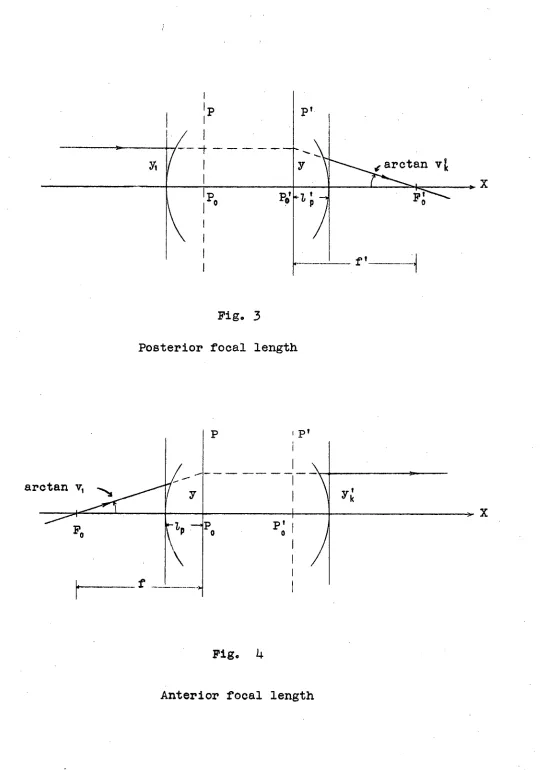
is unity. Let Ft! be the axial point of intersection in the image space of a paraxial ray incident on the system parallel With the axis. Then the posterior focal length, f l , of the system is defined as f t = P0!F4, (Fig.3). Likewise, if Po is a point on the axis in the object space such that paraxial rays from it are parallel to the axis in the image space, then the anterior focal length, f, is defined as f = POO, (Fig.4). Note that the lengths are measured from the principal planes.
As can be seen in Fig.
3
r •
By (2.6)
vpt y, +Vqi Vi
y, , since v, = 0 .
Thus
f' =
1/4 . (2.15)
For the anterior focal length, (Fig.4)
f = y/v, ,
Thus
8.
and (2.16) becomes
Y l k v (y' v' - y l v )/vA 1 qk pk A
N t v i yolk from (2,10).
Hence
N
- Ns /Ng vreik - ft (2.18)
The distance 7,1) of the first principal plane from the first surface is given by
= (11/Tig Vk )/vA . (2.19)
74, the distance of the rear principal plane from the last surface is given by
= (
4
k-
(2.20)Jberrat ion Coefficient
(a) In section 1, the aberration . of a ray in the jth image plane, E', was defined as
= h' (3.1 )
Thus H' E (3.2)
Multiplying throughout by N'vj, (the subscript "o" in this context denoting quantities associated with rays from the axial point of the object) we get
9
.If IA is the axial distance of the Oh image plane from the Oh surface, from(1,6)we get
ht = /Jvt - yl (3•4)
remembering the sign convention for h', Thus
Ntvjh' 11'14(14v' - 10)
N'vg(ni/v4Ovt yt] Nt (yJvt - vie)
which is the invariant X, by (2,9). Hence (3.3) becomes
(3.5)
Writing A for NvoH, and g for. Miroe
AA = Ag (3. 6)
Incidentally, since N'vjh is an invariant
N i vdh t Nivot hi (3.7)
t or h' = mh , where m =Nivo, /DIV0 ,
and is termed the paraxial magnification associated with the planes Fl and_
11.
The paraxial magnification associated with thefinal ideal image plane Fg is
10,
Now, the fth ideal image plane is also the Oth
object plane, hence
(3.9)
Also = NJ + i and v (Ii = v e thus
Now
A
el Sj 4.1 (3.10)
A
a"' ei E2 Z2
( I ) (
Ag 2 + • • •
A
0 • 0 ek +
— 4- i; from (3,10)
) (gi gk)
Agk . (3,11)
A
ef!
g
s
eI ""' a goo
However, e l E 0, thus, using (3,6)
A
ek AAi
1.1 — (3.12)
AA = Nev4H 1 Nvoll
and
= Z a V Y, from (1.4), thus
&A. = A[N(ve Y (3,13
Since Y,IT, depend on AA may be expanded as a power series
In Y1 ,V1 , Due to the rotational symmetry of the optical system,
if Y, are reversed in sign,
a
reverses its sign, andtherefore also must A4, Thus A4 must be a sequenced'
polynomials of odd degree in
/-1 ,21 .
Furthermore, AA tends tolimit, so that the series for AA does not contain linear terms.
Thus the expansion for AA can be written in the form
where
Co U g
_2 (fri,R) Y1 + g1p(v - 11 ) Vs ) nil v41i
n., v.0 v-
Ei = Y1 2 + 21 2 ,
111 = + Z1 W1,
v1 2
+ w1 2 •
(3.14)
(3.15)
For convenience, the early terms of the series (3.14) are written
AA = (aYi E 1 + tiVi Es + byi iii + _ TDVI _ _ _ 1 1 + cY1 4 1 + .c.;Vi 41 ) +
( si Yi Ei + ii _ .... - -. VI Ei -1- 82Y1E1r11 4- ii2V1EIT)I 4-
83 YI .. E 1 41 -4- T33 Vi E i I _ + 84 YI 11 i 4- E-54 VI rli 85111_ ... 1141 4-
i21-3 VI iti .1. s6 Yi 4; -F. I:14 V12 ) +
(t1 y, 1 1/14i ) 0(9)9
where 0(9) denotes terms of degree not less than9 in the
coordinates.
Writing
J-1
G 1.1,v Z (n) iu1 -110
(3.16)
and G(Wi = ,(n )
1-tv ep..v
and similarlyfbr the barred coefficients, (3.12) becomes
E g = n01 2 . (3.17)
11.0 v.0 gvk- gvk - 1
053
Z 2 (G (11)r Yi + 5 (11) 'V 6"N/it-ye
11.
12.
g
= (My, El + . ot! ) (silk yi
Ei + ...+ VI ) +(TA( pEt + Vid) + 0(9). (3.18)
The coefficients Gpvk(11)/' d (
p vk are called the (augmented) canonical aberration coefficients
or
order ,n of the system, and theg/
1;,)p g7A
are termed the contributions to these by the jthsurface. Gplds (n) pvj Gj are called the intermediate canonical aberration coefficients. Note that Gig, = .1 j11 = 0.
(b) AAj delJends linearly on ym , vm , by virtue of (3.13), (2.6). Thus the coefficients in (3.14) must depend linearly on ym , vm , so that
(n)
gin) p Yo + gin(o)) VO
- (0 -
= v p Yoi gril(0 V q v0 I (3.19)
Then the "p" aberration coefficients are
G 2 a (11) p.vpk 1.1"11Vp1
and the "q" aberration coefficients are
G
Wicik 1.1 -11vqi a
and similarly for the barred coefficients,
Thus '61 can be written as the sum of two series, one containing only "p" coefficients, and the other containing the "q" coefficients, in the following manner.
= (GI.L(vn)p' k + dp,(vn); k )C1 s Yot + 222(G
v q k V )t T)
p, (3.20)
13,
dloPpki AP k 64 - = A cjk
GPoi p k B pik 9 • • • (3.21)
The correspondence between the alphabetic symbols and the various values of g,v in the different orders is given in the following table.
Third order 01 v 00 10 11
n=1 A B C
10 11 20 21 22
82 S3 S4 SS S6
10 11 20 21 22 30 31 32 33
T2 T3 T4 Ts T6 T2 Te T9 T10
Fifth order 00 n= 2 Si Seventh order 00
n.3 Ti
4. "a" and "b" Aberration Coefficients
If the object tends to infinity, i.e. 1,01-00 then vm - O and (3.20) becomes
a =
zzz (G
(n)P 130 1-1 + J. )Vit-P" g-v v Ym1.1p - 1Vpk - (4.1)
NOW
Ng VA ell
Ni/§k(vjk Yol Vol )
Thus, omitting the subscripts and primes of the coefficients,
114.
where 11 = 1/tivA That is, only the p coefficients are re-
quired for the description of ei.
Consider a pencil of rays from an infinitely distant
object point in the tangential plane. Let this pencil make an
angle VI with the axis (VI = 0). Let p be the distance of the
paraxial entrance pupil from the pole of the first surface
(See M Section 33(a)). Then taking polar coordinates p ,O
in the first polar tangent plane, with the intersection point of
the principal ray as origin, Fig.5,
Yi =pVi + P cos° , Zi
•
P sine
W1 0 •
Equation (4.2) becomes
e = [ML 04)111k (pVI + P cose ) k v1 )
(P2 + 2pPVI C080 p2 )n41" (pV, + P cog/ )/1" v W4' v ] (4.3)
Considering third order terms only, and omitting primes and
subscripts from the notation of (3.21)
ei = 1.1./[A(pVi + Pcose) AV1 ][p2 N1 + 2pPcos0 p2 ]
[B(pVI + pose) + BV, ][pV, + Pcos0]
[C(pVi + pcose) av, + 0(5). (4.4)
Using the identity B =2A, from M 20.42,
CV = 111-AP3C086 4- [PA( 1 4- 2006e) 4. .A(2 4- C01320 )]P 2 V1
-
[3p2 A + 6pA 4 E 4. C] PVf cos°
›-
If, now, p = 0
= plAp 3 cose + A(2 + cos203)0V1 + (E+C)pVicose +
dv114. 0(5).
(4.6)
In this case, then, the p coefficients control the various well known types of aberrations in a simple manner. However, (4.6) results from the fact that the object is at infinity and the entrance pupil is at the first surface. In view of the
complexity of (4.5) or (3.20), it 4s obviously of advantage if expansions similar to (4.6) could be used even when vel 10, and p
((:).
By choosing a different set of initial coordinates to specify a ray this can be achieved. The new sets ofcoordinates are called "paracanonical coordinates". Para canonical coordinates Sy, gz, Ty, Tz, are defined in terms of the canonical coordinates by the following
Yi + Vi
TY, + , (4.7)
where a,
a,
T,
are disposable constants subject only, to the condition&
10.
(4.8)Since s, T are linearly dependent on Yi, yl l then any paraxial variable gi is related to the paraxial coordinates s, t by
where
P•aj S + (4.9)
= TY, + tiv,
16.
The gal gbj are the paracanonical paraxial coefficients, The
constants yaj , ybj, vaj, vbj are obtained in a similar manner to
their canonical counterparts, except that here the paraxial
tangential rays have as their initial data
"a-ray" , t
=0
,"b-ray" 0, t
=
1 .Thus, in terms of yl, vi, the starting data is, from (4.10)
"a-ray" yi = 't/g, vi -
"b-ray" Yi = Ei/g, vu t = a/g, (4.12)
whence, by using the recurrence relations (2.5) the values of
y, v at each surface will be Ya va for the a-ray and yb, Vb
for the b-ray.
The identity (2.10) becomes
Ya Vb Yb Va = Ni/N g. (4.13)
Thus an anteprime associated with a symbol is now to be regarded
as indicating division by NI /g instead of Ni as previously.
Since S, T are linearly dependent on Y1, Vi, (3.14)
can be written
00 fl
r n -11.„11- vy v
(4.14)
g t
n.I . .o V4V — —
0-
•••
■
and similarly for C. Here
s
y
2 4.T I = Sy Ty + Sz Tz • 41 = Ty 2 Tz 2
(3.20) now becomes
gg = Z2Z(G (M1 ' S d (m' T)61-141-v eso + ilvak - Pak
S + d (r
°1
TX vetotlybk Ilvbk
It is worthwhile noticing here that S, T, so,
(4.15)
to have no surface subscripts since they are defined only at the first surface, see (4,7), that is, there are no variables SbTi,s0,to
A particular Bet of paracanonical coordinates, OT
coordinates, are defined as follows. Let the principal ray of a pencil intersect the first polar tangent plane in a point whose coordinates are Y. Then Sy, Sz are defined as the y, z coordinates of the intersection of any ray of the pencil in this plane, taking YE as origin. Ty = HO T2 =
where /0, is the axial distance of the object plane from the first surface, see Fig.6. Thus, for these coordinates
0 = 101 (!,m p) 9 3= -13109 401
1/7Joi ,
1 .
From (4.10)
to = Yol + '7c" vo
(4.16)
18.
to = Yo +
0 . (4.17)
Thus the term involving to in (4.15) is zero and does not appear in the description of the aberrations in this coordinate system, that is, only the "a" coefficients are required. Changing the polar coordinates,
Sy = P OOSO p sine
Ty = =
R
say, Tz = • 0,so that p does not appear explicitly. Then taking only 3rd order terms and omitting primes and subscript k from the
coefficients, (4.15) becomes , taking si o for example
= [ Az P 3 0 Se + Ao ( 2 + c 0820 )P 2
(fa -I- 08,)Pre COSe # 8a1?
I
4- 0(5), (4.18)where 4 = 1/Ngvoic .
sg is now described only by the a coefficients, and the form of the expansion is independent of the value of 'Lot
19
This simplification of the form of expressions which arises from the
use of paracanonical coordinates is further demonstrated in the
following example,
From (3.7)
= m0 hi
= Ni vos hs vtik
= Ni Vs (I 01 "" p)/Ni (viik 7, et v4k ) , (4019)
where Vs refers to the principal ray.
The relation between the canonical and paracanonical
coefficients is given by
g pj = Oil, a + bj •
qj °P'ai T-1-Lbj (4.20)
With these and using OT coordinates it is easy to show that
(4•19) becomes
hi Ni T/Ni Vik • (4.21)
It has already been mentioned that to E 0 for OT
coordinates (4,17), which leads to considerable simplification in
the computations required to obtain the aberration coefficients.
This feature is common to all the sets of paracanonical
coordinates described in detail in M Section 13 (a), (b), (c)
and (d). These'coordinates also possess an additional feature,
namely that T(= -¶11 1 , M 13.71) is a constant for all rays that
issue from a particular object point. Thus in any pencil, the
only coordinates which vary are Sy,.Sz, in contrast with
canonical coordinates, in which, for a near point object, Ys, Zs,
20.
advantage when spot diagrams are to be computed.
OT coordinates, in particular, have further advantages over the other paracanonical coordinates. Firstly, they will apply when the object is at infinity, in which case T =
Secondly, g 1, and thus the factor NI/g is usually unity since most optical systems considered work in air. This means that the anteprimes which occur in the iteration formulae (see Section 5) may be omitted during computation of the coefficients. If NI
is not unity, say in an oil-immersion lens, then it can be made unity by multiplying all refractive indices by 1", the image forming properties of the optical system being unchanged by this process.
In view of (2.6), (4. 10); (3.14), (4014);and (2.14), (4.13), it is obvious that the derivation of the formulae for calculating aberration coefficients using either canonical or
paracanonical coordinates will be formally identical. Consequently, to avoid a multiplicity of symbols, canonical symbols will be
used almost entirely in the following work. If paracanonical coordinates are being considered, then, of course
Yi stands tor S VI stands for T ,
stands for (Sy 2 + Sz 2 ), it stands for (Sy Ty 4-
4t stands for (Ty 2 T2 2 ), (4.22)
the subscripts p, q are to be replaced by a, b, and the ante-primes will mean division by NI /g. It is worthwhile here to repeat that S, T are coordinates defined at the first surface only that is, there are no variables SLTj.
21,
5,
Calculation of Aberration Coefficients(a) Iteration
The formulae for calculating the aberration coefficients
are obtained by iterative processes. To demonstrate this
process two examples will be used. The first of these indicates
the basic method of the process. The second example is a
simplification of the process as carried out in M, so that by an
extension to a number of quantities, equations of the type M 11.3
can be obtained. This example also introduces the idea of
"pseudo—expansion" and "intrinsic coefficients",
Example 1
Suppose that x is some function f(t) of t, and that
x and t are related by the equation
0
X2 X 4- t •
(5.1)
We shall assume that f(t) is a, power series in ascending powers
of t, and is valid for all values of x. Suppose also that as
x 0, t-. 0. From this we can deduce that there are no
constant terms in f(t),
Rewriting (5.1), we get
t + 2. (5.2)
Then, as x becomes small, to a first approximation
= t, (5.3)
Substituting (5.3) in (5,2), one obtains
22,
thus we have a better approximation of f(t). Reinserting (5.4) in (5,2),
= t + (t + t2 ) 2
t + t2 2t3 +0(4) (5.5)
By continuing this process of substitution, the series for f(t) can be determined. This process, by which more accurate
approximations to the series for x are obtained by successive back substitution is called iteration. Iteration will only work when, as a result of resubstitution, the new terms generated are
of higher order than those that existed before substitution. For example, suppose that 1 as t in con- junction with (5.1). Then to a first approximation
(5. 6)
= 1 4- t .
Substituting (5.6) in (5.2), we get
t (1 ÷ t) 2 = 1 3t + t2 .
Resubstitution of (5.7) in (5.2) gives
+ 7t + 9t2 + 6t3 + 0 (4).
(5.7)
5.8)
It will be noticed that the coefficients of t o , tl , t2 0 .. will now vary at each iterative step so that the process does not converge to a fixed series for x. This is a result of the constant term in (5.6), (5.7), (5.8),
2
3,
= t
+ t2 + 2t3 + 5t4 + 0(5) . (5.9)Suppose we write the series for x as
ao 4. as t + at2 + at3 + a. t4 + (5.10)
Now, since x 0 as t --. 0,
0, (5.11)
so that (5.10) can now be written
as t + a2 .t2 + a3t3 + a. t4 + 0(5). (5.12)
Substituting (5.12) in (5.2), (5.2) becomes
= t t a2 t2 + a3 t3 .2 • 0 )
= t + a t2 + 2as 82 t5 + (2a, a3 + a )t4 + 0(5). (5.13)
Comparing coefficients between (5.12) and (5.13), one finds that
as 1
2
8.2 as
a3 = 2a1 a2 2
84 (28,e,3 + (5011+)
thus (5,12) can be written
X t + t2 + 2t3 + 5t4 + 0 ( 5 ) (5.15)
which is identical with (5.9). Thus the "complete" series for x
24.
only give correct results in those cases where direct iteration
produces a unique series for x (in contrast with (5.7), (5.8)).
It will be noticed in (5.14) that the coefficient a o is
expressed as some combination of coefficients of terms of degree
lower than n, Thus having found the first coefficient
explicitly, the rest can be easily computed,
Example
Consider the series for AA, (3.14), but for the sake of
simplicity suppose that there is only one variable Y, so that
now
n.I g ( " ) Yia (5.16)
where CI
Y.
As before, we shall write the first three terms of (5,16)
explicitly as
that is,
(I)
aY, CI + sYi Ci + tYiCi
a, g (2) g 00
+ 0(9)
t.
9 (5.17)
Now, at any surface
= f(Yi), cf(3.1). (5.18)
Suppose that
j- 1
YJ = rc(Y, + Z (5.19)
2
5.
constitution of the optical system.
J-I
Let the series for Z AAi be written
J-I
AjYii +
SOW + TjYiti + 0(9), (5.20)
where
Since A is an optical invariant when Y becomes small, to a
first approximation
Yi = ky,
•
(5.21)Inserting (5,21) in (5,18), AAj = f(YI) is a first
approximation to AAj o Knowing the function facY,), a series
for AAj in terms of Yi can be formed 'similar to 5,17),
namely
AJ = gi(n) yi
4. jYii
'DJ
YI VII 0(9) (5.22)This series is not the one required since the term kZ AAi
has been '.omitted from the expression for Y (5.19). The series
(5.22) is caned the "pseudo—expansion" of AAj. The coefficients
of this series j,
j, 'W..
depend only onR,
and hence they26.
reason they are called "intrinsic coefficients".
Now (5.22) gives us hAi correct to the first order, cf (5.3), hence (5.20) is also known correct to the first order. Thus the substitution of
CM
4. 2 &Ai) for M in (5.22) will give AAj correct to the second order, since MA is of 0(3) and will not affect the terms already present in (5.22), cf (5.4). Thus we have ZAA correct to the second order, and the process of reslibstitution in (5.22) can be continued, and so the series for AAA can be obtained.As before, the process can be condensed by writing the correct series for Aki as
AAi ej.M EI + Si Yi Ei + ti Ei + 0(9) (5.23)
and also
Aj Ei + Sj + Tj Yi + 0(9),
(5.24) J- 1
then, by replacing M in (5022) by
CM
2aM) and comparing coefficients between the resultant series and (5.23), the formulae for obtaining the higher order coefficients can be read offdirectly. (By way of comparison., in example 1, x = t, (5.3), corresponds to the pseudo-expansion of AAj, t corresponds to
f(kY, ), x to AAj and x2 in (5,2) corresponds to
_-
27.
+ AY, E + SY, EI + TY, Et +.. ) (E, + 2Y, [AY, E, + Sy, Ei + . . + + [AY, E + SY, El + ) 2 )
s (y1 + AY, c + sY, + ) (1 + 2Y1 [AY, cs + +[AYI c I + •. 32 )2
t ( -
Y1 + ) (EI +•) 3 + 0(9)
= a (Y, AY1 SY1 it (E 1 4- 2AEi + 2SEi + + A2 i + )
(Y, + AY, E +•) + LtAZi • •
t (Y1 + 4).* ) (Et + ..• ) 0(9) • (5.25)
Comparing coefficients between (5,23) and (5.25), we get from the coefficient of 'Yis a = a , (5.26)
Ei s = s + (2A + A)a
= s 3aA, (5.27) Y, t = t + s(I4A + A)
a(2 S + A2 +2A2 + S) t + 5sA + 3a(S+A2 ).
(5.28
(5.26), (5.27), (5.28) are the iteration formulae which enable' the contributions a, s t to the aberration coefficients i (5.23),at any surface to be obtained from the intrinsic coefficients of the surface and the sum of the contributions over the previous
surfaces (5. 24).
For example, at the first surface
Al Si = Ti = 0,
28.
hence, from (5.26), (5.27), (5.28) one finds that
al =
SI = Si
ti = ti •
Now
A2 al
S2 Si
.T2 = ti,
so that at the second surface
a2 a2
82 = 82 3a2 a,
t2 =-. t2 + 582 al + 3a2 (s, + a ).
Then
Eli + a2
S3 Si +$2
and the coefficients az', s3, ta can be found.
In this manner the contributions to the final aberration
coefficients by each surface are found. Notice here that any
inaccuracy in the value of AAj and hence of el/ comes, not
from the coefficients, which are exact, but from the fact that we
terminate the infinite series for LA1(eg) without regard to the
remaining terms,
In M, iteration is carried out with four variables at
each surface. namely Yj, Zj, Vj, Wj, and corresponding to these,
relations between these, equivalent to (5.19) are, from M 9.3,4,
29.
= YPJ + yj + Yqj (VI + Ovi )
(5.29)
Vi Vpj Crt + yj + Vqj (VI + 8 %1 )
where
•
i'.1 ,
6 Yi = - 2 A Il v.: • , -
J- 1 %
Ovj = + I A AO
1 ;• (note anteprimes). (5.30)
Each of the relations (5.30) represents two relations, e.g.
j -
- A Ayqi
i . 1
- 2 A A zq i
9
( 5 3 1 )
L4q is, of course. given by an expression of the form (3.14),
but containing only q coefficients,(3.19),1.e. ym = 0, and
similarly for A4p.
If now "increments" §y, v are neglected in (5.29)
Yj Yp j Yt + Yqj V1,
Vj= vpi Y, + Vqj Yl
(5.32)
then using (5,32) in (3.13) or an equivalent expression, the
pseudo-expansion of AA will be obtained, see M 10.1. If then
in the pseudo-expansion Y1, 1T, are replaced by + 6 y),
Ov) the iteration formulae ?Jr 10.2, 11.3, 81,3 can be
obtained. The intermediate p and q coefficients in M11.3, 81.3
30.
Intrinsic Coefficients
The straightforward method of calculating the intrinsic
coefficients is to expand the expression (3.13) for AA as a power
series in Yj, V), cj, nj, 4j, then convert this series to one in
Y1, IT,, CI, lii, 41 by means of (5,32), whence the coefficients of
the resultant series are the intrinsic coefficients. However, it
proves more convenient to first factorize (3.13) and then expand
one of the factors as a power series. Multiplying the coefficients
of this series by the appropriate factor then gives the required
coefficients.
Now
AA = (6.1)
from M14.5, where E = NrI and J is given by M 15.1
namely J = u4($ - 1) - vi(T - 1). (6.2)
Taking first order terms only,
= E j(I)
• - int int
= eq , (6.))
where ep = Nrip , eq = Nriq, Here E has already been
expressed in ,terms of Y1, Vi, by means of (5.32) (i.e. (5.29)
neglecting increments).
Now, for example, a is the coefficient of Y1E,,
that is the product, ep.(coeff, of Cs in Ji(p. (6.4)
Without going through the algebra, M 17.4 gives the expression
for J (1) ,
31.
where the y's are given by M 17.1, namely
Yi = k + 1)c2 - k2 crt + ik(k + 1 )4
T2= .4(k - 1 ) 2 C2 k (k 1 )01 4- k2 (6.6)
where k = NAV. Since uo. = Ave = v(1 — ve, (6.5) becomes
J(I) = (vrj ve )y, + (6,
7)
Now, in (6.6)
E = -il + z1
YjVj + Zgli
4 .
therefore, expressing T1, in terms of Yi Vi by means of (5.32), we get
= Y2pi + 2Yp + y2qi
Yp Vp + ( Yp Vq + Yq Vp )111 Yq Vq4
4 2Vp Vq1 + Vit4 (6.8)
Thus the coefficient of i in y, is
(k2 k + 1 )c2 — 2k2c ypvp k(k:f1)14 ( 6 .9)
Now, it can easily be shown that
32,,
and
ip k(C 2 ST2p 2cypvp vt) ) (6.11)
From (6,10), (6,11) it will be seen that (6,9) can be written
:(ip ill .1. ) . (6,12)
Similarly, the coefficient of gi in y2 is
4-[-(k - 1) 2 02 34 2k(k - 1 )cyp vp + (1 - k2 )vP
= ilv2p (k2 - 2k + 1)c2 + 2k(1 - k)cyp + k2 v2p I
= i(v2p y2) • (6,13)
Thus, from (6.4). (6.7), (6.12). (6,13)
a = Nrip [ (via — vo) (ipii + vP 2 ) + va(v — VIP )]
= Nrip [i (v0- Vp )Yol +(V4—rq )Voi ip + VTp Yeti +Vs; re, I
Ivf) — v0 2 1 .
Now, ap is the coefficient of yol YII (aq is the coefficient of
Vol Yi ), thus
gitP= iNrip (VO Vp )(1p1 4. + VP (4) VIP )
iNrip (ip ) [ (ip (vp + vpi )
Since the barred coefficients are associated with V,, then
q are l from (6.3), eq. (coeff. of yo' Cs , ViCI in J
In this manner, the coefficients in M 24.2, 24,3, 218,7 are
obtained,
3
4.
PART II - Computer and Programmes
7. Computer Description
The computer used for this work is the English Electric
DEUCE housed at the University of New South Wales, Sydney. The
machine operates entirely in the serial mode on 32 bit numbers.
The high speed store consists of acoustic mercury delay lines of
various lengths, the smallest containing one word (32 bits) and
the largest containing 32 words. In detail, the high speed
storage is as follows:
Four single word stores.
Three double word stores.
Two four word stores.
Twelve 32 word stores.
the total high speed storage being 402 words. The slow speed backing store is a magnetic drum containing 8192 words arranged in
256 tracks of 32 words each. The drum has separate read and write
heads on opposite sides of the drum, each bank consisting of 16 heads
which can be located vertically in any one of 16 positions, thus
covering the entire 256 tracks. Information is read to or from the
drum via one of the 32 word delay lines in blocks of 32 words. Drum
transfers and head shifts proceed automatically once they are set up
and do not interfere with the normal operation of the machine,
provided that access to the transfer delay line is not required.
The transfer of a block of words from the drum takes about 13 m secs,
and a head shift about 50 m secs. The digit frequency of the
machine is 1 megacycle; thus a single word store containing 32 bits
needs 32 gsecs to deliver one complete word at its output. Hence
the basic timing of the machine is tied to this time which is called
a "minor cycle" abreviated m.c. The circulation time of a 32 word
store is 32 m.c., that is, the same word is presented at the output
every 1024 gsees (approximately I msec). This interval of time
is termed a "major cycle", abreviated M.o. The 32 word stores
are termed "delay lines". Thus the machine contains 12 delay lines,
numbered for addressing purposes from 1 to 12. The remaining shorter
delay lines are simply designated as single, double, or quadruple stores.
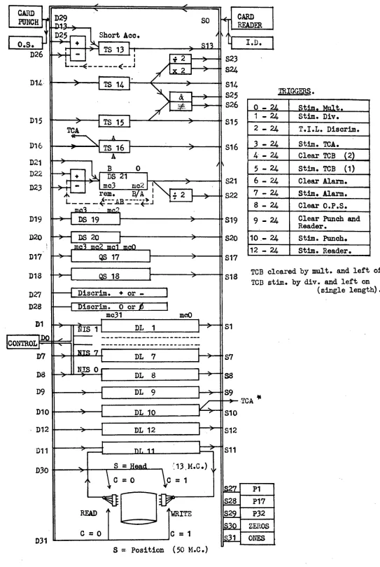
It is a feature of this machine that arithmetic processes
35.
addressed determines the type of arithmetic operation performed.
The inputs and outputs of all high speed stores are connected via
numbered gates to a common line called the "main highway". The
output gates are called "source gates" or more simply "sources",
and the input gates are called "destinations". Thus the basic
instruction of the machine contains two addresses, one for the
source and one for the destination. It will be realized that if
the input and output of any one store are connected, the word
contained in the store will circulate indefinitely. A
non-destructive read out is obtained simply by tapping this circulation
path. The read in of a new word ill obtained by breaking the
circulation path and connecting the input to the main highway, the
circulation path being restored as soon as the last digit is read
in to retain the word in the store (the connection to the main
highway being opened at the same time of course).
Owing to the fact that words in the delay lines appear
sequentially at the source gate, the instruction word contains an
extra number, called the wait number, which determines at what m.c.
the instruction will be obeyed. Since the circulation time of the
longest store is 32 numbers in the range 0-31 are sufficient
for this purpose. Zero time is usually taken to be the m.c, in
which the first instruction/word enters a delay line from the card
reader at initial input. Thus words in a delay line are denoted
by 0, 1„.. 31, "0" referring to the first word read into the
machine in any particular programme. Programme instructions/words are read into the delay lines from cards in binary form, and the
input programme is so arranged that, having read the first word into the first delay line, the first word read into any other delay line
also has a wait number of 0 associated with it, Thus the
sub-sequent location of words in any delay line is known,
The control section of the machine which interprets
Instructions and sets up the required gates has direct access to
any of the first eight delay lines, However, any particular
instruction in a delay line is not accessible to control except at•
the output. Thus an additional number is required in the
instruction word which indicates to the control when the required next instruction is accessible, called a timing number. As with
the wait number, the timing number is in the range 0-31„ The
particular delay line is also specified, of course, and the numbers
here are in the range 0-7, 0 referring to delay line 8. Finally,
36,
transfer the 32 words of one delay line to another with one
instruction. With one instruction transfers can be performed for from 1-32 m.c. The duration of a transfer is determined by the
difference between the wait and timing numbers, which, in the case of long transfers (more than one word) restricts the location of the next instruction. The instruction word is as follows:
Digit position in word Function
1 (least significant digit) Not , used
2 Next instruction source, i.e.
3 Delay line 0-7
4 5 6
7 Source gate number
8 Range 0-31
9 10 11
12 Destination gate number
13 Range 0-31
14 .
15
16 Long or short transfers
17
18 Wait number, referred to time
19 instruction enters control
20
21 22
23
24 Special use
25 26 27
28 Timing number, referred to time
29 instruction enter control
30
• 31 Not used
37.
It will be noticed in the preceeding table that the wait
and timing numbers refer to the time that the instruction containing
them enters control as their time reference, As mentioned before,
the machine keeps track of m.c, only, hence it does not know which
m.c, of a delay line the programmer has referred to as 0. Thus it
Is the programmer's job to keep track of the location of words at any
subsequent time. For instance, if a word with the m.c. number 6
enters control, and a transfer of word number 27 is required, then the wait number in the instruction will be 19 since a minimum 2 m.c.
are required to obey an instruction - one m.c, to read in the
instruction and one m.c, to set up the gates. Then, after waiting
19 m.o. from the set up the gates are opened and word 27
enters the main highway. The minimum time to Obey any instruction
Is 2 m.c, e.g. an instruction entering control in m,c. 11 can, at
best, be obeyed in m.c. 13, the wait number for this being 0. Thus the sequence of events here are, instruction enters control
in m.c. 11, gates set up in m o c e 12, no wait so obeyed in m.o. 13.
The location of words by the programmer is facilitated by arranging
the coding sheets in columns of 32 words representing the state of
a delay line at m o o. times 0, 32, 64, 96, Apart from the
direct access to delay lines 1-8, control can accept instructions
from any other high speed storage location, but this requires a
separate instruction, this being considered as simply a normal
transfer between stores. In this event, the next-instruction-
source number of the instruction is ignored by control, since, when
the transfer is complete, control has its next instruction.
The DEUCE machine has no indexing registers, but digits
22-25 in the instruction word may be used for this purpose, Digits
in these locations are always ignored by control. However, by
placing an instruction in one of the stores that has adding
facili-ties, digits may be added into these locations each time the
. instruction is obeyed during a repetitive loop. Eventually, these
will overflow into position 26, that is, the timing number will be Increased by 1 and a different instruction from the normal one of
the loop will enter control and thus exit can be made from the
loop. A particular use of this facility is when numbers are being
transferred successively from a delay line by increasing the wait
number each time around the loop, If the digits 22-25 are all
ones, when the wait number exceeds 31, the overflow will be carrie4
right through to the timing number, giving exit to the loop.
As mentioned before, the minimum time to obey an
38.
able to transfer words for more than 1 m.c, with one instruction, it is possible to add/subtract the entire contents of a delay line (32 words) in 33 m.o. For example,words sent to destination 25 are added to the contents of the single word store 13 (see Fig. 7). Thus; if 13 is originally clear, then a long transfer of 32 words from delay line 1 0 say, to destination 25 will produce in 13 the sum of the contents of delay line 1 after 33 m.o, from the time the instruction entered control. It will be seen in Pig 7, the schematic diagram for DEUCE that double word store 21 also has adding/subtracting facilities.
However, this store is not generally used for sequential adding, these facilities are to allow arithmetic operations on the results of
multiplication/division, which appear in this store, Multiplication/ division are carried out on numbers stored in 16, 21, and are
Initiated by "trigger" instructions, Shift facilities are associated with store 14, the digits appearing at source 23 are those of 14
shifted down one place, the digits from 24 are those of 14 shifted up one place. Multiple shifts can be simply obtained by a single instruction of the type 23-14 for any number of m.c, up to 32, whence the digits of 14 will be shifted as many places as the number of m.c, of the transfer.
Logical operations are performed between the content's of stores 14, 15 by sources 25, 26. Discrimination on sign or magni-tude of a number are performed by destinations 27, 28 respectively
(negative numbers are two's compliment). If a positive number is sent to destination 27, then the next instruction as indicated by '
the timing number is taken into control; if the number sent to 27 is negative, then the timing number is increased by 1, causing control to take a different instruction,
It is possible to alter the m.c, numbers of words in a long delay line by using delay line 10 and store 16. By initiating a special trigger (T.C.A.) the output of 10 is connected to the input
of 16, Then a long transfer for 32 m ac, between source 16 and destination 10 will result in the words in 10 being shifted down one m.0,0 i.e. word number 0 becomes word number 1 00090
word number 31 becomes word number 0 0
Sources27-31 are constants, 28 generates wait numbers and Is used mainly for instruction modification. Source 30 is used to clear stores. Source 31 is mainly used in logical operations.