Selection of optimum machine parameters for maximum production rate (minimum time) criteria in single pass turning operations

Parameters For Maximum Production

Rate (Minimum Time) Criteria In

Single Pass Turning Operations

by

Colin Braganza

(Bachelor of Engineering)

Submitted in fulfilment of the requirements for

the degree of Master of Technology

I would like to thank my supervisor Dr Vishy Karri for all his help, time and support in completing this thesis.

Thanks also to all the postgrads who helped throughout the year, especially Michael Koutsoukis for all his time and tips.

I would also like to sincerely thank and dedicate this work to my parents and sister for their encouragement, help and moral support that they have given me

Abstract

The purpose of this work is to investigate and develop optimization techniques

used for single pass turning operations on CNC machine lathes. The scope of this

work is limited to the Maximum Production Rate Criterion (Minimum Time

Criterion) for two machining variables, feed rate

and machining speed (v).

Further, a comparison of three methods of finding the optimum solution will be

made. The three methods used are:

1. A combined mathematical and graphical based optimisation technique

2. Real time simulated optimization on a CNC lathe

3. Neural networks to obtain optimum cutting conditions

The comparison of optimum time with limited constraints using mathematical

models and that of more optimised trends in CNC lathes give a better

understanding of the accuracy of modern machine tools and limitations of models

with limited constraints. Further, the neural network is also used as a decision

making tool in determining the optimum cutting conditions. It is hoped that the

neural network estimation of optimum cutting conditions are of reliable

Page

Introduction 1

Chapter 1: Literature Review 4

1.1 Optimisation 9

1.2 Technological Constraints 10

1.2.1 Feed and Speed Constraints 11

1.2.2 Three Force Constraints 11

1.3 Optimisation Criteria 13

1.3.1(a) The Minimum Time Per Component

(or Maximum Production Rate) Criteria 14 1.3.1(b)The Minimum Cost Per Component

Criteria 14

1.3.1(c) The Maximum Profit Rate Criteria 15

1.4 Tool-Life Equations 19

1.5 Optimisation Techniques 24

1.6 Classical Modelling of Turning Operations 25 1.6.1 Single Pass Turning Without Constraints 26 1.6.2 Single Pass turning With Constraints 32 1.6.3 Multi-pass Turning Without Constraints 35 1.6.4 Multi-pass Turning With Constraints 37

1.6.4.1 Example of a Strategy Used For The Optimisation of Constrained Multi-Pass

Turning Operations 37

1.7 Artificial Neural Networks 40

1.8 Concluding Remarks 50

Chapter 2: Computer Integrated Manufacturing (CIM) 53

2.1.1 Benefits of CAPP 54

2.1.2 Types of CAPP 54

2.1.2.1 Example of a Generative CAPP System 57

2.1.3 State of The Art CAPP Systems 57

2.2 Concluding Remarks 62

Chapter 3:Unconstrained and Constrained Optimisation For Single

Pass Rough Turning Operations 64

3.1 Unconstrained Optimisation 65

3.2 Constrained Optimisation 72

3.3 Application of Mathematical Model 74

3.4 Results of Mathematical Model 76

Contents

Chapter 4: Real Time Optimisation On CNC Lathe 82

4.1 Machine Tool and Tool-Workpiece Specifications 83 4.2 Description of Experimental Method 84

4.3 Discussion of Results 90

4.4 Concluding Remarks 92

Final Concluding Remarks 93

Future Work 95

References APPENDICES

Appendix 1 - Results of Mathematical Model (idealised optimisation) and Time Trials on CNC machine

Appendix 2 - Turning Operation Simulation Program Listing

Metal machining is a process which has been in use since ancient times. In more

recent times from about 1760 to 1860 there were many developments in machine

tools in England during the period of the great industrial revolution where

manufacturing techniques were needed to make components to an accuracy

formerly not attainable.

Machining processes have developed to a very refined stage in the manufacturing

industry today and its importance can in no way be underestimated. The

machining process is probably the most important method by which metals and

other materials are transformed into many of todays essential commodities. The

importance and wide use of turning processes today represents a significant

proportion of all machining operations. Hence, investigations for improving the

efficiency and effectiveness of machining operations is of great value in a very

competitive economic environment.

The need for reliable performance estimates is paramount especially from an

economical point of view. The advent of CNC/NC machines in manufacturing

has meant that time spent on actual machining components has significantly

increased from less than 6% of the total available production time for

Introduction

machine tools [1]. With such a large increase in actual machining time the need to

further improve and optimise machining times and costs becomes increasingly

more important in modern manufacturing industry.

The selection of machining conditions such as feed and speed have traditionally

relied on the experience of machine operators and on handbook recommendations

which are known to be

solutions but not the

solution. In recent

years attempts as evidence is seen in the literature review to develop computer

software to determine optimum. An in-depth study of a complex computer-aided

optimisation analysis and strategies for multiple constraint turning operations by a

researcher [4] at the University of Melbourne has recently been carried out

successfully. With the use of mathematical and graphical analysis detailed flow

charts were drawn and implemented to determine global constrained optimum

cutting conditions with given performance criteria. This information could in turn

be integrated into systems such as aided drawing (CAD) and

computer-aided manufacturing (CAM) to result in a fully automatic manufacturing process

incorporating optimisation conditions.

The optimization analysis for machining conditions carried out at the University

of Melbourne proved to be surprisingly difficult, requiring intricate mathematical

analysis and computer aided optimization strategies, which depend significantly

on the mathematical functions and quantitatively reliable predications of machine

performance characteristics, detailed specifications of machine tools, cutting tools

As materials improve with respect to cutting tools and workpiece materials, the

availability and acquisition of empirically determined tool-life equations and

related constant values for different tool-work combinations is difficult.

This work is aimed at studying and developing an optimisation technique for

single pass turning operations to determine the optimum machine cutting

condition for several tool-work combinations. The optimisation is based on the

maximum production rate (minimum time per component) criteria and

incorporates limited constraints such as the machine cutting speed and feed.

Tool-workpiece combinations are limited to carbide tools only due to restrictions in the

Chapter 1

Literature Survey

In todays highly industrialised and mechanised society, we are surrounded by

many mechanical marvels. Technical advances have come so far in recent years

that in less than a century humankind has learned to fly, explored the deepest

ocean and begun the exploration of space. Such technical achievements would not

have been possible had human beings not learned to extract metals from the Earth

and then shape them into useful products.

Many methods have been and are being used today to shape metals. However,

only a small number of these methods produce the wide variety of items as do the

processes of machining. In fact, machining is probably the most important

method by which metals and other materials are transformed into the many

products which are essential in todays high tech. society. This is based on the fact

that some machining is involved in the production of almost any item one can

think of. Even where machining is not directly involved, it is virtually always a

necessary process in making the dies or fixtures used in the production operations.

Machining is basically a process of shaping materials using a variety of cutting

tools. The material is shaved away in small pieces or chips (in one or more

In the last decade high precision machine tools have been combined with

electronics and advancing computer technology which has enabled modern

manufacturing to be computer controlled. The latter has led the way towards

programmable automation and the field of computer based manufacturing systems

such as computer integrated manufacturing (CIM), computer aided process

planning (CAPP), flexible manufacturing systems (FMS), computer process

control, computer aided handling and storage systems and computer networks for

manufacturing.

Consumers today are better educated about technology and its limits. Their

expectations (in terms of better value for money) of manufactured products have

also increased. This demand for a better product by the consumer has forced the

manufacturer to make products which are better designed. To the manufacturer

this means that it is not only sufficient to design a product that satisfies its

functional requirements (suitability for intended function, durability, and

aesthetical appearance), but to also manufacture it easily and as cheaply as

possible.

Auditing is one of the functions of the production activity and it is aimed at

checking the designs from a manufacturing point of view. It is a very necessary

function that enables the manufacturing department to design, select and/or

provide the processes, operation sequence, tooling etc. to enable the product to be

designed. The manufacturing department has various other responsibilities which

include the designing of manufacturing systems, quality management systems,

Chapter 1 - Literature Survey

Evidently, a strong link exists between design and manufacturing requiring full

cooperation between these two functions. The tendency today is to integrate the

functional design and the design for manufacture at the early stages of the design

process to prevent problems and extra costs at the manufacturing stage.

Sometimes, the design of a product is reconsidered or even changed completely

without altering the intended function. This process is termed "Value

Engineering".

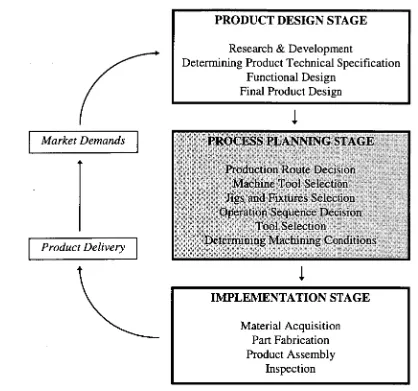
Figure 1.1 gives a global view of the steps that are necessary in producing a

product. The production cycle basically goes through three stages which are, the

product design stage, the process planning stage and the implementation stage.

In particular, the process planning stage where functions such as production route

decisions, machine tool selection, operation sequence decisions, tool selection,

and determining machining conditions, has captured the interest of researchers in

machining. The principle objective of research is the reliable estimation of

performance characteristics such as the three force components, power,

component surface finish and dimensional accuracy for a wide spectrum of

practical machining operations involving numerous process variables.

It then becomes apparent that even a slight decrease in complexity or the number

of steps in machining, or even an increase in tool life would result in substantial

time, cost and/or material savings in each of the above stages in the production

cycle.

PROCESS PLANNING STAGE _{. .}

Production Route D ""

0

.1

M

g s

'a

n

'd

and

n

, Fe T

t

o

r e

l

s

S

‘

e'

Selection

'lectl'so in°n

Operation Sequence Decision

Tool Selection

Determining Machining Conditions

Market Demands

Product Delivery

PRODUCT DESIGN STAGE

Research & Development

Determining Product Technical Specification

Functional Design

Final Product Design

IMPLEMENTATION STAGE

Material Acquisition

Part Fabrication

Product Assembly

Inspection

Figure 1.1 -

Functions of integrated manufacturing systems (IMS).

interest and benefits. In recent years the benefits of this study and its applications

have been realised by manufacturing industries. From a global point of view these

benefits include

• Lower costs per component

• Higher volume economic production

• Decrease in waste material

Chapter 1 - Literature Survey

• Better product consistency • More efficient process planning • Better customer service

• Better quality control on processes • Decreased reliability on human operators

• Predictable tool replacement and machine service times

Traditionally, the values of process or machining variables such as feed, speed and depth of cut have been determined either by machine operators, based on their past experience, or by process/production planning engineers. The latter combine experience with handbook and tool manufacturer recommendations in arriving at detailed process plans including the selection of machining process variables such as machining speed and feed. However, both of these methods rely very much on personal experience and handbook recommendations which are known to be feasible but not the optimal solution.

The advent of CNC/NC machines in manufacturing has meant that time spent on actual machining components has significantly decreased from less than 6% of the total available production time for conventional manufacturing systems to well above 77% for modern CNC/NC machine tools [1]. It becomes even more evident then, that the need for optimising machine variables and process planning to improve production rates and component costs are necessary in todays highly competitive industrialised world.

Cutting

1.1 Optimisation

Optimisation is the process which seeks the best possible solution for a given

manufacturing criteria. For example, consider the different ways in which the part

shown in Figure 1.2 could be turned on a lathe.

Figure 1.2 - Different cutting paths that could be used to obtain the part shown.

One can easily see at least 10 different patterns of the various paths in which to

turn the stock material to obtain the finished product. Apart from these various

paths, one can then choose the magnitude of the several machine parameters such

as speed, feed and depth of cut. The combinations are numerous. However, only

a few of the many combinations available will be feasible solutions, and only one

of the feasible solutions will be the optimum solution.

Optimisation analysis of manufacturing has been studied since Gilbert's first

work, Economics of Machining [2] in 1950. He introduced 'the maximum

Chapter 1 - Literature Survey

machining speeds were analysed by developing mathematical models for a single

stage manufacturing.

Single pass turning operations are possible and feasible in many situations

depending on the limiting constraints, especially if the operation is restricted by

the highest feed [3]. In single pass turning operations only one pass by the cutting

tool is required to cut the stock material to the desired shape. However, it has

been shown [3,4] that single pass turning is not always optimum. The more likely

situation will be that the operation is subject to such practical constraints as

available power, surface finish, minimum tool life, maximum permissible feed,

and a range of allowable cutting speeds. In this latter case, two passes, or

sometimes even three passes, can be cheaper or take less production time.

1.2 Technological Constraints

Most of the reported work in economics of machining has been devoted to single

pass turning using Taylor-type tool-life equations. However, many of the earlier

researchers have not accounted for the technological constraints (such as the three

cutting force and power constraints, surface finish constraints, and availability of

machining performance and machine tool specification data) in the analysis. It is

quite evident that when constraints are included in the analysis, the optimal cutting

conditions selected will be different because of the constraint effect. In order to

apply optimisation results for turning operations directly to practical machining

operations, many technological constraints caused by machine tools and

1.2.1 Feed and Speed Constraints

Maximum and minimum feeds (fmAx and fmiN) and rotational speeds (NmAx and

NmiN) have to be determined in the design of a machine tool. The available

rotational speeds N and feeds f should be first satisfied when optimum cutting

conditions are selected. As shown in Figure 1.3, these constraints make up a

rectangular feasible area.

NA

Feed (f) ...

Feasible Area

NmIN NMA

Speed (N)

Figure 1.3 - Feasible area in the speed-feed domain.

While any combination of machine speed and feed is not possible on a

conventional machine tool (since these variables are controllable only in discrete

step) they are infinitely variable for the modern NC/CNC machine tools.

Therefore, during optimisation analysis, a continuous path can be plotted on the

f-N diagram enabling the optimum solution to be used in practice. Furthermore, the

optimum solution can be determined to a high degree of accuracy.

1.2.2 Three Force Constraints

In most turning operations, forces acting between the tool and workpiece can be

Chapter 1 - Literature Survey

thrust force (Fq) components (Figure 1.4) and are also important constraints when

arriving at the constrained optimum cutting conditions.

Figure 1.4 - Oblique cutting showing the three force components.

Excessive forces between the tool and workpiece are considered undesirable. The

machine tool will rapidly wear out or even damage if it is overloaded with work.

In addition, the toolholder and tool piece will give a maximum radial force limit,

the workpiece deflection will restrict the maximum power force and thrust force,

and the machine tool feed system rigidity will limit the maximum radial force [4].

However, it is known that the forces at the tool-work interface are affected by

many variables such as speed, feed, depth of cut, tool geometry, and the tool and

work materials. Thus, it is important that the cutting conditions selected will not

only satisfy the economic criteria but also the force constraints.

Other constraints used in previous studies include low power/limiting spindle

torque constraints, maximum power constraints, surface finish constraints,

threshold of dynamic machine stability constraints, tool life constraints, and chip

strategy increases significantly as more constraints are included in the

optimisation analysis.

In this work, only those constraints which impose limitations on the cutting

conditions such as machining speed and feed rate is considered in the analysis.

1.3 Optimisation Criteria

With regard to economics of manufacture, aspects such as the criterion for

optimisation and tool-life equations for machining will first have to be clearly

defined.

The criteria functions are of significant importance in studying the economics of

machining. The type of criteria objective functions chosen would influence the

optimum result. Numerous plausible criteria have been employed in the

economics of machining studies, ranging from purely technological criteria, such

as maximum material removal rate and the very popular maximum production

rate, to the more financial criteria, such as minimum cost per component,

maximum rate of return and maximum profit rate.

The most popular criterion employed in optimisation techniques previously

reported [5-24] have been based on the minimum time per component (or

maximum production rate) criteria, the minimum cost per component criteria, and

the maximum profit rate criteria.

Chapter 1 - Literature Survey

criteria:

This criteria maximises the amount of products produced in a unit time interval;

hence, it minimises the production time per unit piece. This criteria is adopted

when an increase in physical productivity or productive efficiency is desired,

neglecting the production cost needed and/or profit obtained and is

given by

t m

t = t_p t_m t_e = t_p t_m t_c—_T

where t = production time per unit piece

t = loading, unloading, idle set up time per component

tm = machining time per component

te = tool-replacement time

tc = time required to replace worn cutting tool with a new one

and T = tool life

1.3.1(b) The minimum cost per component criteria:

This criteria refers to producing a unit product at the least cost. The unit

production cost is given by

u

u

p

=Inc + ktp + (k, + km)tm + (kItc + tm (1.2)

where m = material cost

up = preparation (or set-up) cost

tie = tool-replacement cost

U, = tool cost

u, = overhead costs

kt = direct labour cost and overhead

km

and kt = cost of cutting edge

It is evident that the governing equations for these two criteria are mathematically

similar, and the optimisation strategies for selecting cutting conditions have been

shown to be the same [4]. However, practically it is more advantageous to

develop the solution strategy for the time per component objective function since

this equation is simpler to use since it only requires time data.

1.3.1(c) The maximum profit rate criteria:

This criteria maximises the profit in a given time interval. Okushima and Hitomi

[26] used a profit (Pr) objective function for producing N units in a constant time interval

Pr = (c-b)N-a (1.3)

where a = fixed cost

b = variable costs

and c = selling price per piece

In analysing the maximum profit rate (Pr) criterion, Wu and Ermer [26] also developed an equation based on Marginal analysis

Chapter 1 - Literature Survey

where R = total revenue per minute

and C = total cost per minute

Both the R and C terms are functions of the cutting speed. Arrnarego and Russel

[6] formulated the equation for the maximum profit rate criterion in terms of time

per component (t) and cost per component (u)

P — (I

—

t

(1.5)

where

income per component (excluding material cost)

A similar maximum profit rate criterion as given in equation.(1.3) was employed

by Boothroyd and Rusek [27]. They extended the optimisation analysis to allow

for the effects of worker incentive schemes and batch production on the

machining conditions. Although the three equations (1.3 - 1.5) were derived from

different principles, the resulting equations are mathematically similar. The profit

rate equations appear to be more complicated for use in mathematical analysis

than the production rate and cost per component equations. So Chitale

[28]

proposed a rate of return

as a new objective criterion for machining

optimisation analysis

I —u R-

tu

(1.6)

By comparison, this equation is even more complicated than those above because

The above three criteria are often used in optimisation analysis for single pass

turning. Armarego and Wong [29], Iwata et al. [30], KaIs and Hijink [31] have

extended the t and u equations to multi pass turning using the general form; ie for t

t =t +Itc.(14-4-mtt, s

where m = number of passes

tc, = cutting time for the ith pass

ts = tool reset time per pass

and t = tool-lifu using cutting conditions of the i th pass

and for u

,

÷z te

U = + Lte,(1+7j+nits] (1.8)

1=1

where X = labour cost for running the machine tool

If the profit rate equation (Pr) and the rate of return equation (R) criteria are formulated for multi-pass turning, they will lead to an equation with many terms

on both the numerator and denominator such that the mathematical analysis for

finding the optimum conditions will be even more complex than equation. (1.7)

and (1.8) [4]. Ghiassi el al. [32] and Malakoot et al. [33,34] optimised the three

objectives (minimising total cost, maximising production rate and maximising

quality of cut) subject to some constraints. But these were found to be more

complex [4].

i=1 ti

Chapter 1 - Literature Survey

Although a variety of plausible criteria which have been discussed above can be

used, the maximum production rate (minimum time per component) and

minimum cost per component have been found to be the most popular criteria. In

the economics of machine studies, the appropriate criterion to be used is

dependent on the management policy and ease of implementation [4]. While

higher management levels might place more emphasis on the maximum profit rate

or the maximum rate of return criteria to justify the company investment, those

closer to the manufacturing levels would usually prefer the maximum production

rate criteria to meet certain deadlines or to reduce the bottle-neck in production

lines. In a non-profit making organisation, the minimum cost per component

criterion could be more appropriate. If time is more important than cost or profit,

then the maximum production rate criterion should be used.

However, more attention has generally been placed on the problems of optimising

conditions than in detailed analysis of the best criterion to be used. This is

understandable in view of the difficulties in obtaining the necessary data or

equations for the tool-life, practical constraints and the development of

optimisation and experimental strategies. From the above survey, it is apparent

that tool-life is the central element in economic machining. An understanding of

the tool-life and the equations relating tool-life to the cutting conditions is

therefore essential in the study of economics of machining if mathematical

1.4 Tool-Life Equations

A tool's life can end by catastrophic failure of the cutting edge or by exceeding a

critical wear level. Exceeding the critical wear level does not, in itself, result in

immediate deterioration of the tool performance to the point of incurring

economic penalties as would the catastrophic failure of the tool. Cutting may still

be acceptable if the tool operates beyond its critical wear limit [4]. However, the

economic penalties due to the propagation of tool wear are shown up by altering

various process constraints such as deteriorating surface finish, increasing cutting

forces, and increasing deflections and vibrations [4].

Catastrophic tool failure analysis has focused on tool failure distribution

modelling and is primarily used to determine the optimal tool replacement interval

[35], however these studies do not incorporate the influence of cutting conditions.

Gradual wear tool failure is modelled as a function of the cutting conditions eg.

Taylor equation. Therefore, this kind of wear failure is used in the optimisation of

Chapter 1 - Literature Survey

been placed on the tool-life data and tool-life equations rather than on the tool

failure criteria and tool wear mechanisms.

Various forms of empirical tool-life have been developed [36-38] by curve fitting

experimental data obtained from tool-life investigations because of the absence of

reliable theoretical tool-life models for quantitative prediction purposes.

However, there have been considerable attempts to establish tool-life

relationships, and tool-life equations can be classified into two categories

• Taylor-type equations

• Non-Taylor type equations

Earlier on this century Taylor conducted some experimental tool-life tests for

single pass turning [39] and showed that the logarithmic tool-life (log(T)) is

linearly related to the logarithmic cutting speed (log(V)), Figure 1.5.

200

100

1

2

300

Tool Life, T

Figure 1.5 - The Taylor tool-life curve. It shows a linear relationship between

tool life and machining speed on a bilogarithmic graph.

These results lead to the tool-life equation

vT° 23=43

600

500

vTn =C _(1.9)

where v= machining speed

T = tool life

n =

and C = 1 min tool-life machine speed (constant)

This is the widely known Taylor's tool-life equation. After Taylor, other workers in the field developed tool-life equations similar to Taylor's equation. Taylor also proposed the idea of using speed vr for a fixed tool-life T in turning operations ie when cutting speed VT is used the tool-life will be T minutes. By adopting a standard test period of 20 minutes, Taylor gave the cutting speed equation

I-

[48dix j 132r]

(1.10)

where V20 = cutting speed for 20 minutes of the tool-life

= constant

r =

f = feed rate (inches/rev)

d = depth of cut (inches) 2.12

x= 0.4 + 5+32r

and y=—+0.06V32r + 2 0.8(32r)

Chapter 1 - Literature Survey

v

r

was used as a means of comparing the machinability of different materials. In

the later Taylor-type tool-life equations it is noted that the nose radius

(r)

was

introduced to the equations since the nose radii in early tools were larger and

hence less significant. Because of the complexity of equation 1.10, it was not

used in practical operations [4].

After Taylor's experimental studies on tool-life other workers [40-43] attempted

to follow this approach of first finding the effect of feed and depth of cut on

cutting speed for a fixed tool-life and then the effect of cutting speed on tool-life

for a given tool work combination and cutting conditions. The reported results

were generally similar to Taylor's although the effect of nose radius of the cutting

tool was omitted ie

where

, p and q are constants for the conditions tested.

Kronenberg [40] combined equations (1.9) and (1.11) into a single relationship

and proposed the "extended cutting speed rule" equation

C, ()

(1000A) z

(

1.

60

(1.12)

where

= tool-life constant

60C„;

n= y; n, — , n2 — (1.14)

g + z z — g K — z

5) (1000)Y

A = area of cut = df

and y, g,z = empirical exponents with z > g and (z + g) <1

Thus equation (1.12) is similar to the extended Taylor's tool-life equation quoted in many books [44-48]

T — (1.13)

V 'f n1dn2

Comparing equation (1.12) and (1.13) the following relationships can be shown which highlight the similarities between Taylor's tool-life equation and Kronenberg's tool-life equation

From the equations above, it can be concluded that tool-life is affected by the cutting speed (V), feed (f ) and depth of cut (d).

Extended Taylor-type tool-life equations of the form

T— v". f in'dn (1.15)

where C = tool-life constant for the Taylor-type tool-life equations T = tool-life

Chapter 1 - Literature Survey

d = depth of cut

n

o

=

mo = tool-life cutting feed exponent and n = tool-life depth of cut exponent

have been favoured in optimisation analysis and have progressed to an advanced practical stage - but at a slow rate. The reason for this advancement is that additional factors such as feed rate, depth of cut, and cutting tool radius have been introduced to Tailor's initial tool-life equation (1.9).

As can be appreciated, a large number of tests must be carried out at different cutting speeds in order to establish a Taylor line with any degree of confidence. With the addition of these new factors, the testing is significantly more laborious. Compared to non Taylor-type tool-life equations, 1Cronenberg [49] found that about 70-80% of commonly used tool-work material combinations could be represented by the popular Taylor-type tool-life equation. Other reasons for the popularity of Taylor-type tool-life equations are its mathematical simplicity, and tool-life data for the extended Taylor's equation can also be obtained in the literature [40] and machining handbooks [43,47,48].

1.5 Optimisation Techniques

decades quite successfully is the method of using classical mathematical calculus together with graphical representation in the cutting speed-feed domain to develop the optimisation analysis and is used in this work. There has also been a tendency to use numerical optimisation computer packages in attempting to arrive at required cutting conditions. However, numerical search techniques have the disadvantage of being unable to guarantee that a global optimum solution can be found since these techniques perform a pattern search with a random number generator as a starting point. The use of combined mathematical calculus and graphical representation of economic trends and constraints in the speed-feed domain has led to clearly defined constrained optimisation strategies with guarantied global optimum solutions. Other techniques include geometric programming and dynamic programming, but share the same disadvantage as numerical search techniques in that they do not guarantee a global optimum solution.

In the later part of this study artificial neural networks (neural nets) is used and so a brief treatment of artificial neural networks follows.

1.6 Classical Modelling of Turning Operations

Chapter 1 - Literature Survey

this field. As the focus is shifted from single pass to multi pass turning

operations, and as constraints are considered, the mathematics become more

complex and laborious. However, it is not the aim of this work to present the

more complex conditions of turning operations, especially multi pass turning

operations with constraints, but they are briefly looked at.

1.6.1 Single Pass Turning Without Constraints

Most of the reported work in economics of machining has been devoted to single

pass turning operations using Taylor-type tool-life equations [4]. Single pass

turning without constraints is the fundamental condition in turning operations.

Everything else is an extension of this condition. Some other workers have used

non-Taylor tool-life equations in their analysis but are not discussed in this work.

Hitomi [50] has shown the optimum machine speeds under the three evaluation

criteria for a fixed depth of cut and a fixed feed rate to be

1.

(v

i

):

vt - I- 1 -

In

I_( 1

7

1

1)

(1.16)

where

C

= one minute machining speed (constant)

n =

slope of Taylor tool-life curve (constant)

Chapter 1 - Literature Survey

=(-1)t,

where = time required to replace a worn cutting edge with a new one

2. The minimum cost machining speed (vc):

i

n

1 (ki + km )

vc=q 1 k t

--1

_{1 c t}

L n

where

lc

/

k

m

=

and

k

t

=

The minimum cost tool-life ( Te)

1

jk t +k

T

c 4n

1 i c

+k:

(1.18)

(1.19)

Using the partial derivatives

aciav = 0

and Brown [8] have given the optimum speed and feed for minimum cost per

component

A

1

vnfn'

Chapter 1 - Literature Survey

and

T=

_fc

A

1

_1 —1

—

n —

t

vnr,

y

TR ± — =

_x

constant

(1.21)

where T economic tool-life for minimum cost per component when speed

was the only variable

T

=

economic tool-life for minimum cost per component when feed

was the only variable

K

and

A — 1 —

constant

d T—n,

They also found that as

n# n

1

,

the two partial derivatives

aciav

= 0 and

aciaf

= 0 could not be satisfied simultaneously and no unique global minimum

occurred. In most practical cases 1/n1 < 1/n. Hence, the locus of

aciav

= 0

would be on the left-hand side of the locus of

aciaf

= 0 on the

diagram as

shown in Figure 1.6.

The economic trend is shown by a-b-c, where the optimum occurs at higher feed

rates and lower speeds. Similar trends have also been developed for the maximum

production rate criteria [4].

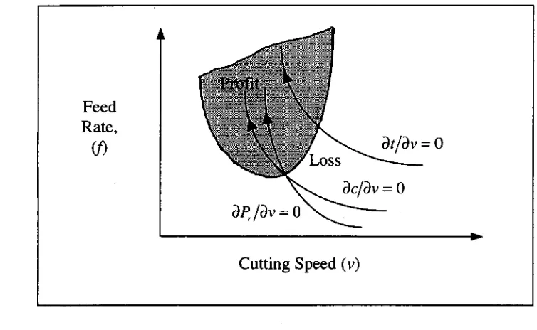
3. The maximum profit rate machining speed ( Vp ) is determined by:

,

(1— n)(kt + k(lc, —nCn(r

n

+ k

m

t

p

)=

where

r =

X = machining constant (for turning) — TcDL 1000s

The maximum profit rate machining speed (vp) can be explicitly expressed from

equation (1.22) for particular values of n. However, if the cutting speed is used as

the only variable then the task becomes more complex and difficult resulting in

the use of numerical methods to find the optimum speed. Using speed as the only

variable and with the aid of computer analysis Wu and Ermer [26] found that the

speed for maximum profit was between the speed for minimum cost (vs) and the

speed (vt) for maximum production. As the unit revenue rn is increased,

approaches vt and deviates from vs and vice-versa. Using the direct analytic

approach, Armarego and Russell [6] considered speed and feed as the variables

based on the maximum profit equation

I —u

P

r t

Chapter 1 - Literature Survey

u

= cost per component

and t = unit production time

The maximum profit speed (v

p

) and maximum profit feed

were derived from

the

aPlav

= 0 and

apdaf =

0 equations. They showed that the high feed-low

speed economic trends were also applicable to the maximum profit. By

comparing ac/3v = 0,

atiav

= 0, and

aPlav

= 0, Armarego and [6] found that

the

aPlav

= 0 and atiav = 0 curves did not intersect the

VI

diagram.

However, the

apdav =

0 curve intersected the

aciav =

0 curve where the profit

rate was zero (Figure 1.7)

Figure 1.7 - Loci of

atiav = o, aciav =

0, and

ap day =

0 curves.

The authors also deduced that the often suggested cutting [7, 51, 52] could incur a

loss between the minimum cost and maximum production rate curves (unless

income was high). Hence, it is suggested that the cutting conditions selected

Hitomi [50] also assumed that it is reasonable from a practical stand-point that the machining speed for the maximum production rate is greater than that for the minimum production cost per piece produced ie

V_C

<

Any value of machining speed between these two optimum values is called the high efficiency speed and is preferable from a managerial stand-point. Hitomi [53, 54] also proved that the maximum profit rate machining speed (vp) exists in

the high efficiency range and found the following relationship

V_c

< Vp <

Chisholm et al [55] found the effect of speed (v) and feed (f) on the cost per component with the aid of numerical and graphical techniques for specific demonstrations. Their observations led to the conclusion that lower minimum unit production costs (u) were obtained when low speed was combined with high feed, as shown in Figure (1.8). Since then other workers [8, 56, 57] have shown similar trends.

Chapter 1 - Literature Survey

Figure 1.8 - Cost per component versus cutting speed for a range of feeds.

1.6.2 Single Pass Turning With Constraints

In single pass turning operations without constraints the most significant economic trend for selecting the optimum cutting conditions is the high feed-low speed. However, when technological constraints are added to this simple case, the optimisation strategies will be different.

1. Optimisation strategies under Machine Tool Feed-Speed Boundary Constraints

Most researchers have pointed out that when selecting optimum cutting

conditions, the highest feed and speed should not exceed the machine tool

maximum tool maximum feed _(fm) and speed (V..) limits [4]. The latter limit

optimised cutting conditions in practice. Armarego and Wong [29] and Wong

[63] presented the initial steps in selecting tool-work combinations and machine

tool by superimposing known values of feeds and speeds of the machine tool with

the

at/av =

the machine feed-speed boundary (feasible area) the machine would be deemed

unsuitable as shown in Figures 1.9 (a) and (b), otherwise Figure 1.9 (c). They

further stated that the high feed-low speed selection was only applicable if

o

feed exponent. By varying the combinations of n and ni Wong [63] was able to

give a feed and speed selection strategy. However, he did not consider the effects

of the machines minimum feed (f,n,n)and minimum speed (17,,in) and the

aof =

effects. As shown in Figure 1.10, five fundamental cases were observed in the V-f

domain. The case where the optimum cutting conditions lie on the machine tool

minimum feed (fm) and minimum speed (V,„,) are shown in Figures 1.10 (a), (b)

and (c). The cases where the optimum machine cutting conditions lie on the

Figure 1.9 - Guide-line for preliminary selection for suitable machine tool [4].

fMAX

fmiN

fMAX

fMIN

fMAX

fMIN

VMIN VMAX

(a)

VmEN VmAx

(c)

VMIN VMAX

(d) •

• denotes optimum cutting condition

VMIN VMAX

(e) Chapter 1 - Literature Survey

1.6.3 Multi-Pass Turning Without Constraints

Single pass turning operations are not always superior to multi pass turning

operations. They are optimum only if the operation is only restricted by the

highest allowable feed, which is not the most general case [3]. When a large

depth of cut is to be removed several passes (multi-pass operations) may have to

be considered. The analysis of multi-pass turning optimisation is much more

complicated than for single-pass turning operations since x speeds and x feeds for

each of the x passes, the number of passes, and x-1 depths of cut have to be

determined.

The question that arises in multi-pass turning operations is which optimisation

strategy to use. Workers such as Chia [15] claimed that the trends and

optimisation strategies used for single-pass operations could be directly applied to

each pass in multi-pass turning operations to establish the constrained optimum

cutting speed and feed, allowing for the diameter variation in each pass. This

approach could provide guide-lines for the optimum d, (depth of cut in ith pass)

distribution and the optimum number of passes x although the numerical search

techniques had to be used.

Kals and Hijink [31] suggested using equal depths of cut in each pass except for

the last pass, while others such as Hinduja et al [66] suggested the use of the

maximum possible depth of cut for all passes except for one. While these

strategies gave the optimum solution for some cases they were not the result of

Chapter 1 - Literature Survey

Unklesbay and Creighton [67] divided the total depth of cut into an appropriately selected integer number. Different combinations of these depth increments were then used to find the optimum depth of cut and the resulting optimum number of passes. Iwata et al [30] showed that the optimum depth of cut and the number of passes only slightly affected the optimum speed and feed. However, they used an equal depth of cut for each pass which Chia [15] claimed to be an unproven strategy.

Lambert and Walvekar [10] and Ermer and ICromodihargjo [11] combined linear programming with geometric programming to optimise multi-pass turning operations and used the Taylor tool-life equation, several practical constraints and minimum cost per component as the economic criteria in their optimisation analysis. The values of depth of cut for each pass were chosen arbitrarily and the optimum speed and feed were determined using geometric and linear programming procedures.

1.6.4 Multi Pass Turning With Constraints

Constrained optimisation analysis and strategies for multi-pass turning operations

with the multiple practical constraints of relevance to rough turning operations

have been shown to be much more complicated than for the corresponding single

pass analysis [4]. This is because the number of passes, the depth of cut, cutting

speed and feed for each pass have to be determined to satisfy the selected

economic criteria whilst not violating any of the constraints in every pass. This

complex case is out the scope of this work. However, the next section is devoted

to an example which demonstrates one of the current strategies used in the

optimisation of constrained multi-pass turning operations.

1.6.4.1 Example of a Strategy Used For The Optimisation of Constrained

Multi-Pass Turning Operations:

The following strategy for the optimisation of constrained multi-pass turning

operations has been developed by Chua M.S., Rahman M., Wong Y.S., and Loh

H.T.[68].

The main objectives of their work were:

"(a) To study the effects of depth of cut, feed rate and cutting speed on the

tool life, cutting forces and power consumption for TiN-coated carbide

tools and Michlin 14 medium carbon steel using design of

Chapter 1 - Literature Survey

(b)

To develop mathematical models to predict tool-life, cutting forces

and power consumption as a function of depth of cut, feed rate and

cutting speed within the operating region; and

(c)

To demonstrate the use of mathematical models in the determination

of optimal cutting conditions using an optimisation technique.

The mathematical modelling of tool-life, cutting forces and power consumption

models for a particular work and tool material involved lots of other factors, such

as ways of holding the workpiece, the geometry of the cutting tool, etc."

However, to facilitate the experimental data collection Chua

[68] only

considered three dominant forces (depth of cut, cutting speed and feed rate) in the

planning of the experiment. They planned the experimental programme using a

complete 3 3 factorial design [69, 70].The range of values of each factor were set at

three levels - low, medium and high as shown in Figure 1.11. This setting gave a

total of 27 experiments to be performed, each having a combination of different

levels of factors as shown in Figure 1.12. The aim of this experiment is to

measure the responses of tool-life, cutting forces and power consumption."

Chua

[68] postulated three mathematical models; the tool-life, cutting force

and power consumption models which in general form are given by

Y= (1)

(1.26)

where Y is the machining response, 4:0 is the response function, and

are the

Y =Cva dY (1.27)

"To facilitate the determination of constants and parameters, these mathematical

models were linearised by performing a logarithm transformation. The

logarithmic transformed mathematical models are given by

lnY=1nC+a lnv-1-13 lnf +y lnd (1.28)

The constants and parameters C, a, Po and y were then solved by using multiple

regression analysis [71]. For the purpose of developing the mathematical model,

both the data for the machining responses and factors were logarithmically

transformed."

The mathematical models developed were used in the formulation of a multi-pass

turning operation problem with the production time as the objective function

subject to process constraints and solved using the sequential quadratic

programming technique [72]. Using this technique the intermediate continuous

solution for multi-pass turning was first determined by assuming that (i) the

cutting conditions for each pass are the same and (ii) the workpiece diameter does

not change during each pass of the cut. For this stage, cutting conditions of, m0=2,

v=178 m/rnin, f=0.25 mm/rev and d=2.00 mm, were used as the feasible starting

point. The optimisation program computed an intermediate optimal solution with

cutting conditions m0=2.58, v=212 m/rnin, f=0.35 mm/rev and d=1.553 mm.

Based on mo, the lower and upper integers, m=2 and m=3, respectively, were

chosen as the number of passes of cut for the integer part of the multi-pass

optimisation. The two-pass and three-passturning optimisation problem for the

Chapter 1 - Literature Survey

intermediate optimal cutting conditions as the starting point. By comparing the

production times, the cutting conditions for the two-pass operation was chosen to

be optimal for turning this particular workpiece, 12.68 minutes as opposed to

14.37 minutes for the three pass operation. Chua

found that the actual

production time for the test was in accordance with the computed production time.

Based on the analysis of variance of each model, Chua

model was independent of the depth of cut as compared with the cutting force and

power consumption models, which were dependent on the depth of cut, the feed

rate and the cutting speed. They also found that the models developed were

approximately 95% representative of this cutting process and the estimated

parameters of each of the models were highly significant at the 99% level of

significance within the operating range.

1.7 Artificial Neural Networks

Neurons are nerve cells and neural networks are networks of such cells eg. the

cerebral cortex of the brain. The notion of imitating the human neural processing

system, cognitive capabilities and biological phenomena to model computation for

artificial intelligence (AI) was introduced about 25 years ago. But it is not until

recently that they are gaining recognition as a viable alternative to performing

complex tasks such as decision making in multi faceted problems. Artificial

neural systems are characterised as a distributed computational system comprising

of a large number of processing units (Figure 1.11) each of which has selected

Output Neurons

Hidden Neurons

Input Neurons

Figure 1.11 - Artificial Neural System.

Biologically each neuron is characterised by a cell body and thin branching

extensions called dendrites and axons (Figure 1.12) which are specialised for

inter-neuron transmission. The dendrites receive inputs from other neurons and

the axon provides output to other neurons. Neurons receive electrochemical input

signals from other neurons to which they are connected at sights on their surface,

called synapses. The input signals are combined in various ways, triggering the

generation of an output signal by the special region near the cell body. However,

the interesting feature of the neurobiological phenomenon is the changing

chemistry of synapse as information flows from one neuron to another. It is this

special feature that researchers in this field of study have tried to emulate.

An idealised model of a neuron is shown in Figure 1.13. The processing elements

are the fundamental building blocks of a neural network. They receive multiple

input connections (which are links between the processing elements and carry

signals between them - each connection may have a weight associated with it for

Magnified Synapse Cell Body

Chapter 1 - Literature Survey

Axon

Figure 1.12 - Neurons and their associated parts.

through the processing element which may fan out to many other processing

elements. The processing element (synapse) consists of a summer and a threshold

detector. The summer adds all the inputs after each of them has been multiplied

with their corresponding weight

0 (1.29)

i=1

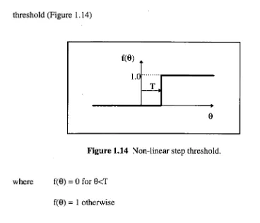
The output f (9 ) is a non-linear function. The simplest non-linear function is a

threshold (Figure 1.14)

Figure 1.14 Non-linear step threshold.

where f(0) =0 for IRT

f(0) = 1 otherwise

However, a more useful non-linear function is the 'soft' threshold (Figure 1.15)

Figure 1.15 - Non-linear 'soft threshold'.

Mathematically this can be described by the sigmoid function which varies

smoothly from 0 to 1 or by the tanh (hyperbolic tangent) function which varies

Chapter 1 - Literature Survey

tanh(x) = 2sigmoid(2x) — 1 (1.30)

The sigmoid can be used in the hidden layer of the NHM network and is given by

1

f (0 - 1 + exp(4 (1.31)

where 0 =147 x + Threshold

The differential of the sigmoid is given by

f - _{[1+ exp(-0 )] 2 — 1+ exp(-0 ) * 1+ exp(-0 )} exp(-0 ) 1 1+ exp(-0 ) —1 (1.32)

or

f = f(0)( 1 - f(0)) (1.33)

In this work one will use the 3-layer feedforward multi layered perceptron using

backpropagation to simulate real time optimisation of machine cutting variables

such as speed and feed using the minimum production time as the economic

criteria. This type of neural network (Figure 1.16) is often called the NHM

network, where N is the input layer, H is the hidden layer and M is the output

Chapter 1 - Literature Survey

•Figure 1.16 - A standard back propagation network comprises 3 layers of

processing elements, fully feed-forward connected.

Mathematically, Figure 1.16 can be represented by Figure 1.17

Input Layer Hidden Layer Output Layer

•th

node jth node kth node

•

0

0

Outputs xi Zj Yk

Indices i, 0...N j, 1...H k, I...M x0=1 weight, weight, uki

wio, threshold of i th node

Chapter 1 - Literature Survey

The basic equations for a multilayered (NHM) network are

Vk

=EU .Z.

1

Z — (1.35)

1+ exp(-0i)

of

=EW

ii

i=0

where yk, represent the linear outputs, Zj is the sigmoid function in the hidden layer only, and Oj represents the weighted sum.

The error is

E = — 24(y — t k)2

2 k=, (1.37)

where tk = true or desired value.

Equation 1.37 is the square root error not the RMS error.

The training task is to vary the weights wji and uki so that the error term (E) is a minimum.

OLD

UkjNEW = U kj + U_kj (1.38)

and

OLD . _a

w.. NEW _{= Wkji W JI} (1.39)

There are many ways of estimating the correction Auk, and Aw,,, but the simplest

and most commonly used is the method of "steepest descent". This method is like

being blindfolded on a hillside and you can move around and from the angle of

your ankles you can tell which way is down and you can take a step in that

direction. You can then test the direction and continue. The length of your step

depends on how steep the hillside is. As it flattens off, your step becomes smaller.

Mathematically this is

aE

Au_{kj =} TI

i ki (1.40)

and

aE

j aW

(1.41)

where = 'step length' or 'learning rate' and is usually about 0.1.

The algorithm one would follow for backpropagation is as follows

(a) Scale all inputs to 0..1 or ±1.

(b) Set all wii and ukj weights to random numbers in the range ±1.

(c) Randomly pick an instance from the training set, ie one set of xi, i = 1..N

and the categories or values required at the outputs.

(d) Feed the values through the net to get the k outputs.

Chapter 1 - Literature Survey

(f) For each wji modify the weight using.

NEW OLD +

" JI "V V kji

aE

where Aw = —1 ,

_aw

and

aE

_{— z (1— z ). x •18 k kj}

aw,,

k =I

(g) For each ukj modify the weight using

u kj

NEW OLD

= ki + CIA _kj

(1.42)

(1.43)

aE

where Au_kj = -11

aukj

aE

and

_au

kj

k

(h) Pick another instance from the training set and repeat from (d) until the net reproduces the training set or does not improve (104 - 108 times is

typical), [74].

Chapter 1 - Literature Survey

t+

W 1 =14,` -FrOw' +aAw1-1 (1.44)

The first two terms in equation 1.44 are as before, the third term is called the

'momentum', a, and it can be as large as 0.9.

Also, the weight correction is proportional to the slope of the error surface ie

aE

LWocyvt-, (1.45)

The slope may go to zero (flat spots) at points that are not at the bottom of holes

(Figure 1.18), for instance at the top or on a shoulder.

Figure 1.18 - Example of flat spots, local and global minimum.

The minimum that is found may not be the 'global' minimum but a 'local'

minimum. There is very little that can be done in this case apart from

exhaustively searching for the global minimum. However, if the local minimum

solves the problem at hand then this case does not matter. If it does matter, then

the search which have to begin again from a different set of random weights with

Chapter 1 - Literature Survey

The momentum term can both speed up the training and help to push through local

minima.

1.8 Concluding Remarks

It is evident from the above survey that many researchers in the field of economics

of machine operations have endeavoured to include practical constraints in their

analysis to develop general trends in cutting operations. While the optimisation

analysis of single-pass turning operations is relatively straightforward, the analysis

of multi-pass turning operations has proven to be a complex task incorporating

many parameters and certain economic criteria, which have to be satisfied

simultaneously.

This thesis is aimed at developing cutting conditions for unconstrained and

constrained single-pass turning operations using machine speed and feed rate as

constraints. The optimisation analysis is based on the maximum production rate

(minimum production time) criterion. Results that are obtained from the classical

mathematical studies are compared to those obtained under the same conditions

on a CNC machine (Mazak Quick Turn 15N) which includes optimisation

hardware/software (Mazatrol T Plus). Finally, the use of a multilayer perceptron

neural networks with back propagation is used as a decision making tool to obtain

Computer Integrated Manufacturing (CIM)

The technology that has had the greatest impact on manufacturing firms over the

last few decades is computer technology applied to production systems [75]. One

area to which this technology is applied is that of computer control. This includes,

computer numerical control (CNC), flexible manufacturing systems (FMS) and

robotics. Other applications of computer systems range from product design to

manufacturing process planning and control. Furthermore, these applications

include the business operations of the company (such as inventory use and

planning, cost accounting, time scheduling, customer billing, etc.). These various

functions constitute the information-processing cycle (because the common

denominator that drives these functions is information in the forms of data and

knowledge) that occurs in a manufacturing firm.

Computer integrated manufacturing uses the computer in the information

processing cycle to integrate the different functions - design, manufacturing and

business operations - into a unified, well-coordinated, and smooth running system.

The two main constituents of CIIvl are computer aided design (CAD) and

I

(EA")

Data Base

roduction planning and Scheduling

Tool & fixture

Design

Chapter 2 - Computer Integrated Manufacturing (CIM)

CAD/CAM systems if the system supports manufacturing as well as design applications.

CAD is a design activity that involves the effective use of the computer to create, modify or document an engineering design with the use of an interactive computer graphics system.

CAM is the effective use of computer technology in the planning, management, and control of the manufacturing function. CAM can be effectively branched out into its separate components as shown in Figure 2.1 below.

Figure 2.1 - CAPP in relation to other computer aided systems.