Active structural acoustic control smart panel with small scale proof mass actuators

ePrints Soton

Copyright © and Moral Rights for this thesis are retained by the author and/or other copyright owners. A copy can be downloaded for personal non-commercial

research or study, without prior permission or charge. This thesis cannot be

reproduced or quoted extensively from without first obtaining permission in writing from the copyright holder/s. The content must not be changed in any way or sold commercially in any format or medium without the formal permission of the

copyright holders.

When referring to this work, full bibliographic details including the author, title, awarding institution and date of the thesis must be given e.g.

AUTHOR (year of submission) "Full thesis title", University of Southampton, name of the University School or Department, PhD Thesis, pagination

UNIVERSITY OF SOUTHAMPTON

FACULTY OF ENGINEERING AND APPLIED SCIENCES

INSTITUTE OF SOUND AND VIBRATION RESEARCH

ACTIVE STRUCTURAL ACOUSTIC CONTROL SMART PANEL WITH SMALL SCALE PROOF MASS ACTUATORS

by

Cristóbal González Díaz

A thesis submitted for the award of Doctor of Philosophy

UNIVERSITY OF SOUTHAMPTON

ABSTRACT

FACULTY OF ENGINEERING AND APPLIED SCIENCE

INSTITUTE OF SOUND AND VIBRATION RESEARCH

Doctor of Philosophy

ACTIVE STRUCTURAL ACOUSTIC CONTROL SMART PANEL WITH SMALL SCALE PROOF MASS ACTUATORS

by Cristóbal González Díaz

This thesis presents a comprehensive study of decentralised feedback control on a smart panel with electrodynamic proof mass actuators and velocity sensors at their footprints. The aim is to provide guidance for the design of light, simple, robust and low cost, control units which can be attached in large numbers to flexible structures in order to control their spatially averaged response and sound radiation at low audio-frequencies.

The first part of the thesis is focused on the identification of simple and effective single channel feedback control laws. In particular the stability properties and control performance produced by Proportional, Integral, Derivative, PI, PD, PID feedback control laws are assessed with reference to two simple problems where a single degrees of freedom system is controlled by an ideal reactive force actuator and by a practical proof mass actuator.

Following this introductory study, the implementation of decentralised feedback control on a smart panel with five control units using proof mass electrodynamic actuators is investigated for the best two cases of Proportional and PID control. In parallel the practical design of small scale control units is explored. In particular the scaling of the stability and control performance properties of a single control unit that implements proportional control is examined using a stability–control formula.

TABLE OF CONTENTS

ABSTRACT... II

TABLE OF CONTENTS...III

LIST OF ILLUSTRATIONS ...VII

LIST OF TABLES ... XVIII

LIST OF TABLES ... XVIII

LIST OF SYMBOLS ... XIX

ACKNOWLEDGEMENTS... XXIII

1 INTRODUCTION...1

1.1 SHORT REVIEW OF ACTIVE CONTROL OF SOUND AND VIBRATION...2

1.2 FEEDBACK VERSUS FEEDFORWARD CONTROL...3

1.3 DECENTRALISED VERSUS CENTRALISED CONTROL...4

1.4 SMART PANELS FOR ACTIVE STRUCTURAL ACOUSTIC CONTROL (ASAC) ...6

1.5 SMART PANELS FOR ACTIVE VIBRATION CONTROL (AVC)...7

1.6 SENSOR-ACTUATOR TRANSDUCER FOR SMART PANELS...8

1.7 SCALING OF TRANSDUCER...9

1.8 SCOPE AND OBJECTIVE...10

1.9 STRUCTURE AND ORGANISATION...11

1.10 CONTRIBUTIONS...12

2 FUNDAMENTAL CONCEPTS OF FEEDBACK CONTROL ...13

2.1 SINGLE DEGREE OF FREEDOM SYSTEM UNDER HARMONIC MOTION OF THE BASE...13

2.2 SDOF SYSTEM UNDER HARMONIC MOTION OF THE BASE WITH A REACTIVE FORCE FEEDBACK CONTROL LOOP...16

2.2.1 Proportional control for implementation of velocity feedback...17

2.2.2 Integral control for implementation of displacement feedback ...18

2.2.3 Derivative control for implementation of acceleration feedback ...18

2.2.4 Proportional-Integral-Derivative (PID) control ...19

2.3.1 Proportional Control: velocity feedback ...22

2.3.2 Integral Control: displacement feedback...23

2.3.3 Derivative Control: Acceleration feedback ...24

2.3.4 PID Control...25

2.4 CONTROL PERFORMANCES. ...27

2.4.1 Proportional Control ...27

2.4.2 Integral Control ...28

2.4.3 Derivative Control ...29

2.4.4 PID Control...30

2.5 SDOF SYSTEM UNDER HARMONIC FORCE WITH A PROOF MASS FORCE ACTUATOR30 2.6 SDOF SYSTEM UNDER HARMONIC FORCE WITH A PROOF MASS FORCE FEEDBACK CONTROL LOOP...34

2.7 STABILITY ANALYSIS...34

2.7.1 Proportional control ...36

2.7.2 Integral control ...37

2.7.3 Derivative Control ...38

2.7.4 PID Control...39

2.7.5 PI Control ...42

2.7.6 PD Control...44

2.8 CONTROL PERFORMANCES...46

2.8.1 Proportional Control ...46

2.8.2 Integral Control ...47

2.8.3 Derivative Control ...47

2.8.4 PID Control...48

2.8.5 PI control ...48

2.8.6 PD Control...49

2.9 SUMMARY...50

3 MODELLING AND STUDY OF SMART PANELS WITH DECENTRALISED FEEDBACK CONTROL USING PROOF MASS ELECTRODYNAMIC ACTUATORS...52

3.1 MODEL PROBLEM...53

3.2 STABILITY ANALYSIS...60

3.2.1 Stability of a single control unit...62

3.2.2 Stability of five decentralised control units...77

3.3.1 Control performance produced by single control unit...83

3.3.2 Control performance produced by five decentralised control units ...88

3.4 SUMMARY...90

4 STABILITY AND CONTROL PERFORMANCE SCALING STUDY...92

4.1 ACTUATION MECHANISM...92

4.2 STABILITY OF A DIRECT VELOCITY FEEDBACK LOOP...97

4.3 CONTROL PERFORMANCES...99

4.4 ELECTRODYNAMIC ACTUATION FORCE SCALING LAWS...102

4.5 SCALING LAWS OF THE MECHANICAL COMPONENTS OF THE ACTUATOR...103

4.6 SCALING LAWS OF THE DYNAMIC CHARACTERISTIC OF THE PROOF MASS ACTUATOR ...104

4.7 SCALING LAWS FOR THE STABILITY AND PERFORMANCE PARAMETERS...105

4.8 SUMMARY...108

5 DESIGN AND TEST OF A PROTOTYPE DVFB CONTROL UNIT WITH A SMALL SCALE PROOF MASS ACTUATOR ...109

5.1 DESIGN OF THE PROTOTYPE PROOF MASS ACTUATOR...109

5.2 OPEN LOOP STABILITY ANALYSIS...113

5.3 CLOSED LOOP CONTROL PERFORMANCE ANALYSIS...115

5.4 SUMMARY...116

6 IMPLEMENTATION OF DECENTRALISED CONTROL ...117

6.1 STABILITY AND CONTROL PERFORMANCE THEORETICAL ANALYSIS...118

6.1.1 Plate–actuators coupled model...118

6.1.2 Passive effects of the actuators ...125

6.1.3 Stability of the five channel feedback control system...126

6.1.4 Control performances ...128

6.2 PROTOTYPE SMART PANEL WITH FIVE DECENTRALISED CONTROL UNITS...130

6.3 STABILITY-CONTROL PERFORMANCE TESTS...132

6.3.1 Stability analysis ...132

6.3.2 Control performance...133

6.4 GLOBAL CONTROL EFFECT PRODUCED BY THE SMART PANEL...135

6.4.1 Kinetic energy of the panel measured with laser vibrometer ...136

6.4.2 Total sound power radiated measured in anechoic room...142

7 CONCLUSION...149

FUTURE WORK ...152

APPENDIX A ...153

LIST OF ILLUSTRATIONS

Figure 1.1: Illustration from active control patent given to Paul Lueg in 1936....2

Figure 1.2: Scheme of a Feed-forward control system....3

Figure 1.3: Scheme of a feedback control system....4

Figure 1.4: Active Structural Acoustic Control (ASAC) with a large number of

centralised sensor-actuators pairs....6

Figure 1.5: Active Structural Acoustic Control (ASAC) with a large number of

decentralised collocated sensor-actuators pairs....7

Figure 2.1: Single degree of freedom system under harmonic motion of the base....13

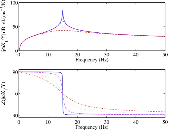
Figure 2.2: Modulus and phase of the ratio between the velocity of the proof mass and the displacement of the base of the system shown in Figure 2.1(a) when the

system is damped by ξ1=0.001 (solid line), ξ2=0.1 (dashed line), ξ3=0.4 (dotted

line) or ξ4=0.8 (dash-dot line)....15

Figure 2.3: SDOF under harmonic motion in the base with feedback control....16

Figure 2.4: Block diagram of feedback control system implemented on the SDOF

system....20

Figure 2.5: Frequency response functions; amplitude (top left), phase (bottom left) and Nyquist plot (right) of the open loop sensor–actuator frequency response function in the frequency range between 0-50 Hz when a Proportional control

is used....22

Figure 2.6: Frequency response functions; amplitude (top left), phase (bottom left) and Nyquist plot (right) of the open loop sensor–actuator frequency response function in the frequency range between 0-50 Hz when an Integral control is

used....23

function in the frequency range between 0-50 Hz when a Derivative control is

used....24

Figure 2.8: Frequency response functions; amplitude (top left), phase (bottom left) and Nyquist plot (right) of the open loop sensor–actuator frequency response

function in the frequency range between 0-50 Hz when a PID control is used....26

Figure 2.9: Zoom of the Nyquist plot shows in Figure 2.8....26

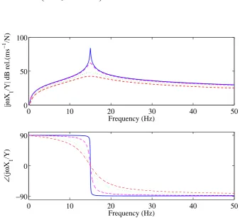
Figure 2.10: Modulus and phase of the ratio between the velocity of the proof mass and displacement of the base of the system shown in Figure 2.3(a) when the

system has a small damping ratio (ξ=0.001) and different values of gain;

g1=0; no-gain (solid line), g2=0.1 (dashed line), g3=0.5 (dotted line) or g4=1

(dash-dot line) when a Proportional control is used....27

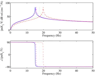
Figure 2.11: Modulus and phase of the ratio between the velocity of the proof mass and the displacement of the base of the system shown in Figure 2.3(a) when the

system has a small damping ratio (ξ=0.001) and different values of gain;

g1=0; no-gain (solid line), g2=10 (dashed line), g3=50 (dotted line) or g4=100

(dash-dot line) when an Integral control is used....28

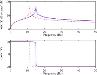
Figure 2.12: Modulus and phase of the ratio between the velocity of the proof mass and the displacement of the base of the system shown in Figure 2.3(a) when the

system has a small damping ratio (ξ=0.001) and different values of gain;

g1=0; no-gain (solid line), g2=0.001 (dashed line), g3=0.005 (dotted line) or

g4=0.01 (dash-dot line) when a Derivative control is used....29

Figure 2.13: Modulus and phase of the ratio between the velocity of the proof mass and the displacement of the base of the system shown in Figure 2.3(a) when the

system has a small damping ratio (ξ=0.001) and different values of gain;

gk1=0, gc1=0, gm1=0; no-gain (solid line), gk2=10, gc2=0.1, gm2=0.001; (dashed

line), gk3=50, gc3=0.5, gm3=0.005 (dotted line) or gk4=100, gc4=1, gm4=0.01

(dash-dot line) when a PID control is used....30

Figure 2.14: DOF system under harmonic force when Fc=0....31

Figure 2.15: Modulus and phase of the velocities per unit force F1 of the system to be

system shown in Figure 2.14(a) when there is no active vibration control

considering different values of damping ratio; ξ1,1=0.0001 and ξ2,1=0.001

(solid line), ξ1,2=0.005 and ξ2,2=0.05 (dashed line), ξ1,3=0.01 and ξ2,3=0.1

(dotted line), ξ1,4=0.03 and ξ2,4=0.3 (dash-dot line) or ξ1,5=0.08 and ξ2,5=0.8

(dotted line)....33

Figure 2.16: Two DOF under harmonic force with feedback....34

Figure 2.17: Block diagram of Feedback Control implemented on the Two DOF

system....35

Figure 2.18: Frequency response functions; amplitude (top left), phase (bottom left) and Nyquist plot (right) of the open loop sensor–actuator frequency response function in the frequency range between 0-100 Hz when a Proportional control

is used....36

Figure 2.19: Frequency response functions; amplitude (top left), phase (bottom left) and Nyquist plot (right) of the open loop sensor–actuator frequency response function in the frequency range between 0-50 Hz when an Integral control is

used....37

Figure 2.20: Frequency response functions; amplitude (top left), phase (bottom left) and Nyquist plot (right) of the open loop sensor–actuator frequency response function in the frequency range between 0-100 Hz when a Derivative control is

used....38

Figure 2.21: Control function when a PID Control is used....40

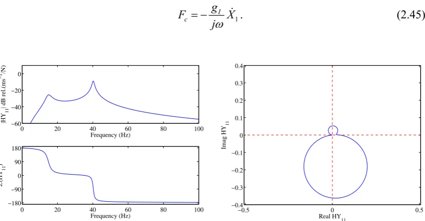
Figure 2.22: Frequency response functions; amplitude (top left) and phase (bottom left). Nyquist plot (right plot) for the frequency response functions between a

collocated ideal velocity sensor in the mass to be controlled (m1) and force

actuator in the 0-100 Hz frequency range in a two DOF when a PID Control is

used....40

Figure 2.23: Zoom of the Nyquist plot shown in Figure 2.22....41

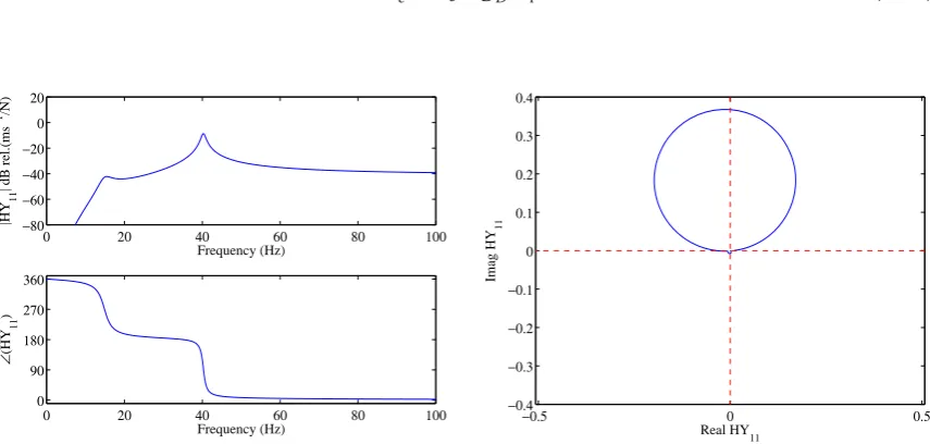
Figure 2.25: Frequency response functions; amplitude (top left) and phase (bottom left). Nyquist plot (right plot) for the frequency response functions between a collocated ideal velocity sensor in the mass to be controlled and force actuator

in the 0-100 Hz frequency range in a two DOF when a PI Control is used....43

Figure 2.26: Zoom of the Nyquist plot shown in Figure 2.26....43

Figure 2.27: Control function when a PD Control is used....44

Figure 2.28: Frequency response functions; amplitude (top left) and phase (bottom left). Nyquist plot (right plot) for the frequency response functions between a collocated ideal velocity sensor in the mass to be controlled and force actuator

in the 0-100 Hz frequency range in a two DOF when a PD Control is used....45

Figure 2.29: Zoom of the Nyquist plot shown in Figure 2.28....45

Figure 2.30: Modulus of the ratio between velocity of the mass of the system to be controlled and the harmonic force of the system shown in Figure 2.16(a) when

a Proportional Control is used and different values of gain; g1=0; no-gain

(solid line), g2=10 (dashed line), g3=50 (dotted line) or g4=100 (dash-dot line)....46

Figure 2.31: Modulus of the ratio between velocity of the mass of the system to be controlled and harmonic force of the system shown in Figure 2.16(a) when a

Integral Control is use and different values of gain; g1=0; no-gain (solid line),

g2=10 (dashed line), g3=20 (dotted line) or g4=60 (dash-dot line)....47

Figure 2.32: Modulus of the ratio between velocity of the system to be controlled and harmonic force of the system shown in Figure 2.16(a) when a Derivative

Control is use and different values of gain; g1=0; no-gain (solid line), g2=10

(dashed line), g3=20 (dotted line) or g4=60 (dash-dot line)....47

Figure 2.33: Modulus of the ratio between velocity of the system to be controlled and the harmonic force of the system shown in Figure 2.16(a) when a PID Control

is use and different values of gain; g1=0; no-gain (solid line), g2=10 (dashed

line), g3=20 (dotted line) or g4=60 (dash-dot line)....48

and different values of gain; g1=0; no-gain (solid line), g2=10 (dashed line),

g3=20 (dotted line) or g4=60 (dash-dot line)....49

Figure 2.35: Modulus of the ratio between velocity of the system to be controlled and harmonic force of the system shown in Figure 2.16(a) when a PD Control is

use and different values of gain; g1=0; no-gain (solid line), g2=10 (dashed

line), g3=20 (dotted line) or g4=60 (dash-dot line)....49

Figure 3.1: Schematic view of the smart panel with five control units made of a proof-mass electro-dynamic actuator with an ideal velocity error sensor at its

base....53

Figure 3.2: Block diagram of a multichanel feedback control system implemented on

the plate....60

Figure 3.3: Force transmitted to the base structure per unit driving current (a) or voltage (b) by an electro-dynamic actuator when the dynamic effect of the base

and coil masses, mb, are (solid lines) or are not (faint lines) taken into account....62

Figure 3.4: Proportional control function....64

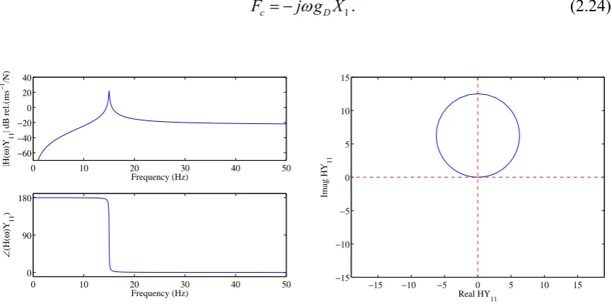
Figure 3.5: Bode (a, b) and Nyquist plots (c, d) of the open loop sensor–actuator FRF when a Proportional feedback loop is implemented for current-driven (a, c) and voltage-driven (b, d) control actuators when the dynamic effect of the

base and coil masses, mb, are (solid lines) or are not (faint lines) taken into

account (a, b)....65

Figure 3.6: Integral control function....66

Figure 3.7: Bode (a, b) and Nyquist plots (c, d) of the open loop sensor–actuator FRF when an Integral feedback loop is implemented for current-driven (a, c)

and voltage-driven (b, d) control actuators....67

Figure 3.8: Derivative control Function....69

Figure 3.9: Bode (a, b) and Nyquist plots (c, d) of the open loop sensor–actuator FRF when a Derivative feedback loop is implemented for current-driven (a, c)

Figure 3.10: PID control function....71

Figure 3.11: Bode (a, b) and Nyquist plots (c, d) of the open loop sensor–actuator FRF when a PID feedback loop is implemented for current-driven (a, c) and

voltage-driven (b, d) control actuators....72

Figure 3.12: PI control function....73

Figure 3.13: Bode (a, b) and Nyquist plots (c, d) of the open loop sensor–actuator FRF when a PI feedback loop is implemented for current-driven (a, c) and

voltage-driven (b, d) control actuators....74

Figure 3.14: PD control function....75

Figure 3.15: Bode (a, b) and Nyquist plots (c, d) of the open loop sensor–actuator FRF when a PD feedback loop is implemented for current-driven (a, c) and

voltage-driven (b, d) control actuators....76

Figure 3.16: Loci of det[I+GccH]=0 when five Proportional Control loops are

implemented by current-driven (a) and voltage-driven (b) control actuators....79

Figure 3.17: Loci of the eigenvalues of the matrix Gcc (jω)H(jω). Current-driven

actuators....79

Figure 3.18: Loci of the eigenvalues of the matrix Gcc (jω)H(jω). Voltage-driven

actuators....80

Figure 3.19: Loci of det[I+GccH]=0 when five PID Control loops are implemented

by current-driven (a) and voltage-driven (b) control actuators....80

Figure 3.20: Loci of the eigenvalues of the matrix Gcc(jω)H(jω). Current-driven

actuators....81

Figure 3.21: Loci of the eigenvalues of the matrix Gcc(jω)H(jω). Voltage-driven

actuators....81

functions are implemented with a set or rising control gains up to that which produces the best frequency averaged reduction of vibration with a stable

feedback loops....84

Figure 3.23: Total flexural kinetic energy of the plate when the control actuator number 1, as shown in Figure 3.1, is current- or voltage-driven (respectively left- and right-hand side plots) and PID, PI and PD control functions are implemented with a set or rising control gains up to that which produces the

best frequency averaged reduction of vibration with a stable feedback loops....87

Figure 3.24: Normalized frequency averaged total kinetic energy in the range between 5 Hz and 1 kHz as a function of the control gain produced by the control unit number 1, as shown in Figure 3.1, when the actuator is driven by current (a) or voltage (b). Solid lines: proportional control; dashed lines: integral control; dotted lines: derivative control; faint line: PI control; faint dash-dotted lines: PD control dash-dotted lines: PID control, these two last

lines are overlapped by the PID and Proportional lines respectively....88

Figure 3.25: Total flexural kinetic energy of the plate when the five control actuators shown in figure 1 are current- or voltage-driven (respectively left- and right-hand side plots) and Proportional and PD control functions are implemented with a set or rising control gains up to that which produces the best frequency

averaged reduction of vibration with five stable feedback loops....89

Figure 3.26: Normalized frequency averaged total kinetic energy in the range between 5 Hz and 1 kHz as a function of the control gains when the five

actuators shown in Figure 3.1 are current- (a) or voltage-driven (b). Solid

lines: proportional control; dash-dotted lines: PID control....90

Figure 4.1: Proof mass electrodynamic force actuator: a) sketch b)

electro-mechanical schematic....94

Figure 4.2: Force transmitted to the base structure per unit driving current. Thick

line heavily damped actuator (Ca=3.3 N/ms-1), dotted line lightly damped

actuator (Ca=0.5 N/ms-1)....96

Figure 4.4: Bode (a) and Nyquist (b) plots of the open loop sensor-actuator FRF

gGcc(ω), assuming g=1 when a proportional feedback loop is used for current

control....98

Figure 4.5: Amplitude of the response at the control position per unit primary force when there is no control (thick line), and when the feedback control loop implements a)moderate control gain (dotted line) and b) the maximum control

gain that guarantees stability (dashed line)....101

Figure 5.1: Photo of the small scale electrodynamic proof mass actuator....110

Figure 5.2: Internal stress for a 316N/m suspension stiffness as function of spring

radius....112

Figure 5.3: Simulated (a) and measured (b) Bode plots of the open loop frequency response function between the error sensor signal and the input signal to the analogue control system when sole the control unit N.2 is mounted on the plate

considered in the Figure 3.1....113

Figure 5.4: Simulated (a) and measured (b) Bode plots loop frequency response function between the error sensor signal and the input signal to the analogue control system when sole the control unit N.2 is mounted on the plate

considered Figure 3.1....114

Figure 5.5: Simulated (a) measured (b) velocity at the error sensor N.2 per unit primary force without actuator (faint line), with actuator and no control (thick line) and with actuator when a moderate feedback control gain is implemented

(dotted line) and very high control gain (dashed line)....115

Figure 6.1: Smart panel with five decentralised velocity feedback control units using proof mass electrodynamic actuators. The panel is excited by a shaker acting

on the top left corner of the panel. Dimensions are in mm....118

Figure 6.2: Schematic with the notation for the velocity and force functions used in

the mobility impedance model....119

Figure 6.3: Block diagram of the multichanel feedback control system implemented

Figure 6.4: Kinetic energy per unit primary force of the panel with no control units (faint line) and with five control units (thick line). (a) theoretical prediction;

(b) experimental measurement with a scanning laser vibrometer....125

Figure 6.5: Loci of the eigenvalues of the 5x5 matrix of sensor-actuator FRFs GcaH

simulated between 5 Hz and 50 KHz....127

Figure 6.6: Simulated Kinetic energy per unit primary force of the panel with no control units (faint line), with five control units when the feedback loops are left open (thick line) and when the five feedback loops are closed with the

maximum control gain that guarantees stability (dotted line)....129

Figure 6.7: Photograph of the box test rig and smart panel with five proof mass

actuators for the implementation of decentralised velocity feedback loops....130

Figure 6.8: Photograph of the complete experimental setup with the box test rig and

the control equipment: signal conditioner and controller (left)....131

Figure 6.9: Loci of the eigenvalues of the 5x5 matrix of sensor–actuator FRFs

measured between 5 Hz and 28 KHz....133

Figure 6.10: Measured velocities at the five error sensors per unit force excitation to the plate with no actuators (faint lines), with actuators and no control (thick lines) and with actuators and implementing the maximum control gains that

guarantee stability (dotted lines)....134

Figure 6.11: Measured narrow band spectra of kinetic energy of the panel derived from the spatially averaged response of the panel measured with a scanning laser vibrometer when the panel is excited by the shaker (a) and by the loudspeaker in the cavity (b). Faint line: response of the panel with no control units; thick line: response of the panel with the five control units; dotted line: response of the panel with the five control units implementing decentralised

velocity feedback control....137

control units; red (centre) bar: response of the panel with the five control units; green (right) bar: response of the panel with the five control units

implementing decentralised velocity feedback control....139

Figure 6.13: Response of the smart panel excited by the shaker at (a) 82.97 Hz resonance frequency, which is controlled by the (1,1) mode of the panel, and (b) at the 123.4 Hz resonance frequency, which is controlled by the (2,1) mode of the panel. Top plots response of the panels with no control actuators. Centre plots, response of the panels with the five control units. Bottom plots, response of the panels when the five units implement decentralised velocity feedback

control loops....140

Figure 6.14: Response of the smart panel excited by the loudspeaker at the (a) 84.4 Hz resonance frequency, which is controlled by the (1,1) mode of the panel, and (b) at the 128.9 Hz resonance frequency, which is controlled by the (2,1) mode of the panel. Top plots response of the panels with no control actuators. Centre plots, response of the panels with the five control units. Bottom plots, response of the panels when the five units implement decentralised velocity

feedback control loops....141

Figure 6.15: Measured narrow band spectra of the total sound power radiated (0-1kHz) derived from the measured sound pressure in nine positions around the box in an anechoic room when the panel is excited by the shaker (a) and the loudspeaker in the cavity (b), white noise. Faint (blue) line: response of the panel with no control units; thick (red) line: response of the panel with the five control units; dotted (green) line: response of the panel with the five control

units implementing decentralised velocity feedback control....143

Figure 6.16: Measured narrow band spectra of the total sound power radiated (0-5kHz) derived from the measured sound pressure in nine positions around the box in an anechoic room when the panel is excited by the shaker (a) and the loudspeaker in the cavity (b), white noise. Faint (blue) line: response of the panel with no control units; thick (red) line: response of the panel with the five control units; dotted (green) line: response of the panel with the five control

Figure 6.17: Measured third octave band spectra total sound power radiated between 0 and 1kHz derived from the measured sound pressure in nine positions around the box in an anechoic room when the panel is excited by the shaker (a) and the loudspeaker in the cavity (b), white noise. Blue (left) bar: sound radiated by the panel with no control units; red (centre) bar: sound radiated by the panel with the five control units; green (right) bar: sound radiated by the panel with the five control units implementing decentralised

velocity feedback control....145

Figure 6.18: Measured third octave band spectra total sound power radiated between 0 and 5kHz derived from the measured sound pressure in nine positions around the box in an anechoic room when the panel is excited by the shaker (a) and the loudspeaker in the cavity (b), white nose. Blue (left) bar: sound radiated by the panel with no control units; red (centre) bar: sound radiated by the panel with the five control units; green (right) bar: sound radiated by the panel with the five control units implementing decentralised

velocity feedback control....146

Figure A.1 Modulus of the twenty five open loop frequency response functions between the five sensors and five actuators of the decentralised control

systems....153

Figure A.2: Phase of the twenty five open loop frequency response functions between

LIST OF TABLES

Table 2.1: Physical parameters for the elements in the SDOF system....15

Table 2.2: Physical parameters for the Proportional, Integral and Derivative Control constants....25

Table 2.3: Physical parameters for the elements in the SDOF system....33

Table 2.4: Physical parameters for the Proportional, Integral and Derivative Control constants used in the two DOF system....40

Table 3.1: Geometry and physical parameters for the panel....54

Table 3.2: Physical parameters for the actuators....54

Table 4.1: Geometry and physical parameters for the panel....93

Table 4.2: Geometry and Physical parameters for the actuators....93

LIST OF SYMBOLS

Abbreviations

j imaginary unit (= −1)

N number of considered mode shapes

n index of mode shape

I identity matrix

μ0 4π10-7Hm-1

π ~3.1415926535, ratio of circumference to diameter of a circle

g 9.81ms-2_{, gravity constant}

Parameters

ω0,i fundamental resonance of the inertial actuators [rad s-1]

fn,i natural frequency of the actuators [Hz]

ω circular frequency [rad s-1]

ωn nth natural frequency of the plate [rad s-1]

φn(x,y) nth mode shape of the plate evaluated at position x, y [-]

φ(x,y) row vector with the amplitudes of the modes at position x, y [-]

ρs mass density of the plate [kg m-3]

Λ modal normalization factor [kg]

ηs loss factor of the plate [-]

lx plate length [m]

ly plate width [m]

hs plate thickness [m]

xp x coordinate of primary force position [m]

yp y coordinate of primary force position [m]

xc1 x coordinate of control system 1 [m]

yc1 y coordinate of control system 1 [m]

xc2 x coordinate of control system 2 [m]

yc2 y coordinate of control system 2 [m]

xc3 x coordinate of control system 3 [m]

yc3 y coordinate of control system 3 [m]

xc4 x coordinate of control system 4 [m]

xc5 x coordinate of control system 5 [m]

yc5 y coordinate of control system 5 [m]

Es Young’s modulus of plate material [N m-2]

νs Poisson’s ratio [-]

mi actuators moving mass [kg]

mb,i actuators housing mass [kg]

ψi actuators electrodynamic transducer coefficient of the coil [N A-1]

ki actuators suspension stiffness coefficient [N m-1]

ci actuators viscous damping coefficient [N s m-1]

Re,i actuators electrical resistance of the driving coil [Ω]

Le,i actuators electrical self-inductance of the driving coil [H]

kP proportional control constant [-]

kI integral control constant [-]

kD derivative control constant [-]

g feedback gain [various]

gI,max max control gain for the current-driven [various]

gU,max max control gain for the voltage-driven [various] H diagonal matrix with the feedback control function [various]

Ψi transducer coefficient of the coil [N A-1]

Ψ diagonal matrix with the transducer coefficients Ψi [N A-1… N A-1]

T total kinetic energy [J]

d actuator stroke [m]

Bgo magnetic flux density at the outer diameter of the air gap [Wb m-2]

Bgi magnetic flux density at the inner diameter of the air gap [Wb m-2]

Bw magnetic flux density in the outer wall of the yoke [Wb m-2]

Bm magnetic flux density in the permanent magnet [Wb m-2]

Ai diameter of the hole in the permanent magnet [m]

Ad diameter of the permanent magnet [m]

b height of the permanent magnet [m]

s air gap width [m]

hg air gap height [m]

hgl height of the lower yoke [m]

Br remanence of the permanent magnet [Wb m-2]

Hl coercivity of the permanent magnet [A m-1]

p configuration factor of magnetic circuit [-]

ρwi electric resistivity of coil wire [V / (Am)]

P electrical power dissipated in electrodynamic actuator [W]

Bg magnetic flux density in the air gap [Wb m-2]

Phasors

fp primary excitation force [N]

fai secondary excitation force [N]

fa secondary excitation force vector with fa1… fa5 [N…N]

w _cr transverse velocity at the error control position [m s-1]

w_c transverse velocity vector with w_c1…w_c5 [m s-1…m s-1]

w _{m i,} transverse velocity of the proof-mass [m s-1]

w_m vector with the transverse proof-mass velocities w_m1…w_m5 [m s-1…m s-1]

fmi force between the proof-mass and the suspension spring [N] fm vector with the forces between the proof-masses and the suspensions springs

[N…N]

w column vector with components w_c and w_m [m s-1…m s-1]

f column vector with components faand fm [N…N]

fc,i reactive forces generated by the linear electro-dynamic motor [N]

fc column vector with the reactive forces fc1… fc5 [N…N]

Ic,i electrical current in the coil of the ith actuators [A]

Ic column vector with five currents in the coils [A…A]

Us,i electrical driving voltage [V]

Uc column vector with the five driving voltage [V…V]

Impedances and mobilities

Ycp,r transfer mobility of the plate between primary and secondary

Actuators [m s-1 / N]

Ycc,r point mobility of the plate at the position of the secondary actuators [m s-1 / N] Ycp matrix with the transfer mobility of the plate between primary and secondary

Actuators [m s-1 / N]

Ym,ii mobility of the proof-mass [m s-1 / N]

Ym matrix with the mobilities of the proof-mass [m s-1/N…ms-1/N] Yc diagonal matrix with components Yccand Ym [m s-1 / N … m s-1 / N] Yp column vector with components Ycpand 0 [m s-1 / N … m s-1 / N] V column vector with components I5x5 and –I5x5

Zs,ii impedance of the spring-damper [N s m-1]

Zs diagonal matrix with the impedances of the springs-damper [N s m-1]

ZAct,ii impedance of the base mass [N s m-1] ZAct diagonal matrix with the impedance of the base mass [N s m-1]

Z square matrix with impedance components [N s m-1]

ACKNOWLEDGEMENTS

First and foremost, I am in deep gratitude for the guidance and support of my supervisor, Prof. Paolo Gardonio for his invaluable guidance towards the completion of this thesis. I have benefited immensely not only from his unique knowledge and deep understanding of the subject matter of this thesis but equally from the truly generous and sincere manner in which he has always approached my aspirations or concerns.

Also, I wish to express my sincere thanks to Prof. Steve Elliott for giving me the opportunity to work at Signal Processing and Control Group.

I also extend a heartfelt thanks to Yohko, Christoph and Olie who worked hand-in-hand with me in the laboratory and helped me maintain some form of sanity throughout endless experimental problems. Without their help, I would still be trying to figure out the dynamic analysis portion of this research.

Friendships formed at the ISVR and University of Southampton have also helped keep me grounded during some of the most trying times of my academic work. I extend my thanks to Matt, Andrianakis, Paulo, Beda, Timos, Miguelito, Samy, Tasoulita, Battaner, Simon, Mirko, Eduardo, Emery, Emiliano, Norma, Disha, Pierrick, Lars, Giovanni, Neven, Jens, Antoine, Bene, Claudio, Carolina, Manu, Manuel, Maria, Viky, Maria Carmen, and everyone else who has ever been there for me.

During my study at ISVR there is probably not a single member of staff, technician or student that I have not turned to at one time or another for help or advice and I would like to thank them all. I would particularly like to thank Antony Wood, Rob Stansbridge, Tony Edgeley and Nigel Davies for the time and effort they have spent on my various experimental projects and Maureen Strickland for all the solutions she has provided.

También es necesario dar las gracias a las cinco más importantes personas de este mundo, mis padres y hermanos. Sin su amor y su apoyo financiero durante mis estudios, no habría tenido la oportunidad de continuar mi educación. Gracias a Prisci, Pilar, Mariano, Olga y Pili, y mi familia entera.

Quería agradecer a mi familia adoptiva parisina todo su apoyo, sin ellos no habría sido posible haber llegado tan lejos como he llegado. Gracias a Jesús, Manu Blasco, Octavio, Sara y todos los amigos que allí conocí… incluso a aquellos que casi arruinan mi carrera profesional… gracias David Putero, Alberto Putero, Manu Climent, Fernando y todos los demás.

1 INTRODUCTION

In many engineering systems it is important to control air-borne and structure-borne sound radiation by partitions in order to prevent discomfort. In particular, vibration of panels and shell structures may generate high levels of interior noise in transportation vehicles such as aircrafts, helicopters, cars, trains, etc [1-3]. The background of this study is the control of vibration of thin panels in order to avoid excessive vibration and sound radiation levels. Vibration and sound radiation control can be achieved with passive means such as mass, damping and stiffness treatments applied on the radiating structure [4,5]. In general, these methods have been proved to be efficient in the high audio frequency range. However, they are quite bulky and tend to be less effective in the low audio frequency range [6], where the mechanical responses of structures are characterised by well–separated resonances [7,8]. In order to control low frequency vibration and sound radiation, active control methods have been considered [7,9,10].

‘Smart panels’ are adaptive structures with sensor and actuator transducers directed by a controller capable of modifying response of the structure in presence of time-varying environmental and operational conditions [11].

analysed using scaling laws applied to a ‘stability-performance’ formula specifically derived for this study.

1.1 Short review of Active control of sound and vibration

Frequently both passive and active systems are used together to reduce vibration and sound radiation. Active control essentially tries to eliminate sound or vibration components by adding the exact opposite sound or vibration. The phase describes the relative position of the wave in its rising and falling cycle. If two waves are in phase, they rise and fall together, whilst if they are exactly out of phase, one is rises as the other falls, and so they cancel out. An active control system can alter the amplitude of the control waves to ensure that the primary wave is cancelled. This is usually achieved by monitoring the result of both waves together and adapting the controlled waveform to reduce the total amplitude until cancellation is achieved. The waveforms may represent the acoustic pressure variations in a duct or enclosure, or the displacement of a vibrating structure. The principle of active control of sound and vibration is not new. It was first introduced by Lueg (1936) [12] in a patent as is shown in the Figure 1.1.

Figure 1.1: Illustration from active control patent given to Paul Lueg in 1936.

However it took about two decades before the first single-channel analogue control system was built [13,14]. The wider application of active control and the development of systems with many microphones and many loudspeakers have been made possible by the development of integrated circuits, which implement Digital Signal Processing (DSP) algorithms, such as those used in active control [15-17].

1.2 Feedback versus Feedforward control

Feed-forward control systems require a reference signal well correlated to the disturbance to be controlled. Thus they normally provide good control effects for tonal disturbances that can be easily characterised far in advance [15,18].

r(ω )

s(ω )

Primary source with reference sensor

- (

H ω

)

Figure 1.2: Scheme of a Feed-forward control system.

As schematically shown in the Figure 1.2, the reference signal, r(ωo), is detected by the primary source and used to obtain the signal s(ωo) that drives the control actuator.

For random, wide-band disturbances, feedback control schemes should be utilized. The implementation of feedback control system does not require a reference signal. These systems can provide good control performance regardless of the type of disturbance to be controlled, provided the sensor and actuator transducers are collocated and dual [11,19]. Collocation is a geometrical characteristic where point sensors and actuators are placed in the same position on the structure. Duality is a physical property where the actuator and sensor excite and detect the vibrations of a structure in the same manner.

p(ω)

Primary source - (H ω) error sensor

electrical controler

Figure 1.3: Scheme of a feedback control system.

The construction of distributed pairs of collocated and dual sensor-actuator transducer is not an easy task. One of the most common ways is by using the same type of transducers and by locating the two transducers in the same position.

1.3 Decentralised versus Centralised control

Feedback control systems for vibro-acoustic control can be classified in three categories: a) Multiple Input Multiple Output (MIMO) systems with fully coupled arrays of error

sensor and actuators,

b) Decentralised MIMO control schemes with arrays of independent sensor–actuator pairs, and

c) Single Input Single Output (SISO) active control schemes, using distributed sensor–actuator pairs [7].

Fully coupled MIMO systems are difficult to implement in practice, since a reliable model of the response functions between all sensors and actuators is required by the controller [11,19]. Moreover they require a lot of cabling to connect all sensors and actuators to the controller. As a result the system tends to be heavy, costly and requires a lot of maintenance. Finally centralised controllers are not robust systems since they would not work properly if one sensor or actuator fails.

control is implemented. Therefore, the main issue of decentralised MIMO control is concerned with the design of collocated and dual sensor–actuator pairs [7]. When decentralised velocity feedback loops are implemented in such a way as to generate active damping, both the frequency average vibration and sound radiation of the structure are reduced, provided an optimal gain is implemented such that the damping action is maximised without pinning the structure at the control positions [27]. The optimally tuned active dampers reduce the amplitudes of the well separated low frequency resonances of the structure and thus the frequency averaged vibration and sound radiation at low frequencies. Previous work [28] has shown that, to produce the best performances, there is no need of fine tuning of the control gains. Also, when large arrays of control units are used, there is no need to specially position the control systems. The desired active damping effect will be generated provided the units are evenly spread over the whole surface of the structure to be controlled. These properties make decentralised control a very appealing and robust approach where the focus is just on the design of simple and effective feedback control units using closely located sensor–actuator pairs.

In principle, SISO feedback control systems using distributed sensor–actuator pairs specifically designed to minimize the most efficient radiation modes of the radiating structure [29] form the simplest and most convenient solution for active structural acoustic control. However, they normally require strain transducers, such as piezoelectric transducers, which cannot be easily used to form matched and collocated sensors and actuator pairs that guarantee unconditionally stable feedback control loops [30].

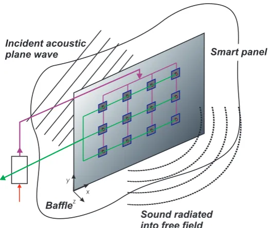
1.4 Smart panels for Active Structural Acoustic Control (ASAC)

As schematically shown Figure 1.4 in Active Structural Acoustic Control (ASAC) trough partitions, structural sensors and actuators are closely attached or even integrated into the walls in order to modify or control the vibration of the partitions and reduce the sound transmission [31]. Most of this research was motivated by the reduction of air-borne or structure-borne noise transmission of the fuselage walls or marine hulls in aerospace and naval applications [1-3,32,33]. The first ASAC systems were built using adaptive feed-forward control. In this case a set of error sensors was required for the detection of the total sound power radiated to be minimised. Thus, although the actuators were integrated into the walls, the error signal was taken from the acoustic measurements in the space under acoustic control. ASAC systems tend to be most effective at relatively low frequency where the first radiation mode of the structure under control [7], its volume velocity equivalent, produces most of the sound radiation. Thus, the output of just one error sensor can provide a good estimate of the total sound radiation by a panel. In this way a compact smart panel with both structural actuators and structural sensors can be developed to control the structure-borne and air-borne noise radiated. The great advantage of this system is that it does not require to locate sensor and actuator transducers in the space under control. In other words, it is a not invasive system. Therefore, a lot of work has been carried out to develop smart panels with integrated distributed strain sensors [29,34-37] or with arrays of sensors [11,19] that measure the vibration components of a panel that mostly contribute to the far field sound [29].

Incident acoustic plane wave

Sound radiated into free field Baffle

y

z x

Smart panel

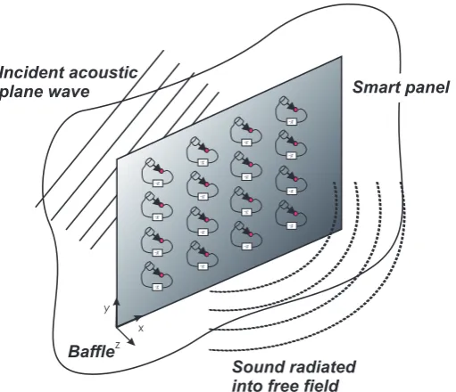
In parallel with the work on ASAC systems with feed-forward control techniques, which are limited to the control of tonal disturbances, work has been carried out to build up ASAC systems where feedback controllers are used. In this case, the reference signal is not required, so these systems can be used to control both tonal and random, wide-band, disturbances. These systems, the signal from the structural sensors are fed back to the structural actuators in such a way as to minimize the vibration component that contributes to the sound radiation. For the case of disturbance rejection feedback control, the most suitable strategy is active damping. This strategy reduces the response of the structure at resonance frequencies. The simplest and most robust way in order to get active damping is by implementing direct velocity feedback (DVFB), in this case the signal from the velocity sensor is directly fed back to the actuators via a fixed control gain. This has led to the design of multichanel feedback controller using state space design [20].

-g

Incident acoustic plane wave

Sound radiated into free field Baffle

y

z x

Smart panel

-g -g

-g

-g -g

-g -g

-g -g

-g -g

-g -g

-g -g

Figure 1.5: Active Structural Acoustic Control (ASAC) with a large number of decentralised collocated sensor-actuators pairs.

1.5 Smart panels for Active Vibration Control (AVC)

frequency averaged kinetic energy and total sound radiation of the panel decreases. This active damping effect on the frequency averaged kinetic energy and total sound power radiation does not grow indefinitely. On the contrary, it tends to decrease for large control gains which tend to pin the structure at the control position. In this way no active damping is injected on the structure. Thus the overall effect is a modification of the spatial response of the structure which becomes pinned at the control position so that, it even radiates more efficiently sound at the new, lightly damped, resonance frequencies.

As shown in Figure 1.5 practical systems can be built using grids of electrodynamic proof mass actuators and closely located accelerometers inertial sensors, as it will be shown later in this thesis. Although these systems are not properly collocated and dual, they enable relatively large feedback control gains, as it will be shown in the chapter 6.

1.6 Sensor-Actuator transducer for smart panels

In the previous sections, the principal features of ASAC and AVC systems have been introduced without taking into account the dynamics of the sensor-actuator transducers used in the smart panels. Therefore, the most common transducers used for the different strategies of active control systems are briefly revised in this subsection.

charge amplifier to the two electrodes. Since these devices have a small mass per unit surface area, they are suited for the construction of distributed sensors.

One way to generate a sky-hook point force on a structure in a smart panel is by means of proof mass electrodynamic actuators [42]. A proof mass actuator can be made with a coil-magnet electrodynamic linear motor, where the coil is fixed to the base or case of the actuator and the magnet is suspended on soft springs so that it provides the inertial reaction necessary to generate a point force on the structure where the proof mass actuator is fixed [19]. These devices will be described in more details later in this thesis. The absolute vibration mode of a structure on a specific point can be measured with inertial accelerometers [38]. This type of devices comprises an elastic transducer with a seismic mass. The transducer normally consists of a piezoelectric element which generates a voltage signal proportional to the relative displacement between the mass and the case respectively. With these devices it is possible to measure the acceleration at a point of a structure provided its natural frequency is well above the measurement range [19].

1.7 Scaling of transducer

In some cases, the scaling of transducers may offer favourable benefits; in fact, smaller devices tend to be faster and consume less power. The smaller they are, the less material is needed in order to be build. They allow new applications where space is confined. As they become smaller, they become portable. Due to batch fabrication technique, they can be mass produced and cost effective. If the production method is compatible with integrated circuit production technique, sensors, actuators, accelerometers and electronics could be integrated on the same chip. By integrating multiple sensors or actuators in one device, reliability can be increased.

When the transducers are scaled down, force, power, speed and other characteristic scale too. However these characteristic do not scale proportionally to the size. Mass and volume, for example, scale with the third power of the size while the surface scales with the second power of the size [43].

1.8 Scope and Objective

The purpose of this thesis is to discuss the design of a light, simple, low cost and robust feedback active control unit to be used in a decentralised MIMO control system arranged on a thin panel in order to control both its vibration and sound radiation. The feedback control unit consists of a proof-mass force actuator with a velocity sensor at its base which implement basic feedback control laws that does not need complex electronic systems to be implemented. The test rig used to study the electrodynamics proof mass actuators consists of a clamped, thin aluminium panel which is excited by either a point force or an acoustic field.

The four main objectives of this thesis are

• to model and study theoretically the stability and control performance properties of one and five feedback control loops on the clamped rectangular panel which, using the velocity error signal, implement [19]:

1. Proportional Control for the implementation of Velocity Feedback; 2. Integral Control for the implementation of Displacement Feedback; 3. Derivative Control for the implementation of Acceleration Feedback and 4. PID Control (Proportional–Integral–Derivative Feedback).

• to study the scaling effects of the actuator with reference to the implementation of velocity feedback control.

• to present stability and control performance experimental test of a miniaturised prototype actuator specifically designed for this study.

1.9 Structure and organisation

This thesis is divided in five chapters. Chapter 2 presents the main features of SISO feedback control on a single degree of freedom system using either an ideal reactive force actuator or a proof mass actuator. The aim of this chapter is twofold. First, to revise the basic stability and control performance properties of Proportional, Integral, Derivative, PI, PD and PID control laws. Second, to investigate the effects on stability and control performance that are produced by the dynamics of a proof mass actuator.

Chapter 3 presents a simulation study about the stability and performance of a control system with five decentralised feedback control units mounted on a flat panel in order to reduce its vibration and sound radiation. Each control unit consists of a proof-mass electro-dynamic actuator with a velocity sensor at its base. The aim is to design light, simple, robust and low cost, control units which can be attached in large numbers to flexible structures in order to control their spatially averaged response and sound radiation at low audio-frequencies. Thus four basic feedback control functions have been studied: a) Proportional, b) Integral c) Derivative and d) PID. Two types of controllers have been considered which drive the actuators either with current or voltage signals.

The study for the various feedback control laws is organised in a consistent framework which first introduces the mathematical model for the various control schemes, it then presents the stability analysis using the Nyquist criterion [19] and finally it gives the control performance results.

The use of proof mass electrodynamic actuators for decentralised velocity feedback control on a rectangular panel is presented in the next two chapters. In chapter 4 the principal features of a small scale proof mass actuator with a low mounting resonance frequency are first presented. In particular a stability–performance formula is derived which can be effectively used to asses the miniaturisation effects on the stability and control performance of the feedback loop. The design and tests of a velocity feedback loop with a prototype miniaturised proof mass actuator are presented in chapter 5.

error signals and five input signals to the amplifiers driving the actuators. The control performance properties have been assessed in terms of the spatially averaged response of the panel measured with a scanning laser vibrometer and the total sound power radiated measured in an anechoic room.

1.10 Contributions

The main original contributions of this thesis are:

• An investigation of the differences feedback control laws using an electrodynamic proof mass actuator which is driven either by current or voltage signals.

• Derivation of a ‘stability–performance’ formula that can be used to assess simultaneously the stability and control performance of the feedback control loop with the proof mass actuator.

• Miniaturisation study of the stability and control performance of a direct velocity feedback loop small scale prototype electrodynamic proof mass actuator mounted on a thin panel.

• Experimental study of stability and control performances of a feedback control unit using a prototype miniaturised proof mass electrodynamic actuator.

2 FUNDAMENTAL CONCEPTS OF FEEDBACK CONTROL

In this chapter, the steady–state response of a Single Degree of Freedom (SDOF) with a reactive point forces or inertial point force feedback control system is studied. First, the response of the SDOF system will be studied when there is no active vibration control assuming different values of damping ratio. Second, the effect of a feedback control loop using either a reactive force actuator or a proof mass force actuator will be examined assuming a small damping ratio. A number of control architectures will be studied namely: a) Proportional Control for implementation of Velocity Feedback, b) Integral Control for implementation of Displacement Feedback c) Derivative Control for implementation of Acceleration Feedback and d) PID Control (Proportional–Integral–Derivative Feedback Control). The aim of this chapter is to introduce the stability and performance analysis of vibration control using proof mass actuators.

2.1 Single degree of freedom system under harmonic motion of the base

Figure 2.1(a) shows the notation used for the mass–spring–dashpot SDOF system under harmonic motion of the base considered in this section.

t

y t( )=Ycosωt System

(a)

Free-body diagram (a)

k x y1( - )1 c x y1( - )1

· ·

m1 m1

k1 c1

x1 x1

Figure 2.1: Single degree of freedom system under harmonic motion of the base.

In this chapter the mechanical kinematics (displacement, velocities, accelerations) or kinetic (force) functions have been taken to be time–harmonic and given by the real part of counterclockwise rotating complex vectors (phasors), so that, for example the displacement

circular frequency [rad/s] and j = −1. Therefore x(t) and f(t) are the time–dependent

harmonic displacement and force function while X(ω) and F(ω) are the complex frequency–dependent displacement and force phasors. In order to simplify the formulation, the harmonic time dependence is assumed in the mathematical expressions. Also, the first and second derivative of the time–harmonic functions will be represented by velocity and

acceleration frequency dependent phasors; X

( )

( )

( )

( )

( )

X =− 2 = _.

Considering the free–body diagram shown in Figure 2.1(b) and using Newton’s second law

of motion (

∑

1 1 1 1 1 1 1 1

m x +c x +k x =c y k y+ (2.1)

where m1 is the proof mass, c1 is the damping coefficient, k1 the stiffness, x1 is the

displacement of the proof mass and the base excitation is given by:

{ }

Re j t

y= Yeω (2.2)

where Y is the amplitude. The right hand side of the Eq. (2.1) base can be seen as a force

f(t) acting on a “classic” SDOF mass–spring–dashpot system with a rigid base:

y k y c

f = 1 + 1 . (2.3)

The steady state solution of Eq. (2.1) can be found by assuming:

( )

{

}

1 1 j t

x t = X e ω . (2.4)

By substituting Eq. (2.4) into Eq. (2.1) and solving for X1, the following relation between the phasors of the mass and base displacement is obtained:

( )

( )

1 2

1 1 1

k jc

X Y

k m j c

ω

ω ω

ω ω

+ =

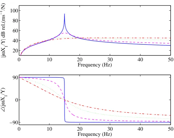
Figure 2.2 shows the variation of the ratio between the velocity of the proof mass and the displacement of the base calculated assuming the physical parameters given in Table 2.1

and for different damping ratios; ξ =c cc where cc is the critical damping:

1

2

c n

c = mω (2.6)

andωnis the natural frequency:

1

1

n

k m

ω = . (2.7)

Table 2.1: Physical parameters for the elements in the SDOF system.

Parameter Value

Critical Damping cc = 2.83 N/ms-1

Mass m1= 0.015 Kg

Stiffness k1= 133.24 N/m

Natural frequency fn = 15 Hz

0 10 20 30 40 50

20 40 60 80 100

Frequency (Hz)

|j

ω

X 1

/Y| dB rel.(ms

−1

/N)

0 10 20 30 40 50

−90 0 90

Frequency (Hz)

∠

(j

ω

X 1

/Y)

The key features of the SDOF system under study can summarised in the following points:

• For an undamped system (ξ=0) |jωX1/Y| tends towards infinity at resonance.

• The addition of small amounts of damping lead to important reductions of the response at, or near, resonance but also increase the response at frequencies much higher than resonance.

• Increasing damping causes the frequency of maximum response to move to lower values.

• Increasing the amount of damping leads to a smoother phase transition.

The results shown in Figure 2.2 indicate that, in order to obtain the maximum vibration reduction of the mass, the spring element should be selected in such a way as to keep the natural frequency as low as possible in respect to the limitation imposed on the static displacement δ = m1g/ k1, where g is the acceleration due to the gravity, which also depends on the stiffness of the spring. Also the damping effect should be as small as possible, although also in this case a compromise must be found in order to avoid excessive vibrations transmission around the resonance frequency.

2.2 SDOF system under harmonic motion of the base with a reactive force feedback control loop

The design problems highlighted above generate important limitations to the low frequency passive isolation effect introduced by the spring–dashpot element. An interesting and effective way to enhance the vibration isolation is the implementation of an active control system.

t

y t( )=Ycosωt System

(a) Free-body diagram

(a)

k x y1( - )1 c x y1( - )1

· ·

m1

x1

m1

k1 c1

Fc

Fc

x1

~

H( )ω

Fc

In this section the effects produced by a feedback control system, which, as shown in Figure 2.3(a), is composed by a) a control sensor that measures the velocity of the mass, b) a control actuator mounted in parallel with the spring–dashpot elements that produces reactive forces between the mass and base and c) a control system that implement a control function –H which in the simplest case is given by a pure gain; –g.

The equation of motion for the system shown in Figure 2.3(a) with a Proportional, Integral, Derivative, or combination among the three control functions can be derived from the free-body diagram shown in Figure 2.3(b) using Newton’s second law of motion, which gives:

1 1 1 1 1 1 1 1 c

m x +c x +k x =c y k y+ + f (2.8)

where Re{ j t}

c c

f = F eω is the feedback reactive control force which depends on the control

loop used as it is described in the sections below:

2.2.1 Proportional control for implementation of velocity feedback

In this case, the output signal from the velocity sensor is feedback to the actuator via a negative proportional function, i.e. H(ω)=-gP, where gP is a fixed proportional gain, so that the phasor of the control force Fc, is directly proportional to the opposite of the velocity of the mass:

( )

c P

F = −g X ω . (2.9)

Therefore substituting the steady state solution ₁

( )

x t = X eω (Eq.(2.4)) into the equation of motion (Eq.(2.1)), with _y=Yejωt, _and

( )

1

c P

F = −g X ω , the following expression for the complex amplitude of the response is obtained:

( )

₍

_{) ( )}

1 2

1 1 1

P

P

k jc

X Y

k m j c g

ω

ω ω

ω ω

−

+ =

− + + (2.10)

2.2.2 Integral control for implementation of displacement feedback

In this case, the output signal from the velocity sensor is feedback to the actuator via a negative integral control function, i.e. H(ω)=–gI/jω, where gI is a fixed integral gain, so that the phasor of the control force Fc is directly proportional to the opposite of the displacement of the mass. Hence Fc is given by:

( )

_{( )}

1

1

c I I

X

F g g X

j ω

ω ω

= − = − . (2.11)

Following the same procedure as in the previous subsection, the complex response is found to be in this case:

( ) (

)

( )

1 2

1 1 1

I

I

k jc

X Y

k g m j c

ω

ω ω

ω ω

−

+ =

+ − + . (2.12)

The denominator indicates that Integral Control adds active stiffness so that the resonance frequency is moved to higher values as it will be further discussed in section 2.4.

2.2.3 Derivative control for implementation of acceleration feedback

In this case, the output signal from the velocity sensor is feedback to the actuator via a derivative control function, i.e. H(ω)=–gDjω, where gD is a fixed derivative gain, so that the phasor of the control force Fc, is directly proportional to the opposite of the acceleration of the mass. Hence Fc is given by:

( )

( )

1 1

c D D

F = −j g Xω ω = −g X ω . (2.13)

Once more, following the procedure highlighted in the previous subsections the response is found to be:

( )

₍

₎

( )

1 2

1 1 1

D

D

k jc

X Y

k m g j c

ω

ω ω

ω ω

−

+ =