Graceful Trees: Statistics and Algorithms

(1)

Graceful Trees: Statistics and

Algorithms

By Michael Horton, BComp

A dissertation submitted to the

School of Computing

in partial fulfilment of the requirements for the degree of

Bachelor of Computing with Honours

School of Computing University of Tasmania

(2)

Statement

I, Michael Horton do hereby declare that this thesis contains no material that has been accepted for the award of any other degree or diploma in any tertiary institution. To the best of my knowledge and belief it contains no material previously published by another person, except where due reference is made in the text of the thesis.

(3)

Abstract

(4)

List of tables

Table 3-1: RANRUT mean running time per tree, for 256 trees of each size... 17

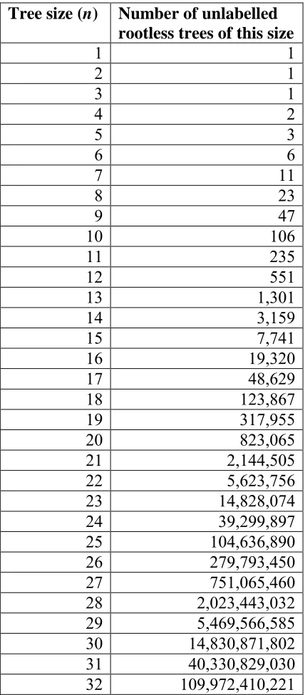
Table 5-1: The number of unlabelled rootless trees on 1 to 32 nodes (Otter 1948)... 48

Table 6-1: Comparison of the best case proportion of labellings that are graceful with the 1-star ... 60

Table 6-2: Comparison of the worst case proportion of labellings that are graceful with the chain ... 61

Table B-1: EdgeSearchBasic running time ... 75

Table B-2: EdgeSearchBasic calls to FindEdge ... 75

Table B-3: EdgeSearchRestart running time ... 76

Table B-4: EdgeSearchRestart calls to FindEdge... 76

Table B-5: EdgeSearchRestartMirrors running time ... 77

Table B-6: EdgeSearchRestartMirrors calls to FindEdge ... 77

Table B-7: EdgeSearchRestartMirrors running time for random trees... 78

Table B-8: EdgeSearchRestartMirrors calls to FindEdge for random trees ... 79

Table B-9: Worst-case running times of the three edge search algorithms ... 80

Table B-10: Mean running times of the three edge search algorithms ... 80

Table B-11: Worst-case calls to FindEdge for the three edge search algorithms... 81

Table B-12: Mean calls to FindEdge for the three edge search algorithms... 81

Table C-1: Counts of graceful labellings/all possible labellings for all trees on 1-9 nodes. This is the first part of the table containing proportions for all trees on 1-12 nodes. ... 82

Table C-2: The proportion of all possible labellings that are graceful for all trees on 1-9 nodes. This is the first part of the table containing proportions for all trees on 1-12 nodes. ... 83

Table C-3: Log to base n of the proportion of all possible labellings that are graceful for all trees on 1-9 nodes ... 84

Table C-4: Averages of the proportion of all possible labellings that are graceful for all trees on 1-12 nodes ... 85

(7)

List of figures

Figure i: Example of a graph, with 8 vertices and 9 edges... x

Figure ii: Example of a tree, with 7 vertices and 6 edges ... x

Figure iii: K6, the complete graph with 6 vertices and 15 edges ... xi

Figure iv: A rooted tree, showing the level of each vertex ...xiii

Figure v: Arithmetic and logarithmic scales ... xiv

Figure vi: Example of mirrored nodes – the 2, 3 and 4 can be rearranged at will... xiv

Figure 2-1: An example of a gracefully labelled tree... 2

Figure 2-2: The 5-node chain, gracefully labelled by Cahit and Cahit’s algorithm ... 3

Figure 2-3: A caterpillar, gracefully labelled by Cahit and Cahit's algorithm. The upper horizontal line is the chain section; only paths of length 1 may be attached to it... 3

Figure 2-4: A 2-star, gracefully labelled by Cahit and Cahit's algorithm ... 3

Figure 2-5: The k=3 olive tree... 4

Figure 2-6: A banana tree constructed from a 2-star, 3-star and 1-star... 4

Figure 2-7: Rearranging a gracefully labelled path to generate a gracefully labelled Tp-tree... 5

Figure 2-8: Example of a graceful product tree... 6

Figure 2-9: K7 being decomposed into 7 isomorphic trees of size 3... 9

Figure 2-10: Example of a gracefully labelled graph... 10

Figure 2-11: A graph that cannot be gracefully labelled... 11

Figure 2-12: A harmoniously labelled graph... 11

Figure 2-13: A harmoniously labelled tree ... 11

Figure 2-14: A cordially labelled graph ... 12

Figure 2-15: A cordially labelled tree ... 12

Figure 2-16: K4: A graph that cannot be cordially labelled ... 12

Figure 3-1: The primary canonical level sequences and resulting trees drawn by successive calls to NextTree for n=6... 15

Figure 4-1: The edge search starts by testing node label 1 on the first node. All nodes adjacent to the labelled node are marked possible. ... 21

Figure 4-2: The first edge label to be considered is 4. It is tested on the first possible node. Since the node above the possible node is labelled 1, a node label of -3 or 5 is required to achieve this. Only 5 lies within the bounds of the possible node labels, so it is applied. ... 21

Figure 4-3: Whenever a possible node is labelled, all unlabelled adjacent nodes are marked possible. ... 21

Figure 4-4: The initial search gets this far but can’t find any way to obtain edge label 1, so it backtracks... 22

Figure 4-5: The next recursion tries edge label 2 on the bottom node but has no better luck. .... 22

Figure 4-6: Since edge label 3 to the centre node failed, it’s tried to the right-hand node. ... 22

Figure 4-7: This time, edge labels 2 and 1 follow easily and a graceful labelling is recorded. ... 22

Figure 4-8: Chart showing how mean calls to FindEdge is closely correlated to mean running time. Both scales are logarithmic. ... 24

Figure 4-9: Chart showing how worst-case calls to FindEdge is closely correlated to worst-case running time. Both scales are logarithmic. ... 25

Figure 4-10: Basic edge search algorithm worst-case running time (arithmetic scale) ... 25

Figure 4-11: Basic edge search algorithm mean running time (arithmetic scale)... 26

Figure 4-12: Basic edge search algorithm worst-case and mean running time (logarithmic scale) ... 26

Figure 4-13: Basic edge search algorithm worst-case calls to FindEdge (arithmetic scale) ... 27

Figure 4-14: Basic edge search algorithm mean calls to FindEdge (arithmetic scale)... 27

Figure 4-15: Basic edge search worst-case and mean calls to FindEdge (logarithmic scale) ... 28

Figure 4-16: EdgeSearchRestart worst-case running time (arithmetic scale)... 30

Figure 4-17: EdgeSearchRestart mean running time (arithmetic scale) ... 30

Figure 4-18: EdgeSearchRestart worst-case and mean running time (logarithmic scale) ... 31

Figure 4-19: EdgeSearchRestart worst-case calls to FindEdge (arithmetic scale)... 31

Figure 4-20: EdgeSearchRestart mean calls to FindEdge (arithmetic scale) ... 32

Figure 4-21: EdgeSearchRestart calls to FindEdge (logarithmic scale) ... 32

Figure 4-22: EdgeSearchRestartMirrors worst-case running time (arithmetic scale) ... 33

Figure 4-23: EdgeSearchRestartMirrors mean running time (arithmetic scale)... 33

(8)

Figure 4-25: EdgeSearchRestartMirrors worst-case calls to FindEdge (arithmetic scale) ... 34

Figure 4-26: EdgeSearchRestartMirrors mean calls to FindEdge (arithmetic scale)... 35

Figure 4-27: EdgeSearchRestartMirrors worst-case and mean calls to FindEdge (logarithmic scale) ... 35

Figure 4-28: EdgeSearchRestartMirrors worst-case running time for random trees (arithmetic scale) ... 36

Figure 4-29: EdgeSearchRestartMirrors mean running time for random trees (arithmetic scale) ... 36

Figure 4-30: EdgeSearchRestartMirrors worst-case and mean running time for random trees (logarithmic scale) ... 37

Figure 4-31: EdgeSearchRestartMirrors worst-case calls to FindEdge for random trees (arithmetic scale) ... 37

Figure 4-32: EdgeSearchRestartMirrors mean calls to FindEdge for random trees (arithmetic scale) ... 38

Figure 4-33: EdgeSearchRestartMirrors worst-case and mean calls to FindEdge for random trees (logarithmic scale)... 38

Figure 4-34: Worst-case running time for the three forms of EdgeSearch ... 39

Figure 4-35: Mean running time for the three forms of EdgeSearch... 39

Figure 4-36: Worst-case calls to FindEdge for the three forms of EdgeSearch ... 40

Figure 4-37: Mean calls to FindEdge for the three forms of EdgeSearch ... 40

Figure 4-38: Example of a graceful labelling not covered by the edge search conjecture... 41

Figure 4-39: This shows the difference between IdenticalNode and NodeSet. All nodes marked with an ‘I’ are identical for the purposes of starting nodes, but only those marked with an ‘S’ are part of the same set when FindEdge is running. ... 42

Figure 4-40: The 29-node tree 5,469,558,977, an example of a tree that the edge search algorithm finds difficult... 46

Figure 6-1: Example of the labellings considered by the statistical analysis ... 52

Figure 6-2: Chart of the total number of labellings that are graceful for all trees on 1 to 12 nodes (arithmetic scale) ... 53

Figure 6-3: Chart of the total number of labellings that are graceful for all trees on 1 to 12 nodes (logarithmic scale) ... 54

Figure 6-4: Chart of the mean of the total graceful labellings for all trees on 1 to 12 nodes (logarithmic scale) ... 54

Figure 6-5: Chart of the proportions of all possible labellings that are graceful for all trees on 1-12 nodes (arithmetic scale) ... 55

Figure 6-6: Chart of the proportions of all possible labellings that are graceful for all trees on 1-12 nodes (logarithmic scale) ... 56

Figure 6-7: Chart of the arithmetic mean of the proportion of all possible labellings that are graceful (logarithmic scale) ... 56

Figure 6-8: Chart of the geometric mean of the proportion of all possible labellings that are graceful (logarithmic scale) ... 57

Figure 6-9: Chart of logn of the proportions of all possible labellings that are graceful, including the arithmetic mean of the logs ... 58

Figure 6-10: Arithmetic mean of the logn (proportion of all possible labellings that are graceful), with linear trendline fitted; the error bars show one standard deviation ... 58

Figure 6-11: Chart of the proportion of all possible labellings that are graceful, including the maximum and minimum for each tree size... 59

Figure 6-12: The proportion of all labellings that are graceful with maxima and minima, on a logarithmic scale... 59

Figure 6-13: Structure of the n-node 1-star... 60

Figure 6-14: Structure of the n-node chain ... 61

Figure 6-15: The proportion of all labellings that are graceful with maxima, minima and 1-star and chain proportions added (logarithmic scale) ... 61

Figure 6-16: The 5-node chain with an additional edge one segment from the end admits 360 labellings, 6 of which are graceful (proportion=0.0167) ... 62

Figure 6-17: The 5-node chain with an additional edge in the centre admits 360 labellings, 8 of which are graceful (proportion=0.0222)... 62

(9)

Acknowledgements

I would like to acknowledge the valuable assistance of Dr Francis Suraweera, my supervisor. Without him I wouldn’t even know what a graceful tree is, which would be a terrible shame.

(10)

Definitions

In this thesis, we use standard graph terminology. The reader is referred to the standard textbooks by Bollobás (Bollobás 1979) and Harary (Harary 1972).

Graph

[image:10.595.129.301.557.674.2]

A graph, in the context of this thesis, is a mathematical construct containing points (called ‘vertices’) connected by line segments (‘edges’) (Bollobás 1979 p1). An example graph is shown in Figure i.

Figure i: Example of a graph, with 8 vertices and 9 edges

Tree

A tree is a specialised form of graph. In a tree, every pair of vertices must be connected by one, and only one, set of edges (Bollobás 1979 p5). The example graph in Figure i is not a tree, because the two vertices on the right are not connected at all, while the vertices on the left are connected to each other through several paths. A correct example of a tree is shown in Figure ii. If the connection requirement is to be satisfied, a tree with n vertices must have n-1 edges. The only exception to these rules is the empty tree, which has no vertices and no edges.

Figure ii: Example of a tree, with 7 vertices and 6 edges

(11)

Adjacency

Two vertices are adjacent if they share an edge (Bollobás 1979 p1).

Complete graph

A complete graph has one edge from every vertex to every other vertex. The complete graph with n vertices is represented by the symbol Kn. and will have

(n(n-1))/2 edges (Figure iii) (Bollobás 1979 p3).

Figure iii: K₆, the complete graph with 6 vertices and 15 edges

Degree

The degree of a vertex in a graph is the number of vertices adjacent to it (Bollobás 1979 p3).

Degree sequence

The degree sequence of a graph is a sequence listing the degree of every vertex. For graphs, the ordering is arbitrary; for trees, the ordering is given by a pre-order traversal, starting from an arbitrary node. For the tree in Figure ii, three equally valid degree sequences are {1, 3, 1, 4, 1, 1, 1}, {1, 3, 4, 1, 1, 1, 1} and {4, 3, 1, 1, 1, 1, 1}. Only one tree can satisfy a degree sequence definition, however.

Diameter

To find the diameter of a graph, first find the distance between every pair of vertices. The diameter is the maximum of these minima (Bollobás 1979 p8). The diameter of a tree is much simpler; as there is always one and only one path of edges between any two vertices, there is only one possible distance. The diameter of the tree in Figure ii is 3; the diameter of the graph in Figure iii is 1.

Distance

(12)

Mean

‘Mean’ without an adjective implies the arithmetic mean (see below.)

Mean, arithmetic

The arithmetic mean of a set of numbers is their sum divided by their count. For example,

ArithmeticMean([1, 2, 4, 5]) =(1+2+4+5)/4

=12/4 =3

Mean, geometric

The geometric mean of a set of n numbers is the nth root of their product. It is more commonly calculated by taking the exponent of the arithmetic mean of their natural logs. The geometric mean is not as vulnerable to high-valued outliers as the arithmetic mean and may be more appropriate for highly skewed distributions. As an example,

GeometricMean([1, 2, 4, 5])

=e^(ArithmeticMean([ln(1), ln(2), ln(4), ln(5)])) =e^(ArithmeticMean(0.000, 0.693, 1.386, 1.609)) =e^(0.922)

=2.515

Isomorphic

Two graphs are isomorphic if they have the same structure – if, by rearranging their vertex identification, they can be shown to share the same set of edges (Bollobás 1979 p3).

Level

The level of vertices is only meaningful for rooted trees. The level of a vertex is the distance from it to the root. The level of the root is zero (Wright et al. 1986).

Level sequence

(13)

may happen in any order. One possible level sequence for the tree in Figure iv is {0, 1, 2, 2, 2, 1, 1}. Each level sequence does describe a single tree.

Figure iv: A rooted tree, showing the level of each vertex

Lexicographic order

Lexicographic order is a common way to compare sequences; it is used in dictionaries to order words, which are sequences of letters (Aho & Ullman 1995 p29). For two sequences A and B, A is less than B in lexicographic order if:

1. A is a prefix of B

or

2. For some integer i, A1…i-1≡B1…i-1 and Ai<Bi

Logarithmic scale

Logarithmic scales are a useful way to chart numbers that increase or decrease exponentially. The chart scale increases exponentially (usually by a multiple of 10) so that any value that increases exponentially will form a straight line. A disadvantage is that, because logarithms are only defined for positive numbers, only positive values can be displayed on a logarithmic scale. The difference between arithmetic and logarithmic scales is illustrated in Figure v.

0

1 1 1

(14)

0 10 20 30 40 50 60 70 80 90 100

1 6

x

y y=x!

y=3^x y=2^x y=x

1 10 100 1000

1 6

x

y y=x!

y=3^x y=2^x y=x

Figure v: Arithmetic and logarithmic scales

Node

A node is another name for a vertex. Within this thesis ‘node’ and ‘vertex’ are used interchangeably.

Node, Mirrored

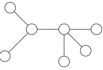
All of the work in this thesis is related to trees with labelled nodes. ‘Mirror Nodes’ are a concept created to describe sets of nodes that do not need to have all possible labellings tested because they are part of identical structures. For example the three trees in Figure vi are structurally identical. This means that any algorithm that looked at all three would be wasting time on the second two.

Figure vi: Example of mirrored nodes – the 2, 3 and 4 can be rearranged at will

Two nodes n1 and n2 are considered mirrored if:

1. The rooted tree with n1 as the root is isomorphic to the rooted tree

with n2 as the root

2. n1 and n2 are adjacent or are adjacent to a common node

… 1

5

2 3 4

6

1 5

4 3 2

6

1 5

2 4 3

(15)

1 Introduction

A tree with n vertices is ‘gracefully labelled’ if its vertices can be labelled with the integers [1..n], using each once and only once, such that its edges, when labelled with the difference between the endpoint vertex labels, are labelled with the integers [1..n-1], with each number used once and only once. If a tree can be gracefully labelled, it can be called a ‘graceful tree’ (Rosa 1967).

The ‘Graceful Tree Conjecture’, or ‘Ringel-Kötzig Conjecture’, states that all trees are graceful (Gallian 2000). It has not been proven, although some specialised classes of tree can be shown to always be graceful (Cahit & Cahit 1975; Pastel & Raynaud 1978; Hrnciar & Havier 2001; Koh et al. 1980). Computer searches have also been used to show that all trees with up to 28 vertices are graceful (Aldred & McKay 1998; Nikoloski et al. 2002). Although searches to finite sizes can never prove the conjecture true, they may be able to prove it false. They also pose an intriguing problem in algorithm design, as the exhaustive search demands a very fast graceful labelling algorithm.

Statistical techniques can also help us estimate trends in graceful labellings, by showing how the total number of labellings, and the proportion of labellings that are graceful, change as tree size increases. In particular, statistical trends can suggest if we can expect that at some large number of vertices a non-graceful tree will be found.

This thesis describes the development of a new graceful labelling algorithm, adjustments to improve its running time and its use to prove that all trees with 29 vertices are graceful.

Trends are also found in the statistics of small graceful trees and some future research directions are proposed.

(16)

2 Literature Review

2.1 The Graceful Tree Conjecture

A tree with n vertices is said to be gracefully labelled if its vertices are labelled with the integers [1..n] such that the edges, when labelled with the difference between their endpoint vertex labels, are uniquely labelled with the integers [1..n-1] (Figure 2-1).

Figure 2-1: An example of a gracefully labelled tree

If a tree can be gracefully labelled, it is called a ‘graceful tree.’ The concept of graceful labelling of trees and graphs was introduced by Rosa (Rosa 1967) and named a ‘β-valuation.’ The term ‘graceful labelling’ was invented by Golomb (Golomb 1972).

The ‘Graceful Tree Conjecture,’ (also known as the ‘Ringel-Kötzig Conjecture’ (Gallian 2000)) suggests that all trees are graceful. So far, no proof of the truth or falsity of the conjecture has been found. In the absence of a generic proof, two approaches have been used in investigating the graceful tree conjecture: proving the gracefulness of specialised classes of tree, and exhaustively testing trees up to a specified size for graceful labellings. Both of these approaches are investigated here, along with some of the related problems in the wider field of graph labelling.

2.2 Approach 1: Classes of graceful tree

Some types of trees have been shown to be always graceful. Many of the proofs that all trees of a pattern are graceful are also ‘constructive,’ and provide a guaranteed labelling method for trees that follow that pattern.

1

5 6

2 3

5 4

3

(17)

2.2.1 Chains

A chain (or ‘path’), is the simplest type of tree: a single line of vertices (Figure 2-2). A chain is a caterpillar (see below) with no legs; chains can always be labelled by Cahit and Cahit’s caterpillar-labelling algorithm (Cahit & Cahit 1975).

Figure 2-2: The 5-node chain, gracefully labelled by Cahit and Cahit’s algorithm

2.2.2 Caterpillars

A caterpillar is a tree with one long chain of vertices and any number of paths of length 1 attached to the chain (Figure 2-3). Cahit and Cahit created a constructive proof that all caterpillars (which they call ‘string trees’) are graceful (Cahit & Cahit 1975).

Figure 2-3: A caterpillar, gracefully labelled by Cahit and Cahit's algorithm. The upper horizontal line is the chain section; only paths of length 1 may be attached to it.

2.2.3 m-stars

An m-star has a single root node with any number of paths of length m attached to it

(Figure 2-4). Cahit and Cahit also proved that all m-stars a graceful (Cahit & Cahit 1975).

Figure 2-4: A 2-star, gracefully labelled by Cahit and Cahit's algorithm 9

1

3 6

2 8

5 2

8

5 7

5 1 7

4 3

6

1

14

7 8

6 13

4 11

3

11 10 9

12

2

13 5

12

10

6

4 2

8 7

9 1 5 3

(18)

2.2.4 Trees with diameter five

The diameter of a graph or tree is the maximum of the shortest paths between its vertices (Bollobás 1979). Hrnciar and Havier extended the proof for caterpillars to show that all trees with diameter≤5 are graceful (Hrnciar & Havier 2001).

2.2.5 Olive trees

An olive tree has a root node with k branches attached; the ith branch has length i (Figure 2-5). Pastel and Raynaud proved that all olive trees are graceful (Pastel & Raynaud 1978).

Figure 2-5: The k=3 olive tree

2.2.6 Banana trees

A banana tree is constructed by bringing multiple stars together at a single vertex (Chen et al. 1997) (Figure 2-6). Banana trees have not been proved graceful, although Bhat-Nayak and Deshmukh have proven the gracefulness of certain classes of banana tree (Bhat-Nayak & Deshmukh 1996).

(19)

2.2.7 Tp-Trees

Hegde and Shetty defined a class of tree called ‘Tp-trees’ (transformed trees) created by taking a gracefully labelled chain and shifting some of the edges (Figure 2-7), and proved that they can always be gracefully labelled using the original chain labels (Hegde & Shetty 2002).

Figure 2-7: Rearranging a gracefully labelled path to generate a gracefully labelled Tp-tree

2.2.8 Product trees

Some proofs also show that certain graceful trees can be added together to give a larger graceful tree. Koh et al. show how ‘rooted product’ trees are always graceful (Koh et al. 1980). An example from their paper is given in Figure 2-8. Each of the trees labelled G shares one vertex with the tree labelled H.

3

7 3

5 8

4 2

6 2

6 4

5 1

9 8 1 3

7 3

5 8

4 2

6 2

6 4

5 1

9 8 1

(20)

Figure 2-8: Example of a graceful product tree

2.3 Approach 2: Exhaustive labelling

The graceful tree conjecture may be wrong. If so, the simplest proof would be to find a counterexample – a tree that cannot be gracefully labelled. So far, however, searches have merely found billions of graceful trees, giving additional credence to the conjecture without formal proof. These currently cover every tree with up to 28 vertices (Aldred & McKay 1998; Nikoloski et al. 2002).

2 3 1

5 4 H 1 6 2 5 3 4 3 4 5 1 2 6 1 6 2 5 3 4 5 4 3 1 6 2

G2 G3 G4

(21)

To run an exhaustive test requires two algorithms: one that finds graceful labellings, and one that draws every tree of the requested size. Both algorithms must be as efficient as possible, as the running time limits the size that may be searched to.

2.3.1 Graceful labelling algorithms

2.3.1.1 Exhaustive labelling algorithms

The simplest algorithm to write is to try all n! vertex labellings. This will execute in O(n!) time, and rapidly becomes impractical as n increases. This algorithm is not fast enough to test one tree of size 29, to say nothing of every possible tree of size 29. It does have the advantage that it will find not just one graceful labelling but every possible labelling. This makes it useful for statistical analysis at small sizes.

2.3.1.2 Forward-thinking labelling algorithms

Exhaustive searches can easily find themselves in dead-end states without noticing. For example, the tree must include edge label n-1. This can only be found between the vertex labels 1 and n, which therefore must be adjacent to each other. If they aren’t, the tree cannot possibly be labelled gracefully, and testing labels on the rest of the tree will merely waste time. Nikoloski et al. found an algorithm that uses a triangular tableau to identify and ignore cases of this type (Nikoloski et al. 2002).

2.3.1.3 Approximation labelling algorithms

Hill-climbing techniques have also been effective; one was used in Aldred and McKay’s exhaustive search to n=27 (Aldred & McKay 1998). The general idea is that any modification to the vertex labels that increases the number of unique edge labels moves closer to a solution, so is a move up the hill. However, approximate answers are not sufficient where graceful labellings are concerned. If the hill-climbing finds itself stuck without reaching n-1 unique edge labels, it must be started over. The need to restart keeps the hill-climbing technique at exponential efficiency. To keep this thesis self-contained, Aldred and McKay’s algorithm is described below.

Graceful and Harmonious alg.

For a given tree T and labelling L of the vertices, let

(22)

For n=|V(T)|, the aim is to find L such that z(T,L)=n-1.

If L is a labelling and v,w∈V(T), define Sw(L;v, w) to be

the labelling got from L by swapping the labels on v and

w.

Using a parameter M:

1. Start with any labelling of V(T).

2. If z(T,L)=n-1, stop.

3. For each pair {v, w}, replace L by L’=Sw(L;v, w)

if z(T,L’)>z(T, L).

4. If step 3 finishes with L unchanged, replace L by

Sw(L;v, w), where {v, w} is chosen at random from

the set of all {v, w} such that

(a) {v, w} has not been chosen during the most

recent M times this step has been executed.

(b) Sw(L;v, w) is maximal subject to (a).

5. Repeat from step 2.

One part of this algorithm that can be adjusted is the value of M. Aldred and McKay report that “A value of M=10 seems ok for small trees, but a slightly larger value seems to be needed for larger trees. The purpose of M is to prevent the algorithm from repeatedly cycling around within some small set of labellings” (Aldred & McKay 1998).

2.3.2 Tree construction

2.3.2.1 Constructing all trees

To test every tree with n nodes for a graceful labelling, as Aldred and McKay did, requires that every tree with n nodes be drawn. Their paper suggests Wright et al.’s NextTree algorithm (Wright et al. 1986). If NextTree is started with the n-node chain and called repeatedly, it will draw every unlabelled rootless tree, without duplicates.

2.3.2.2 Constructing random trees

(23)

unfeasible. The next best alternative is to test the algorithm on an evenly distributed random sample.

To generate evenly distributed random rootless unlabelled trees we adapted the algorithm ‘RANRUT’ proposed by Nijenhuis and Wilf (Nijenhuis & Wilf 1978), which generates random rooted unlabelled trees. In their paper, they give the algorithm’s FORTRAN source code. For completeness, it is included in appendix A.

2.4

2.5 Summary

The graceful tree conjecture has yet to be proven. Specialised proofs show that limited types of trees are graceful for all sizes, while exhaustive searches show that limited sizes of tree are graceful for all types.

The exhaustive search approach has also given rise to the field of graceful labelling algorithms, which are an interesting problem in algorithm design.

(28)

3 Methods

3.1 Introduction

In order to carry out an exhaustive labelling of every tree with 29 nodes, it is necessary to actually draw the trees. Sometimes, however, drawing every tree is impractical – when analysing an algorithm’s running time on 40-node trees, for example. The algorithm may instead be tested on a random sample of 40-node trees.

3.2 Drawing every size

n

tree

Several parts of this investigation required that every n-node tree be drawn. In particular, all trees with 29 nodes were tested to see if they admitted a graceful labelling. There are 5,469,566,585 such trees (Otter 1948); to generate all of them in reasonable time is not a trivial exercise. NextTree, an efficient algorithm that draws all trees of size n with constant time per tree and O(n) space (Wright et al. 1986) was chosen. The pseudocode of NextTree is given in appendix A.

3.2.1 Encoding the trees

This algorithm uses a tree encoding called the primary canonical level sequence. This extends the notion of a canonical level sequence, which is discussed by Beyer and Hedetniemi (Beyer & Hedetniemi 1980) to draw all unique n–node rooted trees. The canonical level sequence of a tree is the distance of every node from the root, sequenced by a pre-order traversal that visits subtrees in nonincreasing lexicographic order. The primary canonical level sequence is a canonical sequence rooted at the centre of the tree. For trees with two centre nodes, the root with fewer nodes on its side of the centre is chosen. If both potential roots have the same number of nodes, the root that generates a lexicographically smaller canonical level sequence is chosen. If the canonical level sequences are identical, both roots would generate the same primary canonical level sequence, so choice of root is irrelevant.

3.2.2 Generating the trees

(29)

of every unique n-node rootless tree, finishing with the size n 1-star. An example of the trees it draws, in order, is given in Figure 3-1.

Figure 3-1: The primary canonical level sequences and resulting trees drawn by successive calls to NextTree for n=6

The NextTree algorithm generated all 5,469,566,585 trees with 29 nodes within 10 minutes on a 2.4 GhZ Pentium IV. Testing every tree for a graceful labelling would take a little longer. Specifically, it took 58 days. The running time may therefore be considered negligible compared to the labelling time.

3.3 Drawing random size

n

trees

Some of the algorithm runtime analysis had to be run without a full set of trees. Instead, it was tested on a random sample, which should be as evenly distributed as

Tree 1

Level sequence=1 2 3 3 2 3 Tree 0

Level sequence=1 2 3 4 2 3

Tree 2

Tree 3

Tree 4

Tree 5

(30)

possible – if the random sample is biased in favour of some pattern of trees, the running time will be inaccurate.

(The computers used in this research were not able to generate truly random numbers, so the algorithms as implemented could only generate pseudorandom trees.)

3.3.1 Simple random tree construction

Constructing random trees is quite simple if the problem of distribution is ignored. For the initial tests, the following algorithm was used:

Algorithm ConstructRandomTree

Input: Random number seed, size

Output: A random tree of appropriate size

Variables: parent, an array[0..size-1] of integer. This

stores the parent of each node. A parent of -1 indicates

that the node has no parent (it is the root.)

parent[0]<- -1

For every node i from 1 to size-1

parent[i]<-random(0..i-1)

This may generate every unlabelled tree with size nodes, but the distribution will not be even.

3.3.2 Evenly distributed random tree construction

3.3.2.1 Random rooted unlabelled trees

For more robust results, the RANRUT algorithm written by Nijenhuis and Wilf (Nijenhuis & Wilf 1978) was chosen. The complete FORTRAN source written by Nijenhuis and Wilf is included in appendix A. RANRUT generates an even distribution of random unlabelled rooted trees.

3.3.2.2 Random rootless unlabelled trees

(31)

nodes with the equal greatest degree sequence-1) returned zero. These changes meant that the algorithm generated an even distribution of random unlabelled rootless trees as required. This adaption worked, although it was quite slow (Table 3-1).

Tree size Mean drawing time (s)

4 0.000730

8 0.004762

12 0.018129

16 0.045531

20 0.088258

24 0.030945

28 0.012570

32 0.016297

Table 3-1: RANRUT mean running time per tree, for 256 trees of each size

The random rootless tree drawing algorithm was still capable of generating trees for run time analysis at sizes that were too large for exhaustive testing with NextTree.

(32)

4 The edge search algorithm

4.1 Introduction

The simplest approach to writing a graceful labelling algorithm is to concentrate upon fitting node labels into the tree. However, another possibility is to concentrate on fitting the edge labels, while making sure that no invalid node labels are used. This possibility inspired the edge-based depth-first search graceful labelling algorithm described here.

The edge search algorithm applies the edge labels in sequence, starting with edge label n-1, then putting edge n-2 adjacent to that, then n-3 adjacent to one of the existing edges, continuing until edge label 2 and edge label 1 are applied. Edge search assumes that a graceful labelling exists where every edge smaller that n-1 can be fitted adjacent to an edge with a greater label. This leads to a conjecture that is discussed in section 4.5.

Edge search has some similarities with an unpublished algorithm by Suraweera and Anderson (Suraweera & Anderson 2002) which analyses the degree sequence and fits edges around it.

The data found for the running time analyses in this chapter are listed in appendix B.

4.2 The basic algorithm (EdgeSearchBasic)

Although it was expanded in several ways, the edge search algorithm started like this:

Algorithm EdgeSearchBasic

Input:

T, a rootless tree that stores adjacency lists for every

node.

Output:

A graceful labelling for the input tree.

(33)

Size, the size of the tree

Possible, an array of Booleans storing which nodes are

candidates for edge labelling

Procedure search

For every possible starting node from 0 to size-1

Set all nodes impossible

Set the label of the starting node to 1

Record that all nodes adjacent to the starting

node are possible

FindEdge(Size-1)

End for

End procedure

Procedure FindEdge

Input:

EdgeLabel, the edge currently being searched for

T, a rootless tree with a spanning tree of edge labels

from Size to EdgeLabel+1

Output:

A graceful labelling of T, if one was found.

Variables:

PossibleNode, a node found on the possible list

PreviousNode, the labelled node above PossibleNode

LowLabel & HighLabel, the two possible node labels that

could be used to achieve EdgeLabel on the edge between

PreviousNode and PossibleNode

TestLabel, the node label decided upon

If EdgeLabel=0 then

Record labelling found

Else

(34)

PossibleNode←the possible node

PreviousNode←the node above PossibleNode

LowLabel←PreviousNode’s label-EdgeLabel

HighLabel←PreviousNode’s label+EdgeLabel

If LowLabel or HighLabel are within the

range 1..size and have not already been

used then

TestLabel←the potential label

NodeLabel[PossibleNode]<TestLabel

Record that PossibleNode now has

label TestLabel

Record that the node label TestLabel

has been used

Set PossibleNode impossible

Set all nodes adjacent to

PossibleNode possible

FindEdge(EdgeLabel-1)

Restore the state before this

labelling was tried (set all adjacent

nodes impossible, set PossibleNode

back to possible and record that node

label TestLabel may be used again.)

End if

End for

End else

End procedure

4.3 Example

(35)

Figure 4-1: The edge search starts by testing node label 1 on the first node. All nodes adjacent to the labelled node are marked possible.

Figure 4-2: The first edge label to be considered is 4. It is tested on the first possible node. Since the node above the possible node is labelled 1, a node label of -3 or 5 is required to achieve this. Only 5 lies within the bounds of the possible node labels, so it is applied.

Figure 4-3: Whenever a possible node is labelled, all unlabelled adjacent nodes are marked possible.

4 ₃

1

5 4 P

P

4 1

5 P P

1

(36)

Figure 4-4: The initial search gets this far but can’t find any way to obtain edge label 1, so it backtracks.

Figure 4-5: The next recursion tries edge label 2 on the bottom node but has no better luck.

Figure 4-6: Since edge label 3 to the centre node failed, it’s tried to the right-hand node.

Figure 4-7: This time, edge labels 2 and 1 follow easily and a graceful labelling is recorded. 1

4 3 ₂

1

5 3 4

2

4 3 1

5 P 4

2

4 ₃

1

5 4 P

2

4 2 ₃

1

5 4 3

(37)

4.3.1 Correctness

The two requirements of a graceful labelling are that the nodes be uniquely labelled with integers [1..n] and that the edges be uniquely labelled with the integers [1..n-1].

The FindEdge procedure labels edges starting with n-1 and moving downwards. If the EdgeLabel argument to FindEdge reaches 0, it must have found somewhere to fit every edge from n-1 down to 1, using every edge once and only once. Therefore, the edge labelling requirement must be satisfied.

The FindEdge procedure records whether each node label has been used. It never uses a node label outside the range 1..n and cannot reuse node labels. It starts with one node labelled and no edges labelled, and every edge label requires one new node label. Therefore, after the n-1 edges have been labelled, the n nodes will be labelled with the unique integers [1..n].

Since both requirements are satisfied, any labelling reported by the basic edge search algorithm will be graceful.

4.3.2 Termination

The edge search algorithm considers starting points and next node options in increasing order, it will never reconsider a labelling that it has previously reached. Since there are a finite number of possible labellings, the basic edge search algorithm will always terminate in finite time.

Unfortunately, termination may still take a very long time; just how long is discussed just below in section 4.3.3.

4.3.3 Run-time analysis

4.3.3.1 Theory

The running time for most algorithms is measured in two ways – in seconds, or in operations. Running time in seconds is easier to understand, but depends upon computer speed (all running times given are for a 2.4 GhZ Pentium IV.) Running time is also often either too small to measure or too large to use for all algorithms.

(38)

labelling time is spent in FindEdge, so it is a useful measure. It will not be perfect because the running time of each call is not constant – it will change depending upon the number of nodes considered possible.

In tests, once the running time became measurable, both average and worst-case running time were closely correlated with average and worst-case calls to FindEdge (Figure 4-8 and Figure 4-9).

y = 1E-07x R2_{= 0.9996}

0.0001 0.001 0.01 0.1 1

1 10 100 1000 10000 100000 1000000

Mean calls to FindEdge

M

e

a

n

ti

m

e

(s

) Time against calls to

FindEdge Linear (Time against calls to FindEdge)

(39)

y = 1E-07x

R2_{= 0.9999}

0.01 0.1 1 10 100 1000

1 10 100 1000 10000 100000 1000000 10000000 10000000 0

1E+09 1E+10

Worst calls to FindEdge

Wo

rs

t ti

m

e

(s)

Time against calls to FindEdge Linear (Time against calls to FindEdge)

Figure 4-9: Chart showing how worst-case calls to FindEdge is closely correlated to worst-case running time. Both scales are logarithmic.

4.3.3.2 Results

Every tree on 1 to 15 nodes was gracefully labelled with EdgeSearchBasic. Running time in seconds and number of calls to the FindEdge procedure were measured.

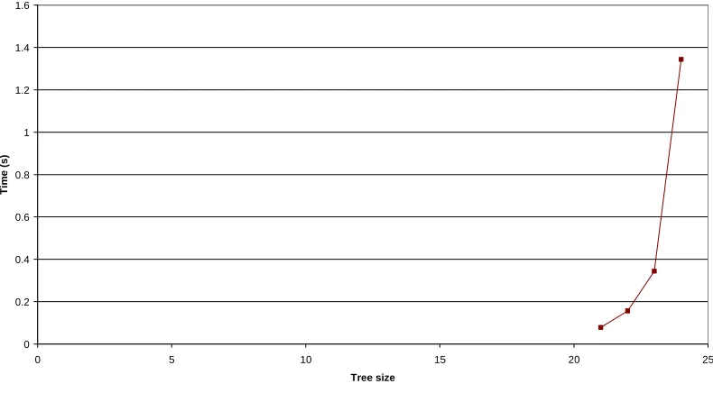
Both the mean and worst-case running time for the basic edge search increase very rapidly. Note that the worst-case time (Figure 4-10) is 5000 times worse than the average (Figure 4-11).

0 50 100 150 200 250

0 2 4 6 8 10 12 14 16

Tree size

Ti

m

e

(

s

(40)

0 0.005 0.01 0.015 0.02 0.025 0.03 0.035 0.04 0.045 0.05

0 2 4 6 8 10 12 14 16

Tree size

Ti

m

e

(

s

)

Figure 4-11: Basic edge search algorithm mean running time (arithmetic scale) These are easier to see on a logarithmic scale (Figure 4-12).

0.0001 0.001 0.01 0.1 1 10 100 1000

0 2 4 6 8 10 12 14 16

Tree size

Ti

m

e

(

s

)

Worst time (s) Seconds/tree

(41)

0 200000000 400000000 600000000 800000000 1000000000 1200000000 1400000000 1600000000

0 2 4 6 8 10 12 14 16

Tree size

C

a

ll

s

t

o

Fi

ndEdg

e

Figure 4-13: Basic edge search algorithm worst-case calls to FindEdge (arithmetic scale)

0 50000 100000 150000 200000 250000 300000 350000

0 2 4 6 8 10 12 14 16

Tree size

C

a

ll

s

t

o

Fi

ndEdg

e

(42)

1 10 100 1000 10000 100000 1000000 10000000 100000000 1000000000 10000000000

0 2 4 6 8 10 12 14 16

Tree size

C

a

ll

s

t

o

Fi

n

d

E

dge

Worst calls to FindEdge Mean calls to FindEdge

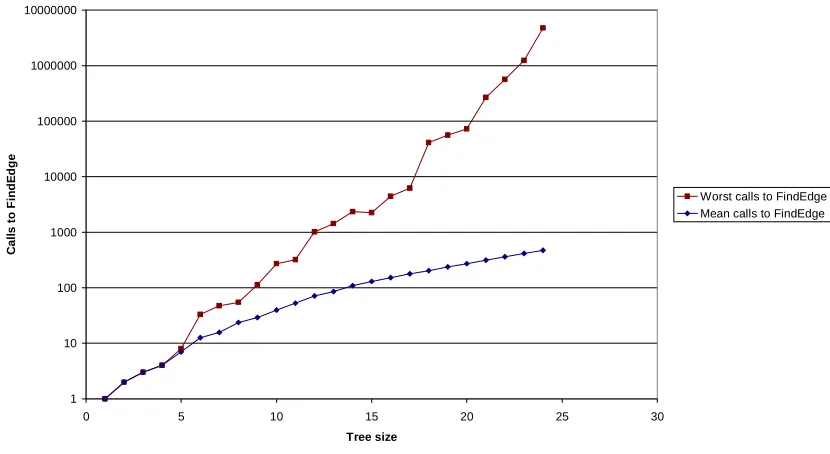
Figure 4-15: Basic edge search worst-case and mean calls to FindEdge (logarithmic scale) The basic edge search algorithm would take far too long if it tried to label most 29-node trees. However, this form was still far faster than the basic factorial-time search used in chapter 6. Several adjustments were then made to improve the running time.

4.4 Extensions

4.4.1 Restarting after excess time

The most serious problem with the edge search was its occasional tendency to get into time-consuming dead ends. For some trees, no labelling exists for certain starting nodes, yet the edge search spends a long time trying out labellings. The simplest fix was to record the time when the first node was labelled, and calculate how long the search had run. After excess time (0.2-1.0 seconds was found sufficient on the hardware used), a new starting node was chosen at random.

(43)

4.4.2 Restarting after excess failures (EdgeSearchRestart)

There were occasions when the ‘FindEdge’ procedure could not find any way to extend the partial tree. This could be recognised and counted – if the edge requested couldn’t fit anywhere, the ‘failure count’ was incremented. If the failure count exceeded a preset ‘failure tolerance’, the search was restarted with a new node. If all n starting nodes were tested and no labelling resulted, the search was restarted with two changes:

1. The adjacency list of every node was scrambled. Since nodes were added to the ‘possible’ list in their order from the adjacency list, this meant the ‘possible’ list would have a different ordering.

2. The failure tolerance was increased. This gave more chances to find a correct labelling, at the expense of more time spent searching failed labellings.

Choosing the failure tolerance starting point and increment required some adjustment. Initially, it started at 1 and was doubled after a restart.

Observation showed that a graceful labelling was often found after approximately n2 failures, so the starting tolerance was set to n2. Initially the increment was n. This worked well on the average case, but was very poor in the worst case. At size 28, one tree still suffered 2.95*107 failures after selecting the correct starting node. After observing cases like this, the increment was changed back to doubling the failure tolerance.

Failure-based restart, with failure tolerance starting at n2 and doubling after try all n starting points, worked well. It does still suffer from the same problem as the time-based restart – it is not guaranteed to terminate if a non-graceful tree exists. If the tree is graceful, the failure tolerance will eventually climb high enough that every possible labelling will be tested.

The proof of correctness in section 4.3.1 still holds, so if the algorithm does terminate, the labelling it reports will be graceful.

(44)

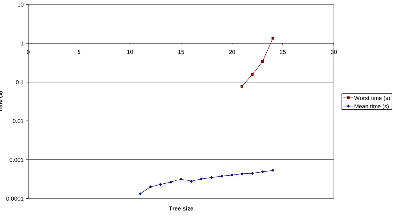
time still climbs rapidly (Figure 4-16 and Figure 4-19), but was far better in constant terms than the basic algorithm, and the mean is much shallower (Figure 4-17 and Figure 4-19). This is also apparent on the logarithmic scale (Figure 4-18 and Figure 4-21).

0 5 10 15 20 25 30 35

0 5 10 15 20 25

Tree size

Ti

me

(s)

Figure 4-16: EdgeSearchRestart worst-case running time (arithmetic scale)

0.00E+00 5.00E-05 1.00E-04 1.50E-04 2.00E-04 2.50E-04 3.00E-04 3.50E-04 4.00E-04

0 5 10 15 20 25

Tree size

Ti

m

e

(

s

)

(45)

0.00001 0.0001 0.001 0.01 0.1 1 10 100

0 5 10 15 20 25

Tree size

Ti

m

e

(

s

)

Worst time (s) Mean time (s)

Figure 4-18: EdgeSearchRestart worst-case and mean running time (logarithmic scale)

0 20000000 40000000 60000000 80000000 100000000 120000000 140000000 160000000 180000000

0 5 10 15 20 25

Tree size

Ca

lls

t

o

F

in

d

E

d

g

e

(46)

0 200 400 600 800 1000 1200 1400 1600 1800 2000

0 5 10 15 20 25

Tree size

Ca

lls

t

o

F

in

d

E

d

g

e

Figure 4-20: EdgeSearchRestart mean calls to FindEdge (arithmetic scale)

1 10 100 1000 10000 100000 1000000 10000000 100000000 1000000000

0 5 10 15 20 25

Tree size

Ca

lls

t

o

F

in

d

E

d

g

e

Figure 4-21: EdgeSearchRestart calls to FindEdge (logarithmic scale)

4.4.3 Identifying mirrored nodes (EdgeSearchRestartMirrors)

(47)

The mean running time is now very shallow (Figure 4-23), suggesting that the algorithm is very efficient for most trees. The worst-case efficiency remains exponential (Figure 4-22 and Figure 4-24), although it is very good in constant terms.

0 0.2 0.4 0.6 0.8 1 1.2 1.4 1.6

0 5 10 15 20 25

Tree size

Ti

m

e

(

s

)

Figure 4-22: EdgeSearchRestartMirrors worst-case running time (arithmetic scale)

Mean time (s)

0 0.0001 0.0002 0.0003 0.0004 0.0005 0.0006

0 5 10 15 20 25 30

Tree size

Ti

m

e

(

s

[image:47.595.136.531.131.349.2]

)

(48)

0.0001 0.001 0.01 0.1 1 10

0 5 10 15 20 25 30

Tree size

Ti

m

e

(

s

)

Worst time (s) Mean time (s)

Figure 4-24: EdgeSearchRestartMirrors worst-case and mean running time (logarithmic scale)

0 1000000 2000000 3000000 4000000 5000000 6000000

0 5 10 15 20 25 30

Tree size

C

a

ll

s

t

o

Fi

n

d

E

[image:48.595.138.536.55.274.2]

dge

(49)

0 50 100 150 200 250 300 350 400 450 500

0 5 10 15 20 25 30

[image:49.595.133.548.339.566.2]

Tree size C a ll s t o Fi n d E dge

Figure 4-26: EdgeSearchRestartMirrors mean calls to FindEdge (arithmetic scale)

1 10 100 1000 10000 100000 1000000 10000000

0 5 10 15 20 25 30

Tree size C a ll s t o Fi n d E dge

Figure 4-27: EdgeSearchRestartMirrors worst-case and mean calls to FindEdge (logarithmic scale)

(50)

0 500 1000 1500 2000 2500 3000

0 10 20 30 40 50 60 70

Tree size

W

o

rs

t-c

a

s

e

r

u

n

in

g

ti

m

e

(s

[image:50.595.139.532.74.276.2]

)

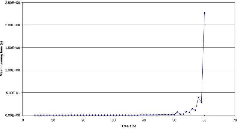
Figure 4-28: EdgeSearchRestartMirrors worst-case running time for random trees (arithmetic scale)

0.00E+00 5.00E-01 1.00E+00 1.50E+00 2.00E+00 2.50E+00

0 10 20 30 40 50 60 70

Tree size

M

e

a

n

r

u

nni

ng

t

im

e

(

s

)

[image:50.595.136.532.348.572.2]

(51)

1.00E-05 1.00E-04 1.00E-03 1.00E-02 1.00E-01 1.00E+00 1.00E+01 1.00E+02 1.00E+03 1.00E+04

0 10 20 30 40 50 60 70

Tree size

R

unni

n

g

t

im

e

(

s

)

[image:51.595.137.537.55.269.2]

Mean time (s) Worst time (s)

Figure 4-30: EdgeSearchRestartMirrors worst-case and mean running time for random trees (logarithmic scale)

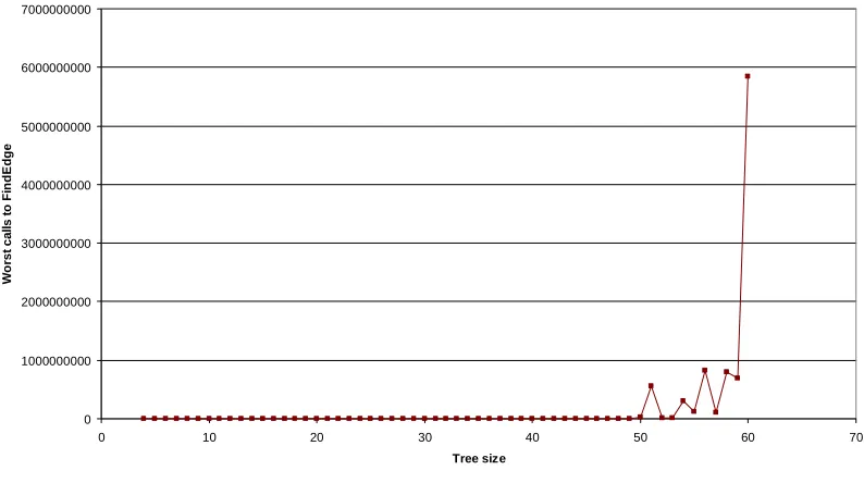
0 1000000000 2000000000 3000000000 4000000000 5000000000 6000000000 7000000000

0 10 20 30 40 50 60 70

Tree size

W

o

rs

t c

a

lls

t

o

F

in

d

E

d

g

e

[image:51.595.135.532.348.570.2]

(52)

0 1000000 2000000 3000000 4000000 5000000 6000000

0 10 20 30 40 50 60 70

[image:52.595.136.531.55.276.2]

Tree size M e a n c a lls t o F in d E d g e

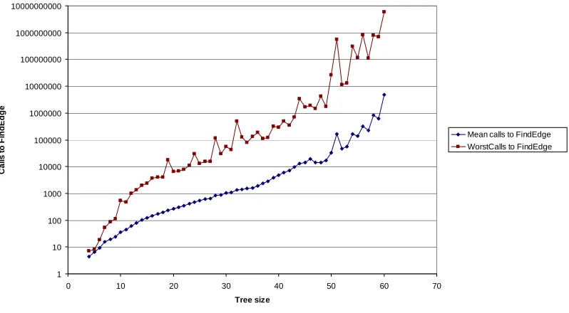
Figure 4-32: EdgeSearchRestartMirrors mean calls to FindEdge for random trees (arithmetic scale) 1 10 100 1000 10000 100000 1000000 10000000 100000000 1000000000 10000000000

0 10 20 30 40 50 60 70

Tree size C a ll s t o Fi nd E dge

Mean calls to FindEdge WorstCalls to FindEdge

Figure 4-33: EdgeSearchRestartMirrors worst-case and mean calls to FindEdge for random trees (logarithmic scale)

4.4.4 Running time comparisons

[image:52.595.137.536.348.568.2]

(53)

0.01 0.1 1 10 100 1000

0 5 10 15 20 25

Tree size

Wo

rs

t-cas

e ru

nni

ng

ti

m

e

(s

)

EdgeSearchBasic

EdgeSearchRestart

[image:53.595.136.537.57.295.2]

EdgeSearchRestartMirrors

Figure 4-34: Worst-case running time for the three forms of EdgeSearch

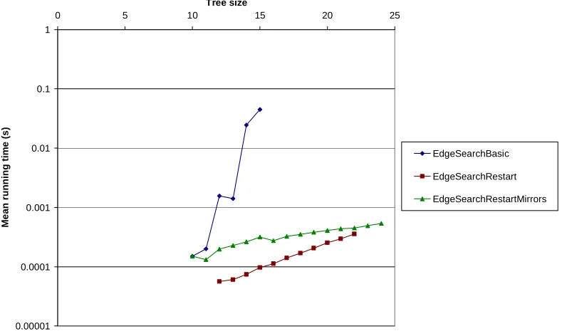
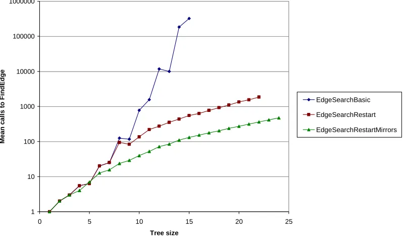
However, the average case for the EdgeSearchRestart was faster that EdgeSearchRestartMirrors (Figure 4-35) for trees with up to 22 nodes.

0.00001 0.0001 0.001 0.01 0.1 1

0 5 10 15 20 25

Tree size

M

e

an

r

u

nn

in

g

ti

m

e

(

s

)

EdgeSearchBasic

EdgeSearchRestart

EdgeSearchRestartMirrors

Figure 4-35: Mean running time for the three forms of EdgeSearch

[image:53.595.140.538.418.654.2]

(54)

1 10 100 1000 10000 100000 1000000 10000000 100000000 1000000000 10000000000

0 5 10 15 20 25

[image:54.595.135.538.57.299.2]

Tree size Wo rs t c a lls t o Fi nd Ed ge EdgeSearchBasic EdgeSearchRestart EdgeSearchRestartMirrors

Figure 4-36: Worst-case calls to FindEdge for the three forms of EdgeSearch

1 10 100 1000 10000 100000 1000000

0 5 10 15 20 25

Tree size M e a n ca ll s to F ind E d ge EdgeSearchBasic EdgeSearchRestart EdgeSearchRestartMirrors

Figure 4-37: Mean calls to FindEdge for the three forms of EdgeSearch

[image:54.595.136.537.361.602.2]

(55)

EdgeSearchRestartMirrors (Figure 4-35), suggesting that EdgeSearchRestartMirrors will be faster on average at larger tree sizes.

4.5 The edge search conjecture

The edge search algorithm does not consider every possible node labelling, due to its requirement that each edge be applied adjacent to previous edges. At every stage, the labelled edges will form a subtree. This means it could never generate the following graceful labelling in Figure 4-38, because edge label 2 is not adjacent to edge labels 3, 4 or 5.

Figure 4-38: Example of a graceful labelling not covered by the edge search conjecture

Despite this, the edge search always appears to generate a graceful labelling. This leads us to conjecture that all trees admit a graceful labelling where every edge label other than n-1 is adjacent to one edge of greater label.

This form of graceful labelling is already known; Cahit’s algorithm for labelling caterpillars will always generate a labelling of this type (Cahit & Cahit 1975). However, it has not been previously suggested that all trees admit this form of graceful labelling.

4.6 The final algorithm

This algorithm features both the changes found useful in EdgeSearchRestartMirrors. Specifically:

1. FindEdge detects when it can’t find any edge that will fit the requested edge label. This requires the new variable EdgeFound.

2. FindEdge records the number of times that it can’t find any edge that will fit. This requires the new variables FailureCount and GivenUp.

3. If the FailureCount exceeds the failure tolerance, the whole search is restarted from another node. This requires the new variable FailureTolerance. After all nodes have been tested, FailureTolerance