An Algorithm For The Selection Of A Method For
The Modelling Of Direct-On-Line Starting Of
Cage Induction Motors From Finite Supplies
by
John Michael Ameaud, BSc, MSc
in the Department of Electrical and Electronic Engineering Submitted in fulfilment of the requirements for the degree of
Doctor of Philosophy
UNIVERSITY OF TASMANIA HOBART
December, 1995
Name of Borrower Company/Department Affiliation or Contact Address
Date borrowed An Algorithm For The Selection Of A Method For The Modelling Of Direct-On-Line
Starting Of Cage Induction Motors From Finite Supplies
[Selecting An Induction Motor Model]
CKNO
\itEDGEMENTS
I would like to express sincere thanks to the following people for their help :
My supervisors : Dr Richard Langman, (University of Tasmania) for his continual encouragement and Dr Anthony Parker, (University of Adelaide) for his support in the early stages of the work.
Mr Glen Mayhew, Technical Support Manager in the Department of Electrical and Electronic Engineering who designed much of the electronic hardware used for the data acquisition so that it did what I required of it. The workshop staff of the Department of Electrical and Electronic Engineering who put Glen's designs into a useable form.
Mr Russell Twining, Computing Officer, (Network & Hardware) for his assistance with the operation of the PC systems and in particular with the transfer of textual material between different software packages.
The staff of Hobart Technical College who allowed me to have access to their Siemens motor for test purposes.
Mr John Liddell, (Neurosurgeon) and Ms Margaret Stewart, (Physiotherapist) who, each in their own way, tried to help me avoid back surgery during the final phase of the work and to the staff at the Royal Hobart Hospital who did a great job when it became unavoidable. Special thanks to Mr Guy Corkhill,
(Neurosurgeon).
Finally to my loving wife, Petula and my sons, Tim, Nick, Christopher and Simon who put up with my strange obsession for so long, with a special thank you to Christopher for the . (Unfortunately the rest of the thesis cannot live up to medieval standards of illumination).
An Algorithm For The Selection Of A Method For The Modelling Of Direct-On-Line Starting Of Cage Induction Motors From Finite Supplies
Summary
The objective of the study was the derivation of an algorithm for the selection of a numerical simulation method for the direct-on-line starting of induction motors from power supplies whose voltage and frequency may vary during the simulation period. A major part of the work consisted of an evaluation of methods for treating the variation of motor parameters under different conditions and the relative effect of these variations on predicted output. Two new methods were introduced for predicting the variation of leakage reactance with current and a new method was developed for deriving the rotor parameter variation with slip for bars of arbitrary, but known, cross-section.
An existing method was modified to derive model parameters from manufacturer's quoted performance data. The results are given of an investigation into the effect on the derived parameters and consequently on the predicted performance, of allowing the quoted performance data to vary within the tolerances permitted by Australian Standard 1359.
A set of descriptive measures for simulation output were defined. This enabled the motor's starting performance to be quantified in terms of a small number of variables. The factorial method of experimental design was used to calculate relative coefficients of performance. These related the effect of changes in program input data to the resultant variation in program output and thus allowed numerical measures to be placed on the significance of data uncertainty and model complexity as they affected the simulated performance.
PC-based data acquisition and processing techniques were used to take measurements from two laboratory motors which confirmed the results of numerical simulation work.
The broad general conclusion of the thesis was that in most situations, the total system data needs to be included in the model if the uncertainty is to be improved beyond that obtainable with simple non-recursive calculations. An expert system shell was used to present an algorithm for the selection of a method of modelling
Contents
Section Title Pg.
1. INTRODUCTION 1
1.1 Development Of The Initial Perspective On The Problem
1.2 Redefinition Of The Problem Of Formulating An Algorithm 2 1.3 Goals Of The Thesis
1.4 Exclusions From The Scope Of The Algorithm 3
1.5 Development And Use Of The Complete Simulation Model 1.5.1. Development Of The Software
1.5.2. Variation Of Circuit Parameters 4
1.5.2.1. Leakage path saturation 1.5.2.2. Skin effect in the rotor 1.5.3. Obtaining Data For The Model 1.5.4. Use Of The Simulation Model
1.6 Experimental Confirmation Of Results
1.7 The Structuring Of The Knowledge As An "Expert System" 5 1.8 The Verification Of The "Expert System"
2. CIRCUIT MODELS AND PARAMETERS 6
2.1. The Classical Equivalent Circuit 7
2.2. Discussion of Circuit Model Parameters 9
2.2.1. Stator Resistance, R1 2.2.2. Core Loss Resistor, Re
2.2.3. Magnetising Reactance, Xm 11
2.2.4. Leakage Reactance Variation With Magnetic Saturation 12 2.2.4.1. Describing function method
2.2.4.2. Logarithmic least-squares method 14
2.2.5. Rotor Resistance Variation With Leakage Path Saturation
2.2.6. Rotor Impedance Variation With Frequency 15
2.2.6.1 The double-cage circuit (DCC) model 16
2.2.6.2. The uniform deep bar (UDB) model 17
2.2.6.2.1. Depth, d, from Rgt and kir, 19
2.2.6.2.2. Depth, d', from Xdr, and Rdr.
2.2.6.2.3. Limitations of the UDB method
2.2.7. Rotor Impedance Variation With Temperature 21 2.3. Reduced Forms Of The Equivalent Circuit
2.3.1. Thevenin Equivalent Circuit
2.3.2. Other Modified Circuits 22
Section Title Pg-
2.4.1 Starting Time 22
2.4.1 Transient Torque And Current 23
2.5. Concluding Review Of Chapter 2 24
2.6. Equivalence Of Alger And Kostenko/Piotrovsky Formulae
3. PC-BASED NUMERICAL SOLUTIONS 26
3.1. A Review Of Some Commercial Packages
3.1.1 INSPEC And INSTART 27
3.1.2 CAPTOR And DAPPER 28
3.1.3 ATP4 (A Version Of The EMTP)
3.1.4 Questions To Be Asked When Selecting Commercial Software
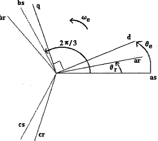
3.2. Induction Machine Free-Axis Model 29
3.2.1 General Equations And Nomenclature 30
3.2.1.1 Effect of variations in parameters 32
3.2.2 Differential Equations In Terms Of Rotor Quantities 33
3.2.2.1 Deriving the stator currents 34
3.2.2.1 Torque and acceleration
3.2.3 Differential Equations In Terms Of Flux Linkages
3.2.4 Conclusion of Section 3.2 35
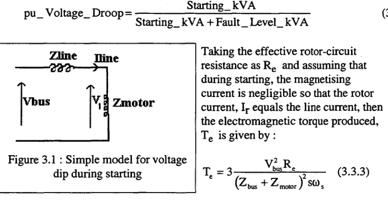
3.3 Simple Model For The Supply System 36
3.3.1 Rejection Of The Infinite Bus Model
3.3.2 Simple Approximate Models 37
3.3.2.1 Minimum generator size 3.3.2.2 Frequency droop
3.3.2.3 Other motors 38
3.3.3 Representation of AVR And Governor Action
3.3.3.1 Simple model for AVR and governor 39
3.3.4 Conclusion Of Section 3.3 40
3.4. Summary Of The Turbo-Pascal Program IM-SIM.PAS
4. FACTORIAL ANALYSIS WITH FIXED PARAMETERS 42
4.1. Description Of The Factorial Method
4.1.1 Fractional Factorial Designs 43
4.2. Application To RK4 Model Simulation 44
4.2.1 Previous Work
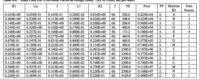
4.2.2 The Constant Parameter Study
4.2.3 Definition Of Numerical Simulation Yields 45
4.2.4 Results Of The Study 46
4.2.5 Discussion Of Results 52
Section Title Pg.
5. MODELLING PARAMETER VARIATION 55
5.1. Comparison Of Models For Leakage Path Saturation 56
5.1.1. Introduction
5.1.2. Outline Of Work Done In This Section 57
5.1.3. Existing Methods For Predicting Starting Current At Rated Voltage 58 5.1.3.1. Range of stator currents
5.1.3.2. Corrected proportional method (Cprop) 59
5.1.3.3. Logarithmic proportional method (Lprop) 60
5.1.3.4. Meilk's method (Melik)
5.1.3.5. IEE of Japan (ffiEJ)
5.1.3.6. Lee's method (Lee) 61
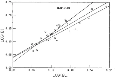
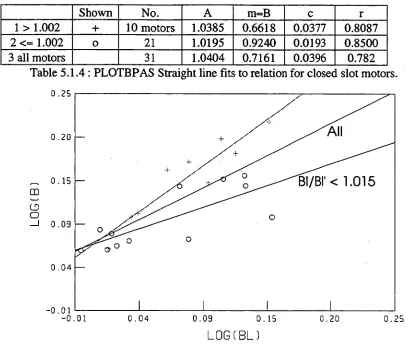
5.1.4. Some Comments On The Paper By Lee 62
5.1.4.1. Check on Lee's fits
5.1.5. New Methods For Predicting Starring Current 64
5.1.5.1. Reversed describing function method (DF1 and DF2) 5.1.5.2. Developments from Lee's method
5.1.5.2.1 For two sets of locked rotor test results (ML) 65
5.1.5.2.2 Coping with an unknown rotor slot type (UNS) 5.1.6. Method Used For Comparison Of Different Estimates Of Starting
Current
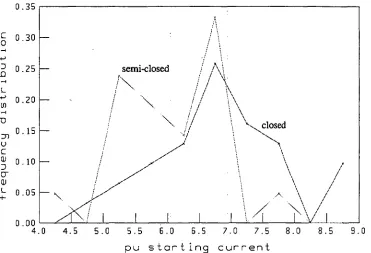
5.1.7. Calculated Errors In Predicted Starting Current 5.1.7.1. Results for closed slots
5.1.7.2. Results for semi-closed slots 67
5.1.7.3. Unknown slot type (or error in assigning type) 69
5.1.8. Choice Of Method To Limit Errors 71
5.1.9. Verification Of Original (Interpolation) Describing Function Method 73
5.1.9.1. Results of comparison 74
5.1.9.2. Complete locked-rotor saturation curve 78
5.1.10. Guidelines For Selecting A Method For Representing Leakage Path
Saturation In Simulation Programs 79
5.1.11 Programs And Files Used In Section 5.1 81
5.1.12 Verification of Error in Lee's Criteria for Semi-Closed Slots 83 5.2. Comparison Of Uniform-Deep-Bar And Double-Cage-Circuit
Models For Skin Effect In The Rotor
85
5.2.1. Double Cage Circuit Equivalent Of Uniform Deep Bar 86
5.2.1.1. Derivation of (C) from given (S }
5.2.1.2. Method used to compare derived DCC with original UDB 88
5.2.1.3. Results of deriving DCC from UDB starting point 89
5.2.1.4. Comments on the results 90
5.2.2. Uniform-Deep-Bar Equivalent Of Double-Cage Rotor 5.2.2.1 Method adopted for cage to bar comparison
5.2.2.2 Results of numerical comparison 91
5.2.2.4 Discussion of the results
5.2.3 Selection Of A Model For Skin Effect 96
5.3. The Variable-Width-Bar (VWB) Method 98
5.3.1 Derivation Of General Equation For Current Density
Section Title Pg. 5.3.3 Impedance From VWB Model 105 5.3.3.1 Checks on the computer program
5.3.4 Impedance From DCC Equivalent Of VWB Models 107
5.3.5. Comments On VWB Models 109
5.4 Simulation Of The Effect Of Temperature On Rotor Impedance 110
5.4.1 Method Used For Investigating The Effect Of Temperature
5.4.2 Results Of The Simulation 111
5.4.3 Comment On The Results 114
5.4.4 Conclusions Regarding The Effect Of Temperature 117 5.5 Magnetising Reactance And Core Loss 118
5.5.1 The No-Load Test
5.5.1.1. Method for simulating core loss
5.5.1.2. Results of simulated core loss 119 5.5.2 Rotor Core Loss
5.5.3 Magnetising Reactance Variation With Supply Voltage And Frequency
120
6. DERIVATION OF CIRCUIT PARAMETERS FROM MANUFACTURER'S PERFORMANCE DATA
121 6.1. Methods Based On Steady-State Operating Points
6.1.1 Pereira's Algorithm 122
6.1.2 Rogers And Shirmohammadi's Method 123 6.1.2.1 Efficiency Modification 124 6.1.2.2 Values at rated slip (RI , Xm and Rd) 125 6.1.2.3 Rotor resistance at starting (Rst) 126 6.1.3 The R&S Method As A Turbo-Pascal Program 127 6.1.4 Results Of Parameter Determination
6.1.5 Conclusion Of Section 6.1 129 6.2. Optimising The Matching Of The Performance Curves 130
6.2.1 Review Of Several Methods Used
6.2.2 General Comments On Previous Work 131 6.2.3 The Hybrid Method Suggested 132 6.2.4 Some Sample Cases
6.2.4.1 2.2 kW motor with single-cage rotor
6.2.4.2 7.5 kW motor with double-cage rotor 134 6.2.5 Conclusion Of Section 6.2 136 6.3. The Effect Of Manufacturer's Performance Tolerances On The
Derived Parameters
137 6.3.1 Data For Models
6.3.2 AS 1359 Tolerances
6.3.2.1 Need to restrict the tolerance range 138 6.3.3 Definition Of Yields From The Simulation Process 139
6.3.4 Results Of Simulations 140
6.3.5 Relative Effect Of Data Uncertainty And Model Sophistication 141
6.3.6 Transient Period
Section Title Pg- 6.3.8 Conclusions Regarding Effect Of Tolerances 142 6.3.9 Percentage COPs For Circuit Parameters 143 6.3.10 Percentage COPs For Dynamic Performance 144
7. OBTAINING THE CIRCUIT PARAMETERS FROM TEST
RESULTS 145
7.1. Introduction To Test Method
7.2. Methods Of Measuring Circuit Input Impedance 146
7.3. Method Used In This Work 147
7.3.1 Data Acquisition Hardware 148
7.4. Derivation of Motor Input Impedance 149
7.4.1 Unit CONVM : To Replace Comma Separator
7.4.2 Unit FOURM : To Extract Fourier Fundamental 150 7.4.2.1 Procedure PHASE_CHK : to check phase separation 151 7.4.3 Unit PPSM : To Extract PPS Components
7.5. Method Of Derivation Of Rotor Circuit Parameters From Impedance Measurements
153
7.5.1. Note On Common Approximation 155
7.6. Results Of Experimental Work 156
7.6.1. The 2.2 kW Single-Cage Motor
7.6.1.1 The "no-load" test 157
7.6.1.2 The locked-rotor test 158
7.6.1.3 Measurements at various speeds 160
7.6.1.3 Comparison of measured and simulated impedance variations 162 7.6.2 Siemens 2Ga14 Universal Experimental Machine Set 163
7.6.2.1 The locked-rotor test 164
7.6.2.2 The "no-load" test
7.6.2.3 Measurements at various speeds 165
7.6.2.4 Comparison of measured and simulated impedance variations 166
7.7 Comments On The Experimental Work 167
7.8. Calibration Of The Data Acquistion System 168
8. SIMULATION OF MOTOR PERFORMANCE 170
8.1. Some Problems Regarding Definition Of Data For The Motors Studied
8.1.1 The 8.2 MW Heat Pump Motor 171
8.1.2 The 660 kW Fumetower Fan Motor 172
8.1.3 The 373 kW (500 hp) INSPEC Motor
8.1.4 The 4 kW Siemens Double-Cage Motor 173
8.1.5 The 2.2 kW Simpson Pope Single-Cage Motor 174 8.1.6 Data for All The Motors Studied in Chapter 8 177
8.2. Comparison With Some Other Models 178
8.2.1 The Quasi-Steady-State (Equivalent Circuit) Model
8.2.1.1 Result of comparison 179
Section Title Pg. 8.2.2 Use Of Analytical Solutions For Transient Torque And Current 182 8.2.3 Space-Phasor Plots As An Extension Of The Program IM_SEVI.PAS 185 8.2.4 Errors Introduced By Ignoring Changing Inductances 186 8.3 The Effect Of Some Variations On Simulated Performance 188
8.3.1. The Load Model
8.3.2 The Finiteness of the Supply 190
8.3.3. Leakage Reactance Variation 191
8.3.4 The Effect of Winding Temperatures 195
8.3.5 Systematic Evaluation Of The Effect Of Variations 198 8.3.5.1 Definition of the variations in the factors 199 8.3.5.1.1 Inertia
8.3.5.1.2 Saturation 8.3.5.1.3 Line Impedance 8.3.5.1.4 Load Curve
8.3.5.2 Result of applying all 32 treatments
8.3.5.3 Statistical analysis of yields 202
8.3.5.4 Comments on systematic variation of factors
8.3.6 Coefficients Of Performance For Systematic Study 204
8.3.7 Data For Unsaturable Motor Models 206
8.3.8 Plan For Complete (Non-Fractional) Factorial Study 207
9. AN ALGORITHM FOR MODEL SELECTION 208
9.1. Reasons For Using An Expert System
9.2. The Structure Of The Algorithm In The Form Of An Expert System
9.2.1. Data Needed For Various Models 209
9.2.1.1. Sorting of essential and non-essential motor data 210
9.2.2. Defming The Purpose Of The Simulation 212
9.2.2.1. Purposes other than starting 213
9.2.3. Attributes Of A Model For Induction Motor Simulation
9.2.3.1. Determination of the available model for saturation 215 9.2.3.2. Determination of the available accelerating torque 216 9.3. Justification of the Algorithm
9.3.1. Case 1: 220 kW WEG Motor Starting 218
9.3.1.1. Inconsistent data 221
9.3.1.2. Incomplete data
9.3.2. Case 2: 8.2 MW Motor Starting Time 223
9.3.3. Case 3 : Supply Disturbance Problem For 1417 kW Pump Motors
Section Title Pg.
10 CONCLUDING REMARKS 228
11 APPENDIX : DOCUMENTATION OF PROGRAM IM SIM.PAS 230 A.1.1 Use Of The Default Version Of The Program
A1.2 Structure Of The Main Program Segment A1.3 The Control Data File DSU.*
A1.3.1 Diagnostics and definition of the case to be simulated A1.3.2 Various treatments which may be applied
A1.4 The Motor Data File A*.DAT
A1.5 The Program Units PART1, PART3 AND PARTS A1.6 Unit PART7.PAS : The Main RK4 Segment
12. Bibliography I
13. Index of References VIII
INDEX OF VARIABLES
Pane numbers refer to first appearance of symboL _
Symbol Description Pg.
At-. Area of core through which magnetic flux passes. 9
B Magnetic flux density 98
BR Index used for Lee's method of saturation modelling. 61
Bm Maximum value of magnetic flux density. 9
Bj Index used for Logarithmic method of saturation modelling. 60 Bj Index used for LEE of Ja • an's method of saturation modelling. 60 B 1, Index used for LEE of Japan's method of saturation modelling. 60 (C) Set of rotor parameters for DCC model of rotor. 85
CP1 pu peak transient line current 45
CP2 pu RMS line current when speed is at 0.5 pu. 140 d Equivalent depth of rotor bar derived from Rst/Rric ratio. 17
d' Value of d derived from Xrie/Rrir. ratio. 19 del_star Data in Pereira's method for motor connection type.
DF Describing function (for modelling of leakage path saturation) 12
DFR Value of DF at rated voltage 13
DF„ Value of DF at reduced voltage, ie current < Isat 13 Ef Generator excitation voltage in simple supply model. 39
Emig RMS value of induced EMF 9
f Frequency, of supply or rotor currents. 9
H Inertia constant H = 4.ko2 / (ratedVA) 176 Heen. The inertia constant (s) of the total generator capacity +
connected motor loads
37 Ii Current into stator or stator-referred per-phase equivalent
circuit
7 Referred rotor current in per-phase equivalent circuit 7
in.% Current in phase 'a' of stator 34
Ih r v Currents in blue, red and yellow phases 149
ihc Current in phase 'b' of stator '34
In Current in core loss branch of per-phase equivalent circuit 7
Current in phase 'c' of stator 14
idr current in direct axis of rotor 30
ids current in direct axis of stator 10
inr current in quadrature axis of rotor 30
inS current in quadrature axis of stator 30
Ini Current in shunt form of magnetising branch of per-phase equivalent circuit
7 Irm Starting current with reduced stator voltage., Vred 13 Isat Per-unit stator current at which locked rotor saturation curve
departs from the linear.
12
1st Per-unit stator current at starting. 19
IT1 number of positive-going zero crossings on the transient
torque/speed curve.
Symbol Description Pg.
J Current density 15
J Polar moment of inertia of motor or/and load 22
kt I Load torque representation as a polynominal function of per-unit speed, N with Thaw
terms of rated power and syncluionous speed. Tioad = Ti.. [kti + kt2(1 — N) 4 + kt3N2 ]
:
defined in 176
kt9 kt1 kt4
Kz Impedance factor (See also Appendix 1) 39
Ici Inertia factor 39
Ke Excitation factor 39
Kt Prime mover torque factor . 39
Ice Eddy current loss constant of proportionality. 9
ki, Hysteresis loss constant of proportionality. 9
Ks Ratio of unsaturable leakage reactance to total leakage
reactance, Xt0 / Xtl 237
L1 Leakage-inductance per phase of the rotor winding 30
I./2 Leakage-inductance per phase of the rotor winding 30
Lcir Self inductance of rotor phase in direct axis. 30
Lds Self inductance of stator phase in direct axis. 30
Lew Self inductance of rotor phase in quadrature axis. 30 Ling Self inductance of stator phase in quadrature axis 30
LT/1 Mutual inductance between stator and rotor phases. 30
4 Self inductance of rotor phase. 31
Ls Self inductance of stator phase. 31
30 M Peak fundamental of the mutual inductance between stator and
rotor 31
Mi Mutual inductance between stator windings 31
M2 Mutual inductance between rotor windings 31
m Double cage rotor design ratio 86
ml Value of m derived from ratio of resistance/reactance changes. 91
m9, Value of m derived from DCC model directly. 91
n Rotor/stator transformation ratio. 30
N Number of turns in a coil. 9
p Differential operator. 30
pi Rated power of motor in kW. (See Pout below) 122
Pcnre Core loss in kW. 9
Eddy curent loss in kW. 9
Pf Power factor of motor. 122
Pf1 Power factor at rated load, (as nameplate). 122
Ppm-, loss in kW 122
Ph Hysteresis loss in kW. 9
Pout Rated power output in watts. (See pl above) 237
PP Number of pole pairs in stator winding. 34
Symbol Description Pg-
R1 Stator AC resistance per phase. 7
Rotor effective AC resistance per phase referred to the stator. 7
Re
Shunt resistor representing core loss in equivalent circuit 7 Ra Resistance of rotor upper cage referred to stator. 16Rae Ac resistance of rotor. 105
rat Per-unit rating for load condition. (Used in Pereira's method). 122
Rh Resistance of lower rotor cage referred to stator. 16
Rc Shunt resistor (referred to stator) representing total core loss
per phase. 7
re Series form of Re. 152
Rnnki Cold value of resistance. . 21
Referred resistance of rotor at low slip; eg near rated speed. 15
Re Effective rotor circuit resistance per phase referred to stator 16
Value of Re at low slip. 138
11(9 Value of Re at starting. 138
Re Value of Re derived from depth d. 90
Re Value of Re derived from depth d'.. 90
Rf Value of Re at any frequency, f derived using UDB model. 16
Rhnt Hot value of resistance. 21
Rso Resistive part of input impedance at terminals at low slip 153 Rd i Resistive part of input impedance at terminals at high slip 153 Rst Referred rotor resistance at starting, slip = 1 pu 12 Rth Resistive part of Thevenin equivalent impedance. 22
{ S } Set of rotor parameters for UDB model. 85
s Induction motor per-unit slip. 7
si Per unit slip at rated condition; ie as nameplate. 22
sm Value of slip at which maximum torque, T, occurs. 22
Sm pu maximum speed 140
SP3 pu speed at which TPS occurred 140
t Time as independent variable. 23
ti time for TPM 45
t2 time for TP1 45
t3 time for TPS 45
t4 time for CP1 45
t5 time for the pu speed to settle between 0.95 and 1.05 pu 45
t6 time for current to fall below 1 pu 140
t7 time at which the last torque zero-crossing occurred 140
t8 time at which Sm occurred 140
t9 time for speed to rise to 0.5 pu. 140
Ta Torque available to accelerate motor. 34
Trnici Temperature of cold winding (See Roma). 21
Gross electromagnetic torque produced by motor. 22
Thor Temperature of hot winding (See Rhot ). 21
Tioari Load torque. 23
Symbol Description Pg. TPM Per unit peak positive transient torque, (See also pg 23) 45
TPN Per unit peak negative transient torque. 144
TPS Per unit peak torque after decay of electrical transients (pull-
out torque) as determined from model including transients. 45 Tm Per unit peak torque (pull-out torque) as determined from
steady-state equivalent circuit model. 22
Tst Per unit starting torque as nameplate or steady-state equivalent
circuit model. 18
TST Per unit starting torque as mean of TPM and TPN. 140
V1 Voltage per phase at terminals of motor or equivalent circuit 7
Vbxs Voltage applied to blue, red and yellow phases 149
Vfms Voltage at finite bus from which motor is started. 36
VII Rated line voltage of motor. 122
Vred Reduced voltage for locked rotor test for determining the
unsaturated leakage reactances. 13
Vth Thevenin equivalent voltage source behind stator impedance and magnetising branch of equivalent circuit, Figure 2.3.1.
vd, Voltage applied to direct axis winding of rotor 30
yds Voltage applied to direct axis winding of stator 30
var Voltage applied to quadrature axis winding of rotor 30 vas Voltage applied to quadrature axis winding of stator 30
w circumferential width of rotor slot. 99
w 1 Width at the top (airgap) of trapezoidal rotor slot. 100
w7 Width at the bottom (towards shaft) of rotor slot. 100
Wfw Power losses due to friction and windage. 119
x Position radially from bottom of rotor slot towards airgap 98 X1 Per phase leakage reactance of stator at specified or implied
freqency and current 7
X2 Per phase leakage reactance of rotor referred to stator under stated or implied conditions of supply voltage, frequency, slip and current
7
Xa Leakage reactance of rotor upper rotor cage referred to stator. 16
Xnh Mutual reactance between upper and lower cages. 16
Xh Leakage reactance of lower rotor cage referred to stator. 16
Xdc Referred reactance of rotor at low slip. 15
Xe Effective referred rotor circuit reactance. 16
Xe
o
Value of Xe at low slip. 138Xf%1 Value of Xe at starting. 138
Xe , Value of Xe derived from d 90
X. Value of Xe derived from d' 90
Xf Value of Xe derived from UDB model. 16
Xm
.._
Magnetising reactance referred to the stator per phase
equivalent circuit 7
_.._ Mutual reactance between phases stator/rotor referred to
stator. 7
Symbol Description Pg. X, Self reactance of rotor per phase referred to stator. 7
Xt.() Unsaturable part of rotor leakage reactance 127
Km Saturable part of rotor leakage reactance 127
Xs Self reactance of stator per phase at specified frequency. 7 Xso Reactive part of input impedance at terminals at low slip 153 Xso Unsaturable part of stator leakage reactance (See also above) 127 Xsi Reactive part of input impedance at terminals at high slip 153
Xss. Saturable part of stator leakage reactance 127 Xst Referred reactance of rotor at starting; slip = 1. 15 Xto Component of total leakage reactance which is regarded as
unsaturable, ie invariant with current. 13
Xti Total leakage reactance 13
Xti q Value of Xti derived at test voltage equal to rated voltage. 13 Xtin Value of X11 derived at reduced test voltage Vred. 13 Xts Maximum value of the component of total leakage reactance
which is regarded as saturable, ie variable with current. 13
Xth Reactive part of Thevenin equivalent impedance. 22
Xtli Unsaturated value of total leakage reactance. 13
y Distance radially from bottom of rotor slot towards airgap. 98 Ze Complex impedance of rotor at any slip, (See Xe and Re) 16 Zline Impedance in line between motor and bus, (IEEE Brown
Book) 36
Zmntnr Impedance of motor, (IEEE Brown Book method) 36
a Reciprocal of skin depth 17
ar. Value of a when cold, (See text for actual temperature) 115
ah Value of a when hot 115
Y Arbitrary constant which determines split of total leakage
reactance between stator and rotor. 7
AP The power taken from the power system by the motor during
starting (pu on generator base). 37
e Error term in calculation of starting current. 65
1, Per unit efficiency of motor 124
11 Modified efficeiency, Rogers and Shirmohammadi's method. 124
01 Angle between stator current and voltage phasors. 125
cto Magnetic flux 98
(Prir Flux linkages in rotor direct axis. 33
(Nis Flux linkages in stator direct axis. 33
(Pnr Flux linkages in rotor quadrature axis. 33
(Pris Flux linkages in stator quadrature axis. 33
p Resistivity of material used in rotor conductor or laminations. 9
co Angular frequency of supply 31
(14 Angular velocity of freely rotating reference frame. 30
cori Angular velocity of rotor in electrical radian per second. 30 wr Actual angular velocity of motor shaft (mechanical radian per
second).
1. INTRODUCTION AND OVERVIEW
1.1. Development Of The Initial Perspective On The Problem
The work which is the subject of this thesis took place between 1987 and 1995 but the motivation for selecting the topic arose from much earlier experiences whilst I was a design engineer at GEC Large Machines at Rugby in England. At that time I was faced with the problem of determining the voltage dip experienced in offshore power systems due to the starting of large pump motors. I was aware of the difficulty of predicting accurately the sub transient and transient reactances of the solid-pole synchronous machines. The computational models available at that time did not always give results which compared well with those obtained from sudden short circuit tests. I began to wonder if the induction motor loads were subject to the same inaccuracies and inconsistencies and if the advantages gained by using a sophisticated simulation method were outweighed by the additional data that such methods seemed to require.
Whilst at the Whyalla campus of the (then) South Australian Institute of Technology, I began to look seriously at the use of numerical simulation of induction motor performance. At that stage I developed a model for the induction motor based on differential equations in fixed axes. This was an early version of the program IM_SIM.PAS, the current version of which is documented in Chapter 3. The manufacturer's quoted motor equivalent circuit parameters were used as a starting point with the simulation yielding graphs of current and torque. The values of the equivalent circuit parameters were held constant during the simulation. I became concerned with the extent to which predicted performance was dependent on small changes in the input data. For example, variation in the actual supply voltage or frequency from the nominal value would contribute to a difference between the simulated performance and that of the actual motor. This may seem obvious but most published simulation work seemed to proceed on the basis that all the required input data was available with zero uncertainty. This will be discussed further in Chapters 6 and 8.
The factorial method of experimental design was used to establish relative coefficients of performance which related the effect of changes in program input data to the resultant variation in simulated motor performance (program output). This allowed a numerical measure to be placed on the significance of the uncertainty in each program input data item as it affected the predicted output; eg the effect of leakage reactance on peak transient torque. This work is reported on in Chapter 4. As a result of this study it was concluded that for constant parameter models, the most significant data items were supply system voltage and frequency. This means that an assessment of the proposed model prior to simulation should include an estimate of the degree of finiteness of the supply bus. It also became clear that where the equivalent circuit parameters do vary during the simulation, this variation needs to be modelled fairly accurately. This point was reinforced by some useful discussions with Dr Cohn Grantham (of the University of New South Wales) on the subject of motor modelling and parameters.
found that manufacturer's quoted motor parameters are sometimes based on rated load conditions and consequently may not give realistic results when used in models designed to calculate starting or pull-out conditions. This led to a re-appraisal of the project's objectives.
1.2. Redefinition Of The Problem Of Formulating An Algorithm
The problem was redefined in terms of using the performance parameters as a starting point and adopting inverse modelling techniques to derive a set of parameters for a specified equivalent circuit, such that the error over the known performance range was minimised. The simulation exercise was then seen as an extrapolation in the performance space defined by the set of terminal vector quantities {voltage, current, speed and torque). The problem was examined from the point of view of a project consulting engineer rather than that of a motor designer. Consequently, it was assumed that the motor itself was not available to the algorithm user. Data for the numerical model could only be obtained from either type tests or from manufacturer's quoted performance data, ie access to design data was precluded.
The determination of a pathway from the performance data to the induction motor circuit model had largely been performed by Rogers and Shirmohammadi, [1987]. The method was available as a commercial computer program, [Rogers, 1993] but this often gave a close fit only to the starting and pull-out conditions and was prone to fail completely with small motors. Substantial email/fax discussions ensued between the author and Mr. Rogers which led to a revised version of the software being produced in mid-1995. In the interim, the program PARAM.PAS was developed by the author and this is discussed in Chapter 6.
The relative performance of different models was of primary concern in the formulation of the algorithm. It was recognised that a review of available models would have to be conducted. It was noted at an early stage that many sophisticated computer models existed, that all of these were claimed to work, that in general, there was little cross-referencing between published work and almost no comparison of different models using the same data. The issue of data uncertainty due to the
reluctance of manufacturers to reveal design information or to include wide tolerances in performance data (as permitted by AS 1359) was recognised. The objective of the study was then formulated.
1.3. Goals Of The Thesis
The goal of the project was stated to be the development of an algorithm for the selection of a suitable method for the simulation of the dynamic performance of the induction motor under direct-on-line starting conditions taking into account the uncertainty created in simulation output by data un-availability or uncertainty. This required :
• The development of a thorough understanding of the detailed models for modelling motor parameter variation; described in Chapter 5.
• An appreciation of the relative significance of the effect of finite power systems on supply voltage and frequency; demonstrated in the simulation work of Chapters 4 and 8.
• An assessment of the relative importance of all the various simulation program input data items; developed as a result of the simulation work of Chapter 8.
• An appreciation of the effect of being forced to use a simpler model due to lack of motor or system data; Chapter 8.
1.4. Exclusions From The Scope Of The Algorithm
The parameters derived were to be used in models of the induction motor operating from sinusoidal, balanced 3-phase mains operating close to rated frequency. The motor parameters were required to be valid over the slip range from starting to rated slip and over the operating current range from the rated-voltage starting current down to below rated current. The modelling of the performance of power electronic variable speed drives (VSDs) is excluded from the study. However, if the harmonic content of the drive may be ignored, then little error may result from the use of parameters derived using the algorithm described, provided that the action of drive feedback-control modules is incorporated into the simulation model.
The simulation of bus transfer, cyclic load shedding or the effect of transient
disturbances to the supply, other than those- caused by the motor itself, were not the prime focus of the study. The algorithm was initially designed to give guidance to the selection of a model for direct-on-line starting only. In the course of the literature survey additional knowledge was accumulated pertaining to problems other than simple starting. This arose naturally from the consideration of the effect on motors already running, of starting the motor which is the prime subject of the simulation. For these other motors, the starting of the new motor appears as a transient supply
disturbance. The bus transfer problem may be regarded as an extreme form of the supply disturbance situation. Many of the guiding principles were found to be common to all types of numerical simulation work with induction motors. The algorithm was formulated in terms of an Expert System which was extended to include some advice regarding the simulation of problems other than starting. Formal validation of the Expert System was restricted to the case of direct-on-line starting only.
1.5. Development And Use Of The Complete Simulation Model
Although the presentation given here is sequential, the actual work described in the thesis proceeded in an iterative manner. As various elements were investigated they were incorporated into earlier developments. The path to achieving the objectives of the thesis was somewhat tortuous and the subjects inter-related so that at times it became difficult to see the overall picture because of the detail. As a result it was decided in the writing of the thesis to give the reader an early overview of the work done that is somewhat longer than that allowed in a formal synopsis.
1.5.1. Development Of The Software
Generally, commercial software does not allow modification of the computational algorithms within the simulation process in order to include or exclude certain effects or compare different methods of modelling. Because of this, the program,
significant, differences between the method suggested by Rogers and Shirmohammadi in the paper referred to earlier and the commercial program.
By writing my own software I was able to incorporate the Turbo-Pascal procedures, which were used within the Runge-Kutta method for parameter variation, into a similar program based on the steady-state equivalent circuit. This guaranteed that any differences were due to the motor equations rather than to different treatments of parametric variation. Chapter 3 discusses the programs in detail and gives instructions for using default versions which produce graphs and text files for the simulated
response for six selected motors.
1.5.2. Variation Of Circuit Parameters
A major part of the work consisted of an evaluation of methods for treating the variation of motor parameters under different conditions and the relative effect of these variations on predicted output.
1.5.2.1. Leakage path saturation
The variation of stator and rotor leakage reactances due to leakage path saturation was investigated. Statistical analysis was performed of the errors introduced by using several different methods for predicting the variation of leakage reactance with current. Two new methods were introduced which have the advantage of requiring less data than the established best method whilst retaining reasonable accuracy.
1.5.2.2. Skin effect in the rotor
The uniform-deep-bar (UDB) and double-cage-circuit (DCC) methods used for modelling rotor parameter variation due to skin effect were compared. Both models are based on the values of the referred rotor reactance and resistance at zero and unity slip. It was shown that given the parameters of the UDB model, an exact equivalent DCC model can be derived but not always conversely. For some double cage rotors, the derived UDB model, gave the correct rotor impedance at zero and unity slip but was grossly in error for slip values in-between. The analysis of the uniform bar was extended to develop a new method for deriving the rotor parameter variation with slip for bars of arbitrary, but known, cross-section.
1.5.3. Obtaining Data For The Model
Various methods for obtaining the equivalent circuit parameters were assessed. The method finally adopted is discussed and justified in Chapter 6. It is emphasised that the circuit parameters as quoted by manufacturers are not to be trusted to give a reliable prediction of performance over the complete operating range of the motor.
L5.4. Use Of The Simidation Model
Simulated performance was compared using models with a range of complexity and the relative effects of model complexity and data uncertainty were assessed. This work is presented in Chapter 8 which includes a systematic study of the effect of varying some of these features.
1.6. Experimental Confirmation Of Results
Two small laboratory machines were used to verify the results of simulation work. One of these motors had a single-cage rotor and the other was of the double-cage rotor type. The test data was recorded by a new test procedure based on fast data acquisition using a PC. This work is discussed in Chapter 7.
Later a comparison was made between the set of parameters obtained from tests and those derived from the performance specification. The comparison between the two sets of performance data for each motor; one based on test results and the other derived from quoted performance data is considered to be more significant. These results are given in Chapter 8. It was recognised that tests on a larger range of motors would be desirable so such data was willingly utilised whenever available.
Advantage was taken of the availability of locked-rotor test results performed by the TEE of Japan, [1980] for 52 motors. Some starting information for a 660 kW motor was supplied by Comalco Aluminium (Bell Bay). Comparisons were also made between simulation results using the author's simulation program and simulation/test results published by Rogers and Shirmohammadi for a 8.2 MW motor, [1987].
1.7. The Structuring Of The Knowledge As An "Expert System"
The goal of the work described in this thesis has always been to present the experience gained in the form of an algorithm : a structured set of rules for attaining an objective. The use of an Expert System shell was not considered in the early stages. Since most of the simulation and experimental work involved numerical programming it seemed initially that the algorithm would take the form of a program, probably written in the Turbo Pascal language, which would evaluate the available data in terms of the simulation objectives. This was finally rejected in favour of an Expert System, mainly because this allowed forward and backward chaining through a rule set which could be added to as knowledge increased. The expert system also allowed easy communication to the user; for example, of the implications of lack of requested data.
One of the main advantages of the choice to use an expert system was that it forced the codification of the information which required the development of a deeper understanding of the relationship between the system variables. This process is summarised in Chapter 9.
1.8. The Verification Of The Expert System
The documentation of the verification of the expert system is based on four test cases. This represents a small subset of the many test runs that were performed using the software. The comments and predictions of the algorithm were assessed in the light of the experience reported in the earlier chapters of the thesis. Where errors of 'judgement" were made by the algorithm during the verification process, the program was stopped and the reason for the false conclusion identified and rectified. Notes were made regarding helpful comments or references so that these could be added to the algorithm to be brought to the attention of the user.
2. CIRCUIT MODELS AND PARAMETERS
This chapter includes a review of the standard and some less well known circuit models of the induction motor so that material found in disparate undergraduate texts and some quite old publications would be brought together in one place. Whilst I had some reservations about this, I recognised that most of the material would be
unfamiliar to many readers since it is not introduced into current undergraduate courses and is unfashionable at postgraduate level. The chapter therefore serves as a critical review of the approximations, assumptions and methods used in induction motor modelling. By including such a review I hoped to assist those beginning work in the area of induction machine modelling.
An appreciation of the relative importance of the various motor parameters under different circumstances and the ways in which they vary during machine operation was developed by the author gradually over the whole period of the study and in some ways this paralleled the historical development of induction motor modelling. For example, the first application (described in Chapter 4) of the Runge-Kutta method to solve the differential equation model, was based on a constant circuit parameter model. This led to the detailed investigation into parameter variation described in Chapter 5 and the use of performance rather than circuit parameters as the starting point for the simulation processes, (Chapter 6). These three chapters form an essential background to the developments introduced in later chapters
In this work, the focus is on models which use a limited amount of design data since, in the experience of the author, complete data is often unwillingly given by
manufacturers and when supplied, may include estimates or large unspecified tolerances. This situation precluded the use of hybrid circuits, [GO1, 1986]; finite element models for the determination of reactance, [Belmans et al, 1990], or core loss, [Zhu and Ramsden, 1993] and the use of detailed design information such as the dimensions of radial ventilation slots, [Williamson and Flack, 1994]. This restriction meant that when leakage path saturation was considered in Chapter 5, an empirical method was used because the design approach could not be adopted, [Agarwal and Alger, 1960].
The commonly used equivalent circuit model is expected to represent the machine. To do this, the circuit and machine must have the same appearance to an observer
throughout the operating range. This means that the stator voltage and current, shaft torque and speed must be the same, and consequently, so will power factor and total losses. There are three operating conditions which are usually of interest namely; starting, near rated load and run-up from rest to close to the no-load speed. Test data will not normally be available for the whole region of interest. If it were, then there would be little point in doing the simulation. The main purpose of numerical
the modelling process. The challenge is to obtain information about the machine's performance over as wide a range of operating conditions as possible with a small amount of readily available data.
In order to determine the equivalent circuit parameters, measurements are usually taken at slip values of 1 and close to zero giving Locked-Rotor (LR) and No-Load (NL) test results respectively, [IEEE, 1988]. These tests yield two complex
impedances. The stator resistance is measured separately. The circuit model which is derived from these tests is not the machine. This statement may sound trite but failure to appreciate it is the source of much error. In particular, it will be shown in Chapters 5 and 8 that it is dangerous to assign reactance values to the machine when these are properties of a particular circuit used as a model. In other words, a value for a circuit parameter cannot be quoted unless the form of the circuit is specified. There are several possible circuits which may adequately model a given machine in the steady state. In the absence of a circuit specification, the only impedance which may be assigned to the machine with complete lack of ambiguity is that derived from the voltage/current relationship at its terminals. All the others are dependent on
conceptual models which the observer brings to the test results and assigns parameter values in order to conform with the behaviour measured at the machine's terminals.
2.1. The Classical Equivalent Circuit
The classical equivalent circuit of Figure 2.1.1 has 6 parameters. The standard test data obtained as above yields five real numbers. The circuit therefore contains one degree of freedom so that, in practice, several versions of the steady-state equivalent circuit exist, all of which will match the given test data. In particular, in the absence of design data it is impossible to separate the stator and rotor components of leakage reactance with any degree of accuracy from measurements made at the motor
terminals, [Jones, 1967] and [Grantham, 1985].
Figure 2.1.1: Classical "exact "equivalent circuit
With many small machines, where the variation in rotor parameters with slip may be ignored, it is unnecessary to separate the leakage reactances. Jones showed that the equivalent circuit may be represented (in terms of self and mutual reactances,
Figure 2.1.2: General form of the equivalent circuit in terms of self and mutual reactances
Figure 2.1.3 : Equivalent circuit of Figure 2.1.2 with y = Xs / 3C-n,
In cases where the rotor reactance is known to vary with the frequency of the currents induced in the rotor, it becomes conceptually difficult to combine the stator and rotor reactances into a total leakage reactance. The question then arises of how to divide the total reactance into its frequency-sensitive and frequency-insensitive parts. Simulated machine performance is then highly dependent on the allocation of total leakage reactance between the rotor (taken as variable with slip) and stator (taken as invariant with slip).
Three of the circuit parameters (R1 , Xm and Re) are shown in Chapter 4 to have relatively little influence on the predicted dynamic performance of the motor during direct-on-line starting. This agrees with the work of Smith and Hamil mentioned previously. It is interesting, however, to examine the effect of errors in R1 on the derived value for Rc. If a slightly smaller value of R1 were used in the analysis of the locked-rotor test results then the effect would be to produce a slightly larger value for the referred rotor resistance, R2 and to marginally affect the value deduced for Rc
2.2. Discussion of Circuit Model Parameters
2.2.1. Stator Resistance, R1
Strictly, the value used should be the ac resistance which allows for skin effect in the stator conductors. Unlike the rotor, these are usually stranded. This is done partly in order to minimise the deep-bar effect. This effect is usually allowed for by multiplying the measured dc resistance by a factor of approximately 1.1 to derive the ac
resistance, [Gosbell and Dalton, 1991]. The dc resistance is commonly measured directly using one of four methods.
1) Direct measurement using a hand-held multimeter 2) The Ware test, [Bourne, 1969]
3) As the slope of a curve of dc supply voltage against current 4) Using a four-terminal bridge circuit.
The last two methods seem preferable but as mentioned, the accuracy is not critical. In any case, it would be pointless to measure the dc resistance accurately and then multiply it by a factor whose value could lie between 1.05 and 1.15.
The effect of errors in the assigned value of R1 is to change the value of referred rotor
resistance, R2 derived from locked-rotor test results. The most sensitive indicator of the low-slip value of rotor resistance is the slip at which maximum electrical torque occurs (See Section 9.2.3). This is difficult to measure with any accuracy.
2.2.2. Core Loss Resistor,
Hysteresis loss is usually modelled by Ph = khffimx (2.2.1) where Bm is maximum flux density and 0.8 x 2.3.
(usually close to 2 for modern core material).
Similarly, the eddy current loss is given by Pe = [ket2 f2Bm2]1 p (2.2.2)
The induced EMF, E rms = VafNAcil„, (2.2.3)
If the ratio of Erms to frequency, f is kept constant, then the flux density will be
constant. This condition will be approximately satisfied if the power system is such that the frequency and voltage do not change much, (ie. an infinite-bus system). Core loss is then given as 'core = Ph ± Pe kl 7 12 (2.2.4)
Here k represents some constant of proportionality and the applied voltage and induced back EMF are taken as approximately equal. This is reasonable if, as is usual in practical motors and transformers, the voltage drop due to leakage reactance is small. This loss can then be represented by a constant resistance in parallel with the magnetising reactance.
Measurements with an Epstein frame in the rage of 50 to 2000 Hz over a temperature range of 20 to 220 0C have suggested that the core loss is proportional to the cube of the flux density, [Mouillet et al, 1994] but this has not been supported by
with accurate measurement of core loss under dynamic conditions and the uncertainty in total losses.
In practice, other (stray) machine losses are also present and the uncertainty due to these is usually combined with the core loss uncertainty to result in an overall uncertainty in energy flow within the motor. The author's experience is that the measured frictional torque may vary between motors of the same nominal design due to manufacturing inconsistencies. These uncertainties add to those which might arise from inadequacies in system modelling, particularly if variable voltage or frequency conditions are encountered. For example, in marine systems, where frequency dips of 5% may be combined with voltage dips of 25% during the starting of large motors. These factors may lead to inaccuracy in the prediction of net shaft torque. This sets limits on the degree of precision that should be sought in modelling the "constant losses".
For a given motor, the friction and windage (F&W) loss is constant at constant operating speed. For induction motors at fixed frequency, the speed is approximately constant over the normal operating range. During starting, the F&W loss is reduced at lower speeds but there are additional core losses in the rotor due to the fact that the rotor flux during starting is at a higher frequency than under rated load operation. In practice the extra rotor core loss compensates for the reduced F&W loss and the assumption of constant core loss remains valid to a reasonable degree of
approximation. For VSD modelling this method breaks down as low rotor frequency and reduced rotational friction losses can co-exist. However, the overall loss may well be of a similar order since the harmonic losses will be greater (but not precisely known) due to the non-sinusoidal VSD supply.
Another approach to core loss modelling is to recognise that the loss is associated with the total stator flux linkage (leakage as well as mutual flux) and to place the resistor used to represent core loss as in Figure 2.2.1, [Andria, Dell'Aquila, Salvatore and Savino, 1987]. In theory this seems reasonable but it assumes that accurate allocation of stator leakage can be done. From a circuit point of view it is possible to derive a combination of parameter values for Figure 2.2.1 which has the same input impedance at a given slip as Figure 2.1.1
Figure 2.2.1 : Non-conventional core loss representation
Rogers and Shirmohanunadi, [1987] ignored core loss altogether and compensated for it by increasing the mechanical losses. This results in adjustments being made to the other circuit parameters in order to match the required power factor.
overcome mechanical no-load losses so that a small amount of power is used in the rotor circuit. The effect of assuming that the input impedance on no-load is given by the circuit of Figure 2.1.1 with slip set equal to zero, is discussed in Chapter 5.
It seems more precise to represent the mechanical losses by a speed dependent loss, to make Rc variable with frequency and flux level and to measure core losses with the machine driven at synchronous speed. In practice, if data which would allow the accurate separation and modelling of friction and windage losses over the region of interest is not available, then it seems inappropriate to be overly concerned about the accurate representation of core loss.
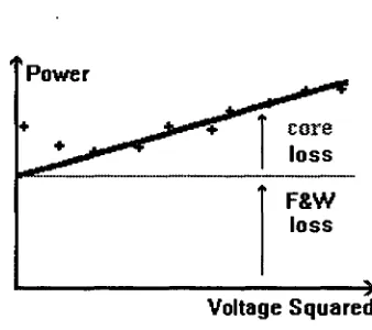
Usual practice is to separate the
friction and windage loss from the core loss by performing the NL test over a range of stator voltages [IEEE, 1988, Section 5.6.2]. The input power (less stator copper loss) is plotted against voltage squared as shown in Figure 2.2.2. At low voltages, the slip rises and the results are ignored. A straight line extrapolated back to the power axis has an intercept equal to the friction and windage loss ie. the input power (less stator copper loss) with core loss reduced to zero.
[image:28.577.315.484.221.371.2]Voltage Squared
Figure 2.2.2 - Loss separation
2 2.3. Mavetising,Reactance, Xm
Magnetising current is dependent on flux level, so it seems reasonable that the value of Xm selected for inclusion in a model is based on tests done at an appropriate level
of main-flux ie at the same level as would occur under the condition to be simulated, [de Mello and Walsh, 1961]. With infinite-bus mains supplies, this means at rated voltage less the voltage drop in the stator. In the simulation of induction motor
starting, the voltage dip may be up to 25% in mining or offshore systems and the level of the dip is unknown until the simulation is done. Under these conditions, the motor magnetising reactance may vary from the normal (slightly saturated) condition to the unsaturated (as the voltage dips) then to a condition of greater than usual saturation (as the frequency falls and the automatic voltage regulator increases excitation) and then back to normal saturation as the frequency returns to normal (the governor regains control). The level of magnetising path saturation may also vary from the• nominal design condition if a motor designed for use at one voltage level is in fact used on a system of a slightly different voltage. This situation is likely to occur more often with moves to broaden permitted tolerances on supply voltages; eg. 415/240V or 380/220V motors operating on 400/230V supplies.
Saturation along the main flux path has been shown to have little influence on the starting condition, [Sivokobylenko and Kostenko, 1980]. The usual practice is to determine Xm from the NL test. Like 12c ,the effect of assuming that the NL slip is
zero is to generate an inaccurate value for Xm. However since, as will be shown in
Chapter 4, the predicted motor dynamic performance during starting is relatively insensitive to variation in Xm , the NL test results may be used in such studies without
Stability at an operating point may be significantly affected by saturation in the main flux path, especially where the system has a limited amount of natural damping, [He and Lipo, 1984]. This means that the modelling of the effect of transient voltage disturbances on a lightly loaded motor may need to allow for the effect of main flux saturation on Xm (and on the leakage inductances due to the self-inductances being under saturated conditions).
2.24. Leakage Reactance Variation With Magnetic Saturation
The total referred leakage reactance is the most important machine parameter in that the predicted performance is highly dependent on it, (See Chapter 4). The total leakage reactance decreases with increased current due to saturation of leakage flux paths. For some machines with complex slot shapes this can occur at relatively low currents due to a deliberate attempt by designers to improve starting torque/ampere. This is especially true of smaller machines with cast aluminium rotors and can make the prediction of full-voltage starting current difficult. Considerable work has been done to allow starting currents to be predicted based on the results of up to three reduced-voltage locked rotor tests, [Lee, 1989]. Two methods are introduced here with a detailed comparison being left until Chapter 5.
It is noted that since the measurement of LR voltages and currents takes place during steady-state tests after the decay of the electrical transients, these methods give the steady-state reactance. The starting currents derived from them will not include
transient dc offsets which may need to be taken into account when setting overcurrent protection relays. This is confirmed in Chapter 8.
2.2.4.1. Describing function method
One approach that is sometimes used to model leakage path saturation is the describing function. A variant of this is given by Chalmers and Mulki, [1970]. The method outlined here is that of Rogers and Skirmoharnmadi, [1987] which is similar to that used in the lNSPEC/INSTART package discussed in Chapter 3. The notation agrees with that work. Define a describing function parameter, DF such that
for any stator current, RIsat, DF = 1 2
and for I>Isat, DF = [ + — si n (2)1 2 1
(2.2.5)
where = sin -1 i/sat
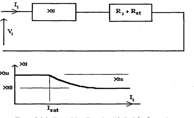
At starting, we can neglect the magnetising branch so the total leakage reactance, X ti
2
is given by, x1 =11(-1d — (R1 + R, )2
Xt I R + Rst
TV,
Xt s
[image:30.574.136.470.54.257.2]sat
Figure 2.2.3 : Describing Function Method for Saturation
Two data points are needed from locked rotor tests, one at full voltage and the other at reduced voltage, Vred as shown in Table 2.2. These allow saturated (subscript, s) and unsaturated (subscript, u) values of the total leakage reactance, Xtl and describing function, DF to be calculated.
Test Voltage, V1 Vi = lpu Vred
Test Current, II 1st Ired
Derived Reactance, Xtl Xtls Xtlu
DF DFs DFu
Table 2.2: Data needed for describing function method
Since Xtlu and Xtls are given by
Xtlu = Xt0 + DFu Xts and Xtls = Xt0 + DFs Xts
the saturated and unsaturated parts of the total leakage reactance as shown in Figure 2.2.3 may be separated as :
Xts = (Xtlu-Xtls)/ (DFu-DFs) and Xt0 = (Xtls DFu - Xtlu DFs)/(DFu -DFs)
The leakage reactance, Xtl at any current, I can then be determined by using an appropriate value of DF derived from equation (2.2.5) and from
Xtl = Xt0 + DF Xts (2.2.7)
For this method it is assumed that the onset of saturation occurs at a particular value of stator current, Isat. The describing function method is compared with other methods in Chapter 5 and with experimental results in Chapter 7.
A similar describing function was used by Smith, Rogers and Buckley, [1979] but in this case allowance was made for the fact that saturation affects the different
2.2.4.2. Logarithmic least-squares method
This method and the example given are taken from Melik, [1987].
Let the RMS starting current, I at any RMS line voltage, V be given by I = A VB
Hence ln(I) = ln(A) + B ln(V) {where ln(x) is natural log of x)
Writing In(A)=a gives In(I) = a + B ln(V) to which a least-squares fit yields constants A and B. e.g. for
I 67 87 168 V 1752 2170 3640
we get A=0.005468 and B=1.26.
At rated voltage of 6600 V. the predicted starting current is then 355 A (The actual test starting current given in the paper by Melik was 357 A)
Assuming a star circuit model, the total input impedance per phase at starting is given V
by Z = . Since the magnetising current is usually much less than the starting
-4 31
current the magnetising branch may be neglected to give the total leakage reactance as
Xd
--
-1(
1
81 2
— (RI ± R2) (2.2.8)
-13
-
0
Melik's method is the logarithmic proportional method with the curve-fit constants determined as a least-squares fit based on three data points. The direct proportional method is a special case of the logarithmic proportional method where B=1 and A=Ired/Vred.
In Chapter 5, two other modified forms of the logarithmic method in which the values of constants A and B are assigned based on statistical analysis of 52 tested motors are discussed and two new methods are introduced. All four of these methods are shown to be improvements on the logarithmic least-squares method described above.
2.2.5. Rotor Resistance Variation With Leak a • '• . •