Extending and Benchmarking Cascade-Correlation
Extensions to the Cascade-Correlation architecture and
benchmarking of feed-forward supervised artificial neural
networks
by
Samuel George Waugh, BSc (Hons)
Submitted in fulfilment of the requirements for the degree of Doctor of Philosophy
%06.1,11
.
a'
IONA
Tkitu4
Li) AUG-H
P
Abstract
This thesis is divided into two parts: the first examines various extensions to Cascade-Correlation, and the second examines the benchmarking of feed-forward supervised artificial neural networks, including back-propagation and Cascade-Correlation.
The first extensions to the training mechanism of Cascade-Correlation involve the inclusion of patience to stop the addition of hidden nodes and the introduction of alternative methods for training the candidate pool. These methods greatly improve the training speed of the algorithm. Secondly, reducing the number of connections within Cascade-Correlation networks is examined: by the introduction of hidden nodes with limited connection strategies, and by the pruning of the fully-connected hidden nodes and the output layer. Three methods of stopping the pruning process are briefly investigated. It is shown that adding limited connected hidden nodes is effective in altering the style of network topology, if not reducing the number of connections. Pruning within Cascade-Correlation drastically reduces the number of connections required without affecting the classification performance of the networks developed. Furthermore, all the different methods of halting the pruning process are shown to be effective.
The second part of the thesis concentrates on benchmarking feed-forward supervised artificial neural networks, in particular Cascade-Correlation. The earlier part of the thesis highlights the need for effective benchmarks, as a large number of real-world problems do not require anything more than a single layer of weights to achieve near optimal
performance given the available data. The second part initially investigates two new real-world problems. Although both turn out to be useful problems to examine — testing many of the features of Cascade-Correlation described earlier — they too do not require much more than a single layer of weights, and hence do not test the power of Cascade-Correlation or other systems which allow the use of hidden nodes. Two methods of generating artificial data are then examined as ways of producing increasingly complex data sets. The
Statements of originality and access
This thesis contains no material which has been accepted for a degree or diploma by the University or any other institution, except by way of background information and duly acknowledged in the thesis, and to the best of my knowledge and belief no material previously published or written by another person except where due acknowledgment is made in the text of the thesis.
...eara•P••—...-- _i,._,,j-
This thesis may be made available for loan and limited copying in accordance with the Copyright Act 1968.
Acknowledgments
Thanks to my supervisors Tony Adams and Phil Collier: their help and insightful comments were invaluable. Thanks particularly to Tony, who cheerfully put up with me annoying him every week. Thanks also to Scott Fahlman who was of great assistance during the initial development of this work, and who is always ready to answer questions. Further thanks to the anonymous examiners for their helpful comments and suggestions.
Thanks also to the members of the Artificial Neural Network Research Group and the department's postgraduate students — particularly Julian Dermoudy, Carl Lewis, Peter Vamplew, Tim Freeman and Lee Arnould — who helped my postgraduate studies go a little faster.
Acknowledgment and thanks must also go to other groups for their assistance in producing this thesis. Thanks to the Tasmanian State Government Department of Education and the Arts for providing after-hours access to their machines, resulting in over 13000 hours of simulations being completed. In particular, Jim Palfreymann and Dr John Gilbert deserve special mention. To the Tasmanian Government Department of Primary Industry and Fisheries Marine Research Laboratories, in particular Warwick Nash, for generously providing the abalone data. To the University of Newcastle Centre for Linguistic and Literary Studies, in particular John Burrows and Hugh Craig, for the data on Romantic and Renaissance tragedies. Finally thanks to Michael Fraser, Simon Talbot and Tony Adams, respectively, for suggesting these resources in the first place.
The patience and assistance of the many proof readers who made it through the earlier drafts also deserves recognition, in particular Tony Adams, Trudy Steedman, Cristina Cifuentes, Phil Collier and Julian Dermoudy.
Contents
Abstract i
Statements of originality and access
Acknowledgments iii
1 Introduction 1
1.1 Organisation of thesis 2
1.2 Inclusion of papers 3
Part I Extensions to Cascade
-Correlation
5
2 Background to dynamic learning 7
2.1 Current literature on dynamic neural networks 8
2.1.1 Removing connections — saliency methods 8
2.1.2 Modifying weights — penalty terms 10
2.1.3 Changes to the number of hidden nodes 12
2.1.4 Combinations of different strategies 14
2.1.5 Further comments 15
2.2 Abstraction of topology changing methods 16
2.2.1 Changing connections and weights 16
2.2.2 Changing the application of hidden nodes 17
2.3 Standard Cascade-Correlation 18
2.3.1 Overview of Cascade-Correlation 18
2.3.2 Output layer training 20
2.3.3 Candidate training 21
2.3.4 Stopping Training 24
2.3.5 The Quickprop algorithm 26
2.3.6 Diagrams 30
2.3.7 Summary 30
2.4 Experimental design 31
2.4.1 Standard Cascade-Correlation option settings 32
2.4.2 Measures of performance 32
2.4.3 Benchmark data sets 34
3 Extensions to Cascade-Correlation training 37
3.1 Stopping the addition of hidden nodes 37
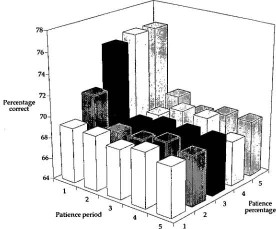
3.1.1 Description of node patience 38
3.1.2 Results and discussion 39
3.1.3 Need for hidden nodes 41
3.1.4 Summary 42
3.2 Alternative candidate node training schemes 43
3.2.1 Description of alternative candidate training methods 43
3.2.2 Experimental design 45
3.2.3 Results and discussion — single activation function 47 3.2.4 Results and discussion — multiple activation functions 50
3.2.5 Summary 52
4 Altering connection strategies within Cascade-Correlation 53
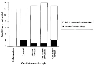
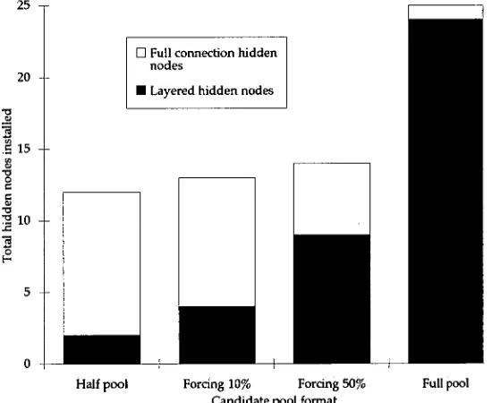
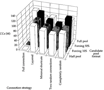
4.1 Limiting connections by growth 53
4.1.1 Alternative node connection strategies 54
4.1.2 Node forcing and experimental design 55
4.1.3 Results and discussion 56
4.1.4 Summary 61
4.2 Limiting connections by pruning 62
4.2.1 Pruning algorithm 62
4.2.2 Where to prune? 63
4.2.3 Stopping pruning 64
4.2.3 Summary 69
Part II Benchmarking Cascade-Correlation
71
5 Background to benchmarking databases 73
5.1 Features of data sets 73
5.1.1 Underlying problem structure 73
5.1.2 Factors affecting the data presentation 75
5.1.3 Inductive bias 79
5.2 Real-world and constructed data sets 80
5.2.1 Constructed data set benchmarks 80
5.2.2 Real-world data set benchmarks 83
5.3 Application of previous benchmarks 84
6 Real-world data sets — two new examples 87
6.1 Example one — ageing abalone 87
6.1.1 Initial data preparation 87
6.1.2 No hidden nodes 91
6.1.3 Hidden nodes 92
6.1.4 Optimal Performance 93
6.1.5 Confusion matrices 95
6.1.6 Pruning 96
6.1.7 Other classification methods 98
6.1.8 Summary 99
6.2 Example two — identifying authors 99
6.2.1 Details of author data 100
6.2.2 Full data Cascade-Correlation experiments 102
6.2.3 Cross-validation error estimation 103
6.2.4 Restricted attributes 104
6.2.5 Other methods 106
6.2.6 Summary and discussion 107
7 Constructing data sets — two methods 109
7.1 Voronoi data sets 109
7.1.1 Data set characteristics 110
7.1.2 Measuring complexity 112
7.1.3 Simulation results on Voronoi data sets 114
7.1.4 Summary 118
7.2 Normal data sets 119
7.2.1 Optimal classification 120
7.2.2 Simulation results on normal data sets 121
7.2.3 Summary 122
7.3 Application of benchmarks 123
7.3.1 Quickprop and back-propagation 123
7.3.2 Cascade-Correlation and modifications 127
7.3.3 Summary 130
8 Conclusion 133
Appendices 137
A Node patience results 139
B Candidate training results 145
B.1 Single activation function 145
B.2 Multiple activation functions 148
C Limited candidate node results 153
D Pruning results 159
E TasCas — a Cascade-Correlation simulator 167
E.1 Introduction 167
E.2 Network input I — data file 168
E.3 Network input II — simulator options 169
E.3.1 Weight training options (Quickprop) 170
E.3.2 Stopping training 171
E.3.3 Candidate training controls and options 172
E.3.4 Pruning and weight reduction 175
E.3.5 Obtaining network results 176
E.3.6 Trial options 176
E.3.7 Checkpointing and file recovery 177
E.4 Network output 177
E.4.1 Header Information 177
E.4.2 Final and summary results 178
E.4.3 Other outputs for completed training of a single trial 180
E.4.4 Progress during training 182
E.4.5 Regression results 183
E.5 Possible errors 183
E.6 Code structure 184
E.6.1 Module overview 184
E.6.2 Main training mechanism 185
E.6.3 Other code groups 185
E.7 Special considerations 186
E.7.1 Standard notation and indexing 186
E.7.2 Module specific considerations 186
E.7.3 Error and correlation formulas 187
E.8 Planned improvements 188
E.B Options summary 190
E.0 Full header information 192
E.D Complete examples 193
E.D.1 Example one 193
E.D.2 Example two 195
1 Introduction
In recent years there has been an enormous increase in the amount of research conducted in artificial neural networks. This may be loosely divided into two complementary areas: firstly, the application of computational methods to the development of realistic models of neural functions, and secondly the application of the distributed computation methodology to solving problems, not necessarily in a biologically plausible manner.
One of the most developed and researched areas in the applications part of artificial neural networks is inductive learning — the learning of a theory from individual examples presented to the system. In particular, supervised learning — where an answer is known and used to improve performance — is particularly popular. The back-propagation algorithm [Rumelhart, Hinton & Williams 1986] is easily the most frequently used artificial neural network model, not only because of its simplicity, but also because of its effectiveness at producing good solutions to a wide range of problems.
One of the difficulties with the back-propagation algorithm, and others like it, is that details of the network structure need to be decided prior to training. This requires a priori
knowledge of the problem to obtain good performance, gathered either from knowledge of the problem domain or from experimentation using the learning algorithm.
In response, attempts have been made to develop algorithms which change their internal structure as well as training the network weights, with the aim of removing the onus on the user of selecting the network topology. An artificial neural network which dynamically alters its topology, not only alleviates the need for human intervention, but also potentially gives extra flexibility which allows the training algorithm to more effectively find a solution [Baum 1989].
One of the more promising algorithms for dynamically altering artificial neural network topologies is Cascade-Correlation (Cascor) [Fahlman & Lebiere 19891. This algorithm starts with a minimal network architecture, to which hidden nodes are added as required, forming feature detectors within the network. The first part of this thesis examines this algorithm, extending the methods of training and examining further ways of altering the final network topology.
A further difficulty with the development of inductive learning via artificial neural networks is the frequent reliance on minimal testing to measure the performance of various
benchmarks for inductive learning systems. A large number of generated benchmarks are too simple to be realistic, and are thus not able to test the algorithms such as Cascor.
Hence the second part of this thesis examines the area of benchmarking supervised
inductive learning — in particular artificial neural networks. Two new real-world problems and two methods for generating complicated artificial problems are examined and assessed.
1.1 Organisation of thesis
To limit the size of this thesis it is assumed that the reader has background knowledge of inductive learning, particularly classification which involves the separation of examples into distinct classes; and supervised feed-forward artificial neural network methods.
The main body of this thesis is in two major sections. The first part involves alterations made to the Cascor neural network architecture in an effort to improve its performance. This consists of three chapters. Chapter 2 reviews methods of dynamically altering the structure of feed-forward fully-supervised artificial neural networks, and then details an outline into which all such algorithms fit. The chapter is concluded by giving a description of the Cascor algorithm, the parameters and data sets used, and the results of Cascor as applied to nine problems used for benchmarking the first part of the thesis. Chapter 3 examines methods for assisting and speeding the training process: a method used to halt training when little performance increase is being achieved; and alternative methods for training the candidate nodes. Chapter 4 examines methods of reducing the number of connections within a Cascor network — the aim being to produce a smaller classifier which will generalise at least as well and possibly better by using fewer free parameters. This is addressed in two ways: by the addition of hidden nodes which have a limited initial
connection strategy, and by the pruning of hidden nodes and the output layer to reduce the number of connections after a suitable amount of training is completed.
methods of generating complicated data sets, and their application to comparisons between various artificial network training methods.
Finally, Chapter 8 concludes the work in the thesis, and suggests further work which may be conducted in both the areas of examining Cascor and benchmarking strategies. Full details of the experiments undertaken in Part I are detailed in Appendices A through D. Appendix E is an abridged version of the manual for the simulator used to perform the Cascor
experiments [Waugh 1995cl, and Appendix F gives the complete bibliography.
1.2 Inclusion of papers
For clarity the papers which have been included within this thesis as part of the author's own work are outlined with references to the relevant sections. Firstly, those which have been accepted in refereed conferences are given:
[Waugh & Adams 1993] §5.3 [Collier & Waugh 1994] §5.3 [Waugh 8,z Adams 1994] §4.1 [Adams & Waugh 1995] §8.1
[Waugh 1995a] §3.1 and §3.2
[Waugh 1995b1 §7.1
[Waugh & Adams 1995] §4.2
Secondly, unrefereed works are outlined:
2 Background to dynamic learning
One of the major criticisms of fully-supervised feed-forward artificial neural networks is their failure to cope with requirements for different topologies. Usually only a simple, fixed network structure is used: namely one hidden layer with no shortcut connections, forming two processing layers. The problem is not due to the limitations of particular weight training algorithms, such as back-propagation [Rumelhart, et al. 1986], but rather is due to the limits of the network's structure and how this is developed [Baum 1989]:
... it is unlikely that any algorithm which simply varies weights on a net of fixed size and topology can learn in polynomial time. ... obstructions to rapid learning can be avoided if one considers algorithms with the power to add neurons and synapses, as well as simply varying synaptic weights.
An artificial neural network has a set number of inputs and a set number of outputs, as defined by the problem being addressed. However, the internal hidden connections, weights and nodes may be altered in any way by the training algorithm.1 This includes deciding what connections are present between nodes, whether there should be distinct layers of nodes, and so on. Overall, the number of free parameters, or the ability of a network to model further data set features, corresponds roughly with the number of connections [Cortes, Jackel & Chiang 1995]. Thus, the modification of network features allows for more parameters to be added to model the underlying data set function, or the removal of parameters to avoid over-specialisation on the given training data.
This chapter investigates the dynamic alteration of network topologies during the training of fully-supervised feed-forward artificial neural networks. It is suggested by many
researchers (for example, [Baum 1989; Fahlman 1990]) that dynamically altering networks presents good opportunities for developing optimal network architectures that generalise well. This chapter gives an overview of past methodologies, both constructive and destructive; gives a general reasoning as to why certain types of topology-changing algorithms are successful based on a framework developed from the literature; and concludes by giving a more detailed description of Cascor and introducing the remaining chapters in this part of the thesis.
1 In this thesis, the term connection is used to indicate the presence of a link between two nodes,
2.1 Current literature on dynamic neural networks
The main aim of dynamic neural network algorithms is to produce a network which effectively solves the problem at hand. This is done in two basic ways: by either removing unnecessary features to make the network smaller, or adding features to a minimal network as required. The fewer free parameters that exist in the network, the more likely that they will be correctly estimated from the available training data_ The greater the number of free parameters, the more likely the network will have the ability to model all of the data. Thus the task of the dynamic neural network algorithm is to produce the most appropriate number of parameters in a form which models the function underlying the data, without allowing for over-specialisation.
Few papers summarise the major construction and pruning strategies. Wynne-Jones concentrates on weight decay methods, and node construction and pruning — the paper does not examine the ideas of connection pruning in any detail [Wynne-Jones 1991a]. Hertz, Krogh and Palmer briefly examine connection pruning, weight decay and node construction algorithms [Hertz, Krogh & Palmer 19911. Reed gives a very good overview of the different pruning strategies, identifying the two main groups of pruning algorithms: sensitivity calculation methods, and penalty-term methods [Reed 1993]. Fiesler provides a very brief tabulated overview of many methods of changing topology within perceptron-style
networks and others [Fiesler 19941. The general perceptron-style topology altering methods are described more fully below.
2.1.1 Removing connections — saliency methods
There are two main ways of removing connections between nodes: by pruning using saliency measures, or by pruning using penalty-term methods to reduce weights to zero. Removing weights by the use of penalty terms will be considered in the next section.
The saliency of a connection is the change in error after the removal of that connection, or the sensitivity of the network to the removal of that connection [Mozer & Smolensky 1988]:
Saliency = Error (connection removed) - Error (connection present) (2.1)
Thodberg examines the removal of connections by a process of direct elimination: each connection is pruned in turn, and the resulting network is retrained for a short period [Thodberg 1991]. If the network still performs reasonably the change is kept, otherwise the connection is returned along with the original network weights. This method may be time consuming — to the point of being computationally intractable — but it has reasonable success in removing extra connections and.retraining existing ones. A saliency estimate is not calculated as the weights are individually removed, and the effect on the network is evident after training.
Skeletonization [Mozer & Smolensky 1988; Mozer & Smolensky 1989] is a technique which removes nodes by assessing the relevance of their connections. This process may be simply extended to the removal of connections, as it actually estimates the error after removing a single connection, which is combined to give the error after the removal of a node. Karnin notes that Mozer and Smolensky's sensitivity measure is defined to be used with a particular linear error measure, and he goes on to describe a sensitivity measure specifically for
network connections which is independent of the error function used [Karnin 1990].
Another sensitivity measure is Optimal Brain Damage (OBD) [Le Cun, Denker & Solla 1989] and the subsequent method Optimal Brain Surgeon (OBS) [Hassibi & Stork 1992]. OBD calculates saliencies by comparing the results of the main diagonal of a Hessian matrix, or the second derivatives, of the change in error with respect to the weights. A Taylor expansion of the error results in four groups of terms: the first term is assumed to be constant, the second term is assumed to be zero as the network has been trained to a local minimum and the slope is constant, the third term results in the Hessian matrix which calculates the quadratic approximation or curvature of the error surface, and the higher order terms are ignored and assumed to be negligible. The main diagonal of the Hessian matrix gives an estimate of which connections are required. OBS follows this up with improvements, mainly by using the full Hessian matrix, in contrast to using only the diagonal. This has the advantage of requiring no retraining after the changes have been made whereas OBD does require retraining. Nevertheless, these computations can be quite expensive. A number of papers have examined these algorithms further, with comparisons between OBD and OBS, and some improvements and modifications to the algorithms — particularly to the OBS algorithm (for example, [Gorodkin, Hansen, Krogh, Svarer & Winther 1993; Hassibi, Stork & Wolff 1993; Tolstrup 1995]).
claims that PCP is likely to produce better results than OBD, although this is not backed up with results.
Another method [Tsaptsinos, Mirzai & Leigh 1992] uses correlation analysis for the removal of unnecessary connections; and there are a number of papers which optimise the network architecture by using genetic algorithms (for example, [Nolfi & Parisi 1991; Hancock 1992; Kendall & Hall 1992; Kendall & Hall 1993]), though it is not obvious from the papers that this is an efficient process, especially for larger networks [Hertz, et al. 1991].
Sensitivity measures also have their critics [Reed 1993]:
... most of the sensitivity methods ... don't detect correlated elements. ... An extreme example is two nodes which cancel each other out at the output. As a pair, they have no
effect on the output, but individually each has a large effect so neither will be removed.
Retraining may break such a deadlock, but this will not necessarily result in an optimum solution.
2.1.2 Modifying weights — penalty terms
Another way of removing a connection, as mentioned previously, is by changing the weight of that connection so that the connection has no effect. Pruning of weights, or regularisation, is performed by adding a penalty term affecting the network complexity to the network error term which is being minimised, with the purpose of changing the magnitude of the network weights. With this method generally weights are reduced to remove their effect. This relies on the weight training algorithm to reduce the weights by minimising the overall network cost:
Network cost --- Network error + Network complexity (2.2)
The minimisation of the overall cost results in the training of the network weights and the alteration of the weights to minimise the term specifying the network complexity.
Weight decay and weight elimination are mentioned quite extensively in the literature. Less frequently mentioned is the use of weight enhancement to generate weights from zeroed connections [Chauvin 1988].
weights in the network. Hanson and Pratt, and Burkitt and Ueberholz also examine this method, with the latter attempting to separate the learning from the weight reduction phases [Hanson & Pratt 1988; Burkitt & Ueberholz 1993].
Weigend, et al. propose a system for weight elimination which subsumes much of the work done in weight decay [Weigend, Rumelhart & Huberman 1990; Weigend, Rumelhart & Huberman 19911. This system, similarly operates by training to a set minimum error for a particular problem and trades off complexity and the network error. The method allows for the alteration of the weight cost function so that smaller weights or larger weights become relatively expensive.
NowIan and Hinton describe a further penalty term method called soft weight sharing [Nowlan & Hinton 1992]. Under this scheme an alternative penalty term is used which favours the reduction of smaller weights. The penalty term involves the combination of two Gaussian functions. One function is used to reduce the smaller weights, while the other targets larger weight values — the latter, in the limiting case, may be replaced with a uniform distribution. The penalty term is reduced by allowing the means and variances of the Gaussians used to adapt such that the variances shrink, drawing the weights into having similar values, which in turn implements a 'soft' version of weight sharing, whereby asingle weight is used by several connections. By starting the penalty-term Gaussians with high variances, all the weights influenced by the respective Gaussians will be forced to have similar values. The wide variance at the beginning means that the Gaussians will not adversely affect the training process. The sharing of weights results in a reduction of the degrees of freedom that the network may use for over-fitting the data. There is, of course, a greater cost with the increased complexity of the weight optimisation process.
Not everyone is in favour of these penalty-term methods. Mozer and Smolensky state [Mozer & Smolensky 19891:
... our impression is that it is a tricky matter to balance a primary and secondary error term against one another.... In our experience, it is often impossible to avoid local minima — compromise solutions that partially satisfy each of the error terms.
2.1.3 Changes to the number of hidden nodes
The large majority of papers with respect to topology altering algorithms consider changes in the number of hidden nodes, rather than changes to the connections or weights between nodes. Most of these papers concentrate on the introduction of new nodes when the network is not capable of solving the problem at hand. Only a few examine the removal of nodes. These different styles will be considered in turn.
2.1.3.1 Construction — adding hidden nodes
Many techniques are based on the standard configuration for a back-propagation style of network, with two layers of processing nodes. The idea of splitting nodes in the hidden layer, or simply adding extra nodes to the hidden layer is very common (for example, [Ash 1989; Hanson 1989; de le Maza 1991; Platt 1991; Refenes & Vithlani 1991; Wynne-Jones 1991b]).
Several methods have been developed which grow layers as well as the number of nodes in a single layer. The majority have been designed for problems with binary inputs, but could be extended to cover more general cases. Gallant presents three concepts of network growth which involve the addition of individual nodes [Gallant 1986]: growing nodes with
connections to the previous node and the inputs (Tower Construction), growing nodes connected to all previous nodes and inputs (Inverted Pyramid Construction), and adding static nodes in layers. No results are given as to the effectiveness of these ideas. The Tiling algorithm [Mezard & Nadal 1989] builds another layer on the network outputs if the previous layer does not separate the classes in the problem. Along a similar vein is the Extentron algorithm [Baffes & Zelle 19921 which forces the separation of examples by
extending a standard perceptron. The Upstart algorithm [Frean 1990] produces a binary tree of nodes which correct the values of the outputs for all training examples, the purpose being to correct any mistakes by adding extra positive and negative signals to the output node. This adds as many nodes as required to correct the error. The Upstart algorithm performs better than the Tiling method [Wynne-Jones 1991a], however both suffer from the limitation that only binary tasks are addressed.
Cascor is not limited to binary problems nor to a certain number of layers [Fahlman & Lebiere 1989]. It allows the addition of hidden nodes as required which have connections from all previous hidden nodes and the inputs, and are connected in turn to all outputs — hence giving the Inverted Pyramid Construction identified by Gallant. The network starts as a single output layer with full connections between the network inputs and outputs.
candidate nodes. The node with the highest correlation to the network error after the candidates have been trained is installed. The weights of this hidden node are then frozen and the output layer is retrained with the extra node connected to it. This process is cyclical and continues until either the training set is classified correctly or the maximum number of hidden nodes has been added. This produces all possible feed-forward connections, and the ability of hidden nodes to connect to other hidden nodes allows for the possible formation of advanced feature detectors. The Cascor algorithm has been extended a number of times [Littmann & Ritter 1992; Simon, Corporaal & Kercichoffs 1992; Simon 1993] .
One limitation of Cascor is that it is not effective when examining regression style problems. The correlation machinery tends to over-compensate which means that the results, though effective for classification, tend to over-shoot on regression problems [Fahlman 1993; Hwang, You, Lay & Jou 1993; Freeman 1994; Adams & Waugh 1995].
Projection Pursuit Learning (PPL) [Hwang, et al. 1993; Hwang, Lay, Maechler, Martin & Schimert 1994] involves a single hidden layer of nodes with adaptable activation functions. Nodes are added to the single hidden layer when required, and the activation functions are altered to solve the required problem, rather than adding more nodes with fixed activation functions to a deepening network as with Cascor. Simulations indicate that PPL is
extremely effective at solving regression problems, as the activation functions adapt to fit the shape of the problem structure.
2.1.3.2 Pruning — removing hidden nodes
Three main methods are employed for node pruning: heuristic solutions, saliency measures which are extensions of the methods used to prune connections, and node decay based on weight decay methods. Sietsma and Dow take the heuristic approach by comparing nodes based on the network outputs of all training patterns [Sietsma & Dow 1988]. The idea is to remove those nodes which have little effect — non contributing units; or whose effect is duplicated by other nodes — the unnecessary-information units. It also removes layers by determining if they are redundant. Shamir et al. consider the reduction of hidden nodes by merging neurons with similar functional behaviour, hence preserving functionality [Shamir, Saad & Marom 1993]. Statistical results are presented to support the algorithm. Chung and Lee also develop a node pruning algorithm which removes four styles of unnecessary nodes: non-contributing, duplicated, inversely-duplicated and inadequate nodes [Chung & Lee 1992].
irrelevant [Segee & Carter 1991]. Ramachandran and Pratt extend the Skeletonization idea by basing a node pruning method on an information measure from the inductive learning literature [Quinlan 1986b; Ramachandran & Pratt 19911. Similar ideas are presented by Dunne et al. with regard to nodes which attempt to separate only one class from the rest of the classifications in the problem [Dunne, Campbell & Kiiveri 1992]. Adams and Jones also examine a node's relevance in relation to function interpolation with success in creating minimal single layered networks [Adams & Jones 1992].
Chauvin examines the removal of nodes by a weight decay method which is altered to encompass all weights connected to the one node, rather than operating on individual weights [Chauvin 1988]. Ji et al. also consider the removal of nodes using a penalty term, along with the reduction of weight magnitudes at the same time [Ji, Snapp & Psaltis 1990].
2.1.4 Combinations of different strategies
As the methods mentioned above may be applied in different phases of network training, combinations of different methods have occurred. Sietsma and Dow examine one method which combines the use of growing and pruning algorithms [Sietsma & Dow 1991]. One deficiency with their method of heuristic pruning [Sietsma & Dow 1988] is that although it may produce a minimal number of nodes in a layer, the output of the layer may not be linearly separable. This may require the introduction, and hence growth, of extra hidden layers to overcome the newly created problems with the hidden layer or layers. The result is a transformation of a wide and shallow network into a thin, deep network which may generalise better than the originally trained network. The problem is that this method is used over and above the training of the initial network, thus increasing the time required for training.
Wynne-Jones favours the combination of constructive algorithms and pruning methods to overcome the problems of obtaining the minimal network, by allowing the training process to increase the size of the network, and then reduce it when the task has been learnt [Wynne-Jones 1991a]. No specific system is presented in the paper. There have been algorithms developed which both add and delete hidden nodes from a single layer (for example, [Murase, Matsunaga & Nakade 1991; Wang & Hsu 1991]).
There are a number of additions to the Cascor algorithm to include further topology
2.1.5 Further comments
In the case of using pruning algorithms, where initially excess connections or nodes are in the network, often the extra free parameters aid in the learning process as well as the speed of learning [Mozer (Sr Smolensky 1988; Izui 8r Pentland 1990; Thodberg 1991; Wynne-Jones 1991a].
Not all people agree with this approach [Ash 1989]:
There are some shortcomings to the pruning approach. Since the majority of the training time is spent with a network which is larger than necessary, this method is computationally wasteful.
This training speed problem does not occur with methods such as Cascor [Fahlman 1993], as it seems to be related to the 'herding' problems that have been identified within standard back-propagation style networks [Fahlman & Lebiere 19891. Since in back-propagation all hidden nodes are active at any point in time during the training of the hidden layer, all the nodes are trying to correct the same error. To ensure that a solution is reached, a greater than optimal number of hidden nodes is required for training to ensure that the nodes are well spaced by the initial random allocation of weights. Cascor, for example, does not suffer from this problem as only one hidden node is trained at a time so that the maximum error is reduced by one node and then its weights are frozen. Nevertheless, it is not guaranteed that this 'greedy algorithm' will produce a minimal network [Fahlman 1990], as it is trying to remove as much of the error as possible using a single hidden node.
A further criticism of pruning is that the reduction in the number of connections may lead to
a corresponding reduction in the fault tolerance of networks, inherited from the way in which knowledge within the network is distributed. Work done on the effect of pruning on the fault tolerance of networks indicates that after pruning a network's ability to cope with being damaged is not decreased [Segee & Carter 1991]. This should be taken in the context that generally, back-propagation gradient-descent trained networks do not have significant fault tolerance capability, as usually individual weights may have a great bearing on the end result [Bolt 19921.
0
0
0 0
0
2.2 Abstraction of topology changing methods
This section outlines an abstraction of possible ways of changing network topologies developed from the literature presented above. Feed-forward networks can be considered to be directed acyclic graphs. There are two features of a general acyclic graph: the set of vertices, and the set of directed edges between those vertices. Artificial neural networks can be mapped to acyclic graphs such that nodes are regarded as the vertices, and connections being the directed edges. The weight of a connection can be considered to be a strength of the directed edge. From this it can be seen that there are two general topological features of artificial neural networks, namely the nodes and the connections with their associated weights. The distinction between connections and weights may be considered to be arbitrary, but it reflects a difference in methods presented in the literature.
Disregarding whether nodes, connections, or weights are being examined, there are three common ways in which topologies are altered: by the use of constructive algorithms to add features to the network, using destructive algorithms which remove or prune features from the network, and a combination of constructive and destructive algorithms. Any algorithm which considers the alteration of a network topology will then be adding or removing nodes, connections, or weights. These will be considered in turn below. Note that if a node is added or removed, so are all the connections to that node, so changes which include whole nodes amount to the addition or removal of blocks of network connections.
2.2.1 Changing connections and weights
Firstly, adding or removing connections or weights is examined. Consider that there are ii potential inputs to a particular node, then there are 2n possible connection strategies to that node (see figure 2.1). In a construction algorithm, a base case of minimal connections to a node is needed to which new connections can be added. As the number of inputs to a node increases, the number of possible starting connection strategies to that node increases dramatically. The large number of possibilities would mean that the best initial connection strategy would often be missed if only a few were selected randomly. Though there are advantages to having nodes with limited fan-in, the large number of combinations make their use prohibitive.
For example, consider the case where each node has a maximum of two connections. If there are n network inputs there will be:
n! (2.3)
2 • (n ±2)!
possible node connection strategies to the input layer, without even considering the need to train multiple nodes with different random weights to avoid local minima. Therefore for 10 inputs, there would be 45 different connection strategies for each node to be used.
It may also be possible to employ some form of weight enhancement to add in connections when they are required from zeroed weights. The problem of what is a sensible initial connection strategy comes up again, as most weight training methods require the setting of random initial weights. If a network required the majority of weights — or all weights as is the obvious choice — to be set to zero, allowing weight enhancement to be employed at some later stage, there will be little variation to avoid local minima. Further, it is difficult then to start the training process and decide which weights should be allowed to vary.
A pruning algorithm for connections would start at the more obvious position of all possible connections to a node being present and could then decrease the number of connections • according to some pruning strategy. Although there are the same number of possible connection strategies, a unique base case exists to start training on, and it is easier to remove connections which have no effect than add connections which may have an effect. Likewise, weight decay methods seem more reasonable than weight enhancement as they can
gradually reduce weights that are already in place. One concern with choosing a pruning , approach is that initially training the extra connections would require more computational time for little gain than a more limited connection strategy, especially when a large number of connections are redundant.
2.2.2 Changing the application of hidden nodes
Finally, additions and deletions to the number of hidden nodes are considered. Whereas the number of connections has an upper limit set by the maximum number of inputs to the particular node, the number of hidden nodes has no upper limit. The base case is naturally no hidden nodes at all — perhaps forming just a perceptron-style output layer. Thus a node construction algorithm seems quite attractive as long as the initial conditions are sensibly set. This will require at least one node in each hidden layer or some strategy for forming new layers.
the initial topology needs to be decided: what is the maximum number of hidden nodes required, how many layers are needed and how are the nodes to be connected to proceeding and succeeding layers. A sensible possibility would be to start with a fully connected layered network and remove unnecessary nodes. This relies on the weight training, possibly over a large number of layers, to find a reasonable solution in the first place and also to be reasonably quick; and puts the onus on the user to allocate the initial topology to be just larger than the necessary final network, to reduce the overall training time.
Thus the most promising approaches seem to be to add hidden nodes and remove
connections. The ideal of using the smallest number of layers may also be incorporated into this scheme if this is judged as being important for the network application. This abstraction is mirrored by the methods presented in the literature.
2.3 Standard Cascade-Correlation
Cascor is examined as one of the most promising node construction algorithms, as it is able to develop networks with multiple layers creating advanced feature detectors, and it is able to examine problems with real-valued inputs. Its real strengths lie in the area of
classification where the outputs are binary and it is this excellent performance which warrants further consideration. The algorithm's performance with real valued outputs is less than optimal [Adams & Waugh 19951. Furthermore, it is a prime candidate for the use of methods to reduce the number of connections, as the algorithm adds hidden nodes with all possible feed-forward connections, many of which may be redundant. This leads to a natural combination of growing and pruning methods, in line with the trends evident in the literature.
2.3.1 Overview of Cascade-Correlation
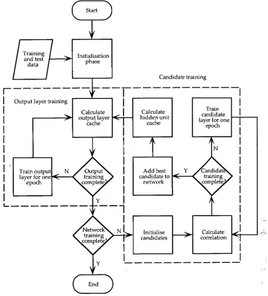
The Cascor algorithm cycles between two phases to train a network: the first phase involves training and further retraining of the weights to the output nodes; and the second involves the gradual addition of hidden nodes to the network (see figure 2.2). The second phase is the more complicated whereby candidate nodes are trained to maximise their correlation with the network error, and the best of these nodes is installed into the network.
Training and test
data
Initialisation phase
Candidate training
Output layer training
Calculate output layer
cache
Train output
layer for one
<
epoch
L
Calculate hidden unit
cache
Add best candidate to
network
Initialise candidates
End )
Calculate correlation
(
[image:27.565.119.507.45.474.2]Start
Figure 2.2 — Flow-chart outlining the Cascor algorithm
2.3.2 Output layer training
Cascor starts developing a network by initially training a layer of weights between the input nodes and the output nodes. This single layer is fully-connected and prescribed by the problem and data representation chosen. The output layer configuration, with random weights set during the initialisation process, is trained to produce a minimal error (see §2.3.5).
For efficiency and speed considerations the training process initially involves caching the required values from the evaluation of the network: namely the network outputs for each example, the error values for each output and example and the overall network error. The error for each output and example value is as follows:
ekp = y kp ± tip (2.4)
where ekp is the error over all outputs k and all training patterns p, ykp is the output node value and tkp is the expected output value.
The output and error values are cached for later use in the training process, especially during the training of the candidate nodes where these values are not altered over several iterations. The caching is not necessary, but it greatly speeds up training if the machine memory is available. Otherwise the values and errors of the output nodes must be recalculated for each example when required.
Once the values have been cached, it is possible to say whether the goals of training have been met, as the most recent network has been evaluated. At this point it is decided whether training the output layer should continue. This process is described more fully below (see §2.3.4). If these goals have been met — which is unlikely if no changes have been made to the weights — then the output layer training phase is complete. If this does not occur then the output layer weights are trained using Quickprop (see §2.3.5) and the algorithm cycles to evaluating and caching the output layer information. This process continues until training of the output layer is considered to be complete.
The error to be back-propagated (3) is calculated as follows:
Skp = f kp • ekp (2.5)
error calculations within the experiments presented within this thesis. The learning error rate used is:
T1 (2.6)
where n is the nominal learning rate and t is the total number of training examples. This scaling is for the benefit of Quickprop to keep the updates within a sensible range.
Once the output layer training is complete as mentioned previously, the algorithm checks to see if the conditions of training the entire network have been met (see §2.3.4). If they have, the algorithm stops, otherwise candidate units are trained and one of those units is installed in the network. The output layer is then retrained with connections to this new hidden unit, and the process cycles. The process of training the candidates is described next.
2.3.3 Candidate training
The training and installing of a hidden node is performed in a similar manner to the output layer training: a number of candidate nodes are given initial random weights, and they are then trained independently to maximise their correlation to the network error; the total number of candidates is specified by the user. The candidates are connected to all the input nodes and all the previously installed hidden nodes.
The training cycle for candidate nodes begins by calculating the correlation2 of each candidate node with the residual error at the output nodes. The original Cascor paper [Fahlman & Lebiere 1989] gives the following formula for the correlation calculation (S) for which is to be maximised each candidate:
S =
k = 1
E
(v,,,±cle kp±p=1 ' (2.7)
where vp is the value of the candidate for example p, and z) and ëj are the averages of the candidate values and the errors for each output respectively. This results in the following derivative with respect to the candidate's input weights which are being trained:
DS _ G ekp ± Fk) f • x,F,
-k=1 k p=1( r
(2.8)
where o-k is the sign of the correlation between the candidate's value and output k, xip is the input the candidate receives from the unit i for the pattern p, j is the index for the candidate nodes, and wi is the weight to the candidate from the input layer. The unit i may be a network input or a previously installed hidden node. In the actual implementation released by Fahlman, and the subsequent TasCas simulator [Crowder & Fahlman 1991; Waugh 1995c1 error normalisation is implemented for correlation values. This amounts to having the following formulas instead of (2.7) and (2.8):
=1 s -
k p=1 VP .ekP tv. k
(2.9) m t
I ek 2
k=lp=1
±ak • ± (ekp • fip
=
as k=i p=1
k=lp=1
These formulae are used for the calculation of the correlation and the subsequent modification of candidate weights within the candidate training process.
If, as calculated from the correlation calculations, training is not complete (see §2.3.4) then the candidate node weights are modified by gradient ascent to maximise their correlation with the output nodes. The learning rate is normalised in a similar manner to the output layer training rate to keep the Quickprop updates within a sensible range [Crowder & Fahlman 1991]:
11
t-(n+h-F 1) (2.11)
where n is the total number of inputs, and h is the number of hidden nodes installed so far, and n again is an arbitrary constant representing the learning rate.
Once the candidates are trained the candidate with the largest correlation is installed in the network. Its input weights are added to the network and frozen so they will not be altered. The freezing is effected by only training the output layer weights during the output training phase, and not back-propagating the errors past the output layer. The output layer weights for the newly installed hidden nodes are set using minus the last correlation calculated as an initial guess (—S). Fahlman has found this to be more effective than just setting random weights [Fahlman 1993]. The hidden unit cache may then be updated with the values produced by the new hidden node. As the hidden node weights are frozen, these will not alter during the rest of training.
1p
The output layer is then retrained with the newly installed hidden node as an extra input to all the output nodes. This process cycles, adding in further hidden nodes, until the training is completed. The extra connections to the previous hidden nodes generate a very deep network with one node per hidden layer and all possible shortcut connections installed. The maximum number of hidden nodes which can be installed is again specified by the user.
2.3.3.1 Correlation derivation
The following is the derivation of the correlation S with respect to the candidate's input weights [John 1995]:
as _ k=1 p=I (Vp rlekp
DTATi dWi
t (
a
1
X1 ±
V)(ekp ±k=1
a ± (
v to ±v)(ekp ±Fk)where ak is the sign of the correlation = k =I GI( aw;
± qekp ±
= E k=1 ak p = I awi
a(vp±v)
= ak I (ekp ± -e7,) as ek does not depend on VV,
k=1 p=1 Lovvi t
= k1 akpI= 1 (av
P 7-v
Tv
■
Ti (ekP ±DN'7;
The error is independent from the candidate weights as this is dependent on the output weights only. From the definition of the network:
n + h
Vp = W. • X• ip 1=1
the following may be calculated:
n + h
Dv af(E w • xip) ,.1
= awi
n + h
(
a w; • xip)
= f' dwi
= f' •
which may be used within the last equation of (2.12) to give:
as
_ (f,
_k=1 —kp„ u. • Xip f xi)(ekp ± Fk)
(2.12)
(2.13)
(2.14)
This formula can be shown to be equivalent to the original calculation of the derivative (2.8) as the f' • x, term sums to zero. Removing this additional term may lead to some problems of precision, although empirical evidence does not indicate that this has had any major effect [John 1995].
2.3.4 Stopping Training
There are three points within the Cascor algorithm where decisions need to be made as to whether training should continue. These are at the end of each output layer training epoch, at the end of each candidate pool training epoch, and for the entire network at the end of each output layer training phase.
At these different points different methods are used to decide when training is complete: • an arbitrary limit — which is used for output layer and candidate training
setting a maximum number of epochs which training may take, or is used by the overall network training by setting the maximum number of hidden units which may be installed;
• a correctness limit — which is used for stopping output layer training and the entire network training; and
• a patience limit — which is used to halt output layer and candidate training when training is not resulting in an effective improvement in network performance.
If any one of these limits is met on a phase of training in which it is being employed, then training halts. Thus if, for example, the epoch limit is met on output layer training, then training halts regardless of whether the patience limit or correctness limit has been met. The arbitrary limit, irrespective of whether it measures the number of hidden nodes or the number of epochs, is a rough measure of training time; hence this may be regarded as a time limit.
The correctness limit is determined in two ways. The first is more appropriate for
classification problems, where a minimum number of error bits is set for a goal of training and often this minimum is set to zero. An error bit is where a value for an output for a particular example is outside a specified range, and is hence considered to be in error. This is counted as one error bit. If the number of error bits is zero then 100 percent correctness is said to be achieved. The maximum number of error bits is therefore the number of training examples multiplied by the number of outputs. The allowable range from the expected value is specified by an error threshold. Thus, for example, if a symmetric sigmoid
then a correct maximum value will be between 0.1 and 0.5, and a correct minimum value will be between —0.5 and —0.1.
The second method for judging correctness, which is more appropriate for regression problems, is to simply set an arbitrary error value which the network error must fall below:
(ykp tkp)2
MSE k = I P = i
m • t (2.16)
Fahlman provides further normalisation of this value within the released simulator (see [Crowder & Fahlman 1991] and §E.7.3).
Patience is a measurement of minimal activity specified by the two patience parameters: • patience error — the change in error required over a set period to continue
training; and
• patience period — the period over which the change in error is measured.
Thus if there has not been a change in the network error greater than the patience percentage of the error given — or the maximum correlation for training the candidate pool — over the patience period, then the network runs out of patience and that phase of training is
completed. The code for implementing the patience calculation is given in figure 2.3.
initialise by:
quitpoch = currentEpoch = 0; stillPatient = true;
At the end of each training period:
/* note that currentEpoch++ has occurred and currentError is set */ if (quitEpoch == 0) {
lastError = currentError; quitEpoch = patienceLength; ) else
if (fabs(currentError - lastError) > patiencePercentage * lastError) lastError = currentError;
quitEpoch = currentEpoch + patienceLength; ) else
if (currentEpoch >= quitEpoch) stillPatient = false;
At the completion of training:
totalEpochs += currentEpoch;
2.3.5 The Quickprop algorithm
Quickprop is the name given by Fahlman to a quasi-Newton method of minimising a function using an heuristic estimate of the curvature of the error function to improve performance over gradient descent back-propagation [Fahlman 198843 Any function can be expanded about a known point in a Taylor series. For simplicity consider the one dimensional case:
c
+ h2
2
'a
x
2 xof(x0 + h) = f(x0) + (2.17)
x0
The first term is proportional to the function evaluated at the known point, the second to the first derivative evaluated at that point and multiplied by the distance from it, the third to the second derivative evaluated at that point and multiplied by the square of the distance from it, and so on.
If the expansion is about a minimum, the curve in the vicinity of the minimum can be reasonably approximated by a constant and a term quadratic in the distance from the minimum, h. This is because the first term gives the value at the minimum, the second term is proportional to the slope of the curve which at the minimum is zero and the third term is proportional to the curvature at the minimum. At the minimum the curve is symmetric and hence all the terms proportional to the odd powers of h are zero. If h is small then even terms of order h4 and higher will be small compared with the quadratic term.
In minimising the error function in back-propagation this analysis cannot be directly applied since the position of the minimum is what is required rather than what is known. However, if near a minimum it is reasonable to take the shape of the surface to be quadratic. Fahlman makes the assumption that the surface is quadratic but applies it at all times rather than only near a minimum [Fahlman 19884 Fahlman makes the further 'risky' assumption that the weights are independent, thus changes to a weight do not affect the other weights in the network. The use of the partial derivative is the implementation of this assumption.
The standard gradient descent weight change, including the momentum term which need not be used, is as follows:
Aw(t) = tri • s(t) +a • Aw(t ± 1) (2.18)
3The technical report referenced here is available by ftp. The published version of the paper [Fahlman
where ri is the learning rate, a the proportion of momentum used and s(t) is the slope at time t. The Quickprop algorithm essentially changes this to:
Aw(o = s(t+4.00,406,w(t±i) (2.19)
leading to a crude approximation of the optimum value which gets increasingly better as the minimum is approached. The derivation of this is outlined below.
2.3.5.1 Derivation of Quickprop update
In back-propagation style networks the error function is a function of the weights and each weight is dealt with individually. At each step in the iterative process of minimising the error function the value of the error and the gradient of the error function at that point are known. Quickprop uses the current and previous gradients and the values of the weights to estimate the position of the minimum based on the quadratic approximation. Figure 2.4 illustrates the situation.
lAi 1A Wm W
Figure 2.4 — The error function, E is a function of a weight, w. At wi and w2 the gradients of the
curve are si and s2 respectively. wm is the position of the minimum
The error function is assumed to be a quadratic function of the weight, w, namely
E = a + bw + cw2 (2.20)
The slope of this curve is given by:
E
= b + 2cw (2.21)Two points are known, namely
D-TAE -i- = s, at w = w, and ..' E A., = s2 at w = w, (2.22)
= 0 at w = w,,, (2.23)
Substituting (2.22) into (2.21) we have:
s, = b + 2cw, and s2 = b + 2cw2 (2.24)
from which we derive:
b = slww22 ±± ws2w: and c = 2 w2± 1 s2± s'
Substituting these values into (2.21) and (2.23) we have: lb
wrn =
—± s, ww2 2 ± s ±w2w, 1 12 w2 ±w1 • 2 s2
s2w1 ± s1w2
s2 ± s,
Finally, if we interpret the subscripts to mean that wi and si are measured at time (t - 1) and w2 and s2 at time (t) and introduce two further parameters:
Aw(t) = Wm ± w2 and Aw(t ± 1) = w2 ± WI (2.27)
we can rewrite (2.26) as:
Aw(t) = s(t ±s(i)t) sw± Avs(t ± 1) (2.28)
which is the derived Quickprop formula [Fahlman 19884 Since it involves the (reciprocal of the) difference of two gradients divided by the distance between them, Fahlman is able to claim that this is an approximation to a second order algorithm.
2.3.5.2 Practical considerations
Since at a point a great distance from a minimum the quadratic assumption may be poor Fahlman has introduced a series of heuristic rules to deal with the cases where this assumption does not work well.
At the beginning of the training there is only one value of w and s known and hence simple gradient descent with learning rate TI is employed as the full Quickprop update formula will be ineffective. Likewise when the previous weight change is zero, gradient descent is used to continue the training process if required.
Furthermore, the standard gradient descent term is added to the Quickprop quadratic update if the current slope will cause the weight to move down the error slope in the same
(2.25)
direction as the previous change, helping to push the value toward the minimum. This additional term is not used if the slope changes: hence the weight is near the minimum where the quadratic weight update should be most effective.
lithe current slope is close to or larger than the previous slope and moving in the same direction — unlike the parabola that Quickprop formula models — a jump to the minimum may result in an overly large step. To avoid this Fahlman introduces a term 1.1, the maximum growth factor, to limit the step size. In such a situation ji times the previous weight change is used instead of the Quickprop update formula, where Fahlman suggests a value of 1.75 for This or the Quickprop formula are thus only used if the previous weight is non-zero.
A shrink factor is calculated from ji to test if the current slope is as large or larger than the previous slope. This is used to avoid taking steps which are too large. The shrink factor is defined as follows:
shrink factor = 1 +
Finally a weight decay term is added to the slope prior to these calculations to limit the growth of the weights, if required, giving the following cost function for the output layer as an example:
n
E = Eo +1,yi f
k=1 i = 1 k' (2.30)
where y represents the strength of the weight decay. A small decay value will ensure that the weights do not grow too large, for both the output layer and candidate weights.
All these modifications lead to the implementation shown in figure 2.5. For stability considerations this algorithm only works as a batch training method, which requires the presentation of a group of examples to update the weights. In this case each batch is considered to be a complete run through the training set, after which the errors are used to update the weights.
An offset to the activation function derivative to stop this getting close to zero, is also often employed in conjunction with the Quickprop algorithm [Fahlman 19884 Briefly the activation function offset adds 0.1 to the derivative of the activation function it is applied to. The purpose of this is to ensure that the derivative does not become close to zero for values at the extremes of the activation function. The weight update, by definition, is multiplied by the derivative, and thus there is no update if the derivative is zero or is near zero. This increases the effect of any error in the region of the activation function. In Cascor an activation function offset is used in training the output layer, but no activation function offset is used with the candidate nodes as this confuses the correlation machinery [Fahlman
Lebiere 19891. Adams and Lewis have shown that for function evaluation, which is related to finding the maximum of the correlation, the use of the offset is not useful.
nstep = 0.0; s += decay * w; if (pd < 0.0) {
if (s > 0.0) nstep -= eta * s;
if (s >= shrink * ps) nstep += mu * pd;
else nstep += pd * s / (ps - s); ) else if (pd > 0.0) {
if (s < 0.0) nstep -= eta * s;
if (s <= shrink * ps) nstep += mu * pd;
else nstep += pd * s / (ps - s); ) else
nstep -= eta * s;
pd = nstep; w += pd; ps = s;
Figure2.5— the C code for a single weight Quickprop update: s is the current slope, ps the previous
slope, pd the previous weight change, w is the actual weight, eta is the learning rate, mu the maximum
growth factor, decay is the weight decay term, shrink is the shrinkage factor, and nstep is a variable for
calculating the next step by the Quickprop algorithm
2.3.6 Diagrams
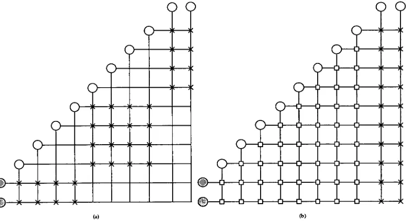
Since Cascor is able to install a large number of shortcut connections the usual layered network diagram becomes unmanageable and unable to convey the full network information. To overcome this problem Fahlman and Lebiere developed an alternative diagram for displaying cascaded neural networks [Fahlman (SE Lebiere 1989]. Examples of networks — both a standard layered network and a Cascor network — are given in figure 2.6. The shaded nodes are the non-processing inputs, and the nodes at the top of each diagram are the outputs. The boxes indicate frozen hidden node connections within the Cascor network and the crosses indicate trainable connections: for the Cascor network this involves only output layer connections. The vertical lines to a node indicates the nodes' inputs and horizontal lines from a node indicate outputs from that node. If no box or cross occurs on the intersection of a horizontal and a vertical line, then the relevant connection is not present. This method of displaying artificial neural networks is useful for displaying any variety of feed forward network.
2.3.7 Summary
• •
UNE
UNE.
I
me•
i
U
sumem
• mn
im
omm
•nomenou•
Wo
m
mommos
1111111111•1111•
• •
..S
sons
• sir•m
,Mom
• .20.11.100
siti••io•s
•OINIMIIEN
Ainituteasini
[image:39.563.104.513.42.265.2](b)
Figure 2.6 — Examples of (a) a standard two hidden layer network, and (b) a standard Cascor network • ri — the learning rate;
• p. — the maximum growth rate which limits the size of any change in weights
performed after each presentation of the training set; and
• y — a standard weight decay parameter which may be used to ensure that the
weights do not grow excessively large.
Once progress is no longer made, the maximum number of epochs of training has been
performed or the network achieves a correct result, output training is complete. If this
results in a correct network, or the maximum number of hidden nodes has been installed,
then the network training is complete. Otherwise a pool of candidate nodes is trained to
maximise their correlation with the residual error of the network. When the maximum
number of epochs has been reached or no progress is been made in the training of the
candidate nodes, the best candidate node is installed into the network and the output layer
is retrained. The algorithm thus cycles through installing hidden nodes and retraining the
output layer, and these phases themselves cycle through training regimes. The user of
Cascor has to decide what parameters to use for the specific application of the algorithm.
2.4 Experimental design
This section provides more specific details regarding the design of experiments throughout
this thesis. The assumptions and general algorithm parameters used for experiments are
given, followed by how network and general classifier performance is measured. The data
sets employed to test the ideas presented in the first part of the thesis are then outlined, and
finally details of the results of basic simulations using these data sets and parameters with
standard Cascor are presented. Modifications to the Cascor algorithm are presented in the