The Astronomical Journal, 142:60 (35pp), 2011 August doi:10.1088/0004-6256/142/2/60
C
2011. The American Astronomical Society. All rights reserved. Printed in the U.S.A.
THE PALOMAR TRANSIENT FACTORY ORION PROJECT:
ECLIPSING BINARIES AND YOUNG STELLAR OBJECTS
Julian C. van Eyken1, David R. Ciardi1, Luisa M. Rebull2, John R. Stauffer2, Rachel L. Akeson1,
Charles A. Beichman1, Andrew F. Boden3, Kaspar von Braun1, Dawn M. Gelino1, D. W. Hoard2, Steve B. Howell4,5, Stephen R. Kane1, Peter Plavchan1, Solange V. Ram´ırez1, Joshua S. Bloom6, S. Bradley Cenko6, Mansi M. Kasliwal7,
Shrinivas R. Kulkarni7, Nicholas M. Law8, Peter E. Nugent9, Eran O. Ofek7,13, Dovi Poznanski6,9,13, Robert M. Quimby7, Carl J. Grillmair10, Russ Laher10, David Levitan11, Sean Mattingly12, and Jason A. Surace10
1NASA Exoplanet Science Institute, California Institute of Technology, Pasadena, CA 91125, USA;[email protected] 2Spitzer Science Center/Caltech, M/S 220-6, Pasadena, CA 91125, USA
3Caltech Optical Observatories, California Institute of Technology, Pasadena, CA 91125, USA 4National Optical Astronomy Observatory, Tucson, AZ 85719, USA
5NASA Ames Research Center, M/S 244-30, Moffett Field, CA 94035, USA 6Department of Astronomy, University of California, Berkeley, CA 94720-3411, USA 7Cahill Center for Astrophysics, California Institute of Technology, Pasadena, CA 91125, USA 8Dunlap Institute for Astronomy and Astrophysics, University of Toronto, Toronto M5S 3H4, Ontario, Canada
9Computational Cosmology Center, Lawrence Berkeley National Laboratory, Berkeley, CA 94720, USA
10Spitzer Science Center, M/S 220-6, California Institute of Technology, Jet Propulsion Laboratory, Pasadena, CA 91125, USA 11Department of Physics, California Institute of Technology, Pasadena, CA 91125, USA
12Department of Physics and Astronomy, The University of Iowa, Iowa City, IA 52242, USA
Received 2011 March 30; accepted 2011 June 12; published 2011 July 15
ABSTRACT
The Palomar Transient Factory (PTF) Orion project is one of the experiments within the broader PTF survey, a systematic automated exploration of the sky for optical transients. Taking advantage of the wide (3◦.5×2◦.3) field of view available using the PTF camera installed at the Palomar 48 inch telescope, 40 nights were dedicated in 2009 December to 2010 January to perform continuous high-cadence differential photometry on a single field containing the young (7–10 Myr) 25 Ori association. Little is known empirically about the formation of planets at these young ages, and the primary motivation for the project is to search for planets around young stars in this region. The unique data set also provides for much ancillary science. In this first paper, we describe the survey and the data reduction pipeline, and present some initial results from an inspection of the most clearly varying stars relating to two of the ancillary science objectives: detection of eclipsing binaries and young stellar objects. We find 82 new eclipsing binary systems, 9 of which are good candidate 25 Ori or Orion OB1a association members. Of these, two are potential young W UMa type systems. We report on the possible low-mass (M-dwarf primary) eclipsing systems in the sample, which include six of the candidate young systems. Forty-five of the binary systems are close (mainly contact) systems, and one of these shows an orbital period among the shortest known for W UMa binaries, at 0.2156509±0.0000071 days, with flat-bottomed primary eclipses, and a derived distance that appears consistent with membership in the general Orion association. One of the candidate young systems presents an unusual light curve, perhaps representing a semi-detached binary system with an inflated low-mass primary or a star with a warped disk, and may represent an additional young Orion member. Finally, we identify 14 probable new classical T-Tauri stars in our data, along with one previously known (CVSO 35) and one previously reported as a candidate weak-line T-Tauri star (SDSS J052700.12+010136.8).
Key words: binaries: close – binaries: eclipsing – open clusters and associations: individual (25 Ori) – planets and satellites: detection – stars: pre-main sequence – techniques: photometric
Online-only material:color figures
1. INTRODUCTION
The Palomar Transient Factory (PTF) is a survey built around a wide-field mosaic camera installed on the Palomar 48 inch Samuel Oschin telescope dedicated to surveying the sky to find photometric transient and variable objects with variability timescales of minutes to years. The camera consists of a mosaic of two rows of six 2k×4k CCDs (of which one is non-functional), with 1 pixels, giving a total field size of
≈3◦.5×2◦.3. With a 5σdetection limit ofR ≈21.0 mag for 60 s exposures (Law et al.2010), the main survey is fully automated, and is designed to allow for very rapid follow-up of transient events using the Palomar 60 inch telescope as well as a further
13Einstein Fellow.
global network of telescopes for additional characterization. A technical summary of the system is given by Law et al. (2009) and an overview of the science goals is given by Rau et al. (2009). A summary of the first year’s performance is given by Law et al. (2010).
the point of disk dissipation, we can hope to find planets at the point where they may first become observable without their photometric signatures being swamped by that of the disk, and where disk–planet interaction has ceased.
In addition to the planet search, the observations provide a unique data set to study a variety of stellar astrophysics: eclipsing binary systems enable tests of star formation and evolution models, stellar activity and rotation at these young ages can be characterized, and previously unknown pre-main-sequence (PMS) stars can be identified and characterized within the region. (A similar young transit and eclipse search, the Monitor project, is described by Aigrain et al.2007and Miller et al.2008.)
The 25 Ori association, with an estimated age of around 7–10 Myr (Brice˜no et al. 2007), provides an ideal target to achieve the goals of the PTF Orion survey, being the most populous known sample in its age range within 500 pc, the right age, and with a spatial extent well matched to the PTF field of view. The field has already been well studied and characterized by Brice˜no et al. (2005, 2007). In the winter of 2009/2010, we obtained time series data centered on the 25 Ori association, taking continuousR-band observations and obtaining≈110,000 individual high-cadence light curves.
The unique capacity of eclipsing binary systems for yielding accurate measurements of fundamental stellar parameters, such as mass, radius, and effective temperature ratio, makes them useful for constraining stellar models. This is especially true of young PMS systems, where evolutionary models are not as well constrained observationally (Mathieu et al.2007). At primary masses below 1.5M, Hebb et al. (2010) list in addition to their newly reported system, MML 53, only six known PMS eclipsing binaries (RXJ 0529.4+0041A, Covino et al.2000,2004; V1174 Ori, Stassun et al.2004; 2MASS J05352184-0546085, Stassun et al.2006,2007; JW 380, Irwin et al.2007; Par 1802, Cargile et al.2008; Stassun et al.2008; and ASAS J052821+0338.5, Stempels et al.2008), with a further four candidates in the Orion Nebula cluster more recently reported by Morales-Calder´on et al. (2011). Evolutionary models for stars at the late end of the stellar mass range (M0) are also currently not well constrained by empirical measurements, owing to their intrinsic faintness, and the consequent difficulty in observing them. To date, fewer than 20 such systems are known (see Kraus et al. 2011, and references therein). It is therefore of particular interest to identify binary systems that are young Orion members and/or that lie in the low-mass regime in our data set.
Observations of contact binary systems, commonly known as W UMa systems, are also of interest both because they are potentially useful distance indicators (Rucinski2004; Eker et al. 2009) and because their formation and evolution is currently not well understood (see, e.g., Bilir et al.2005; Eker et al.2006; Pribulla & Rucinski2006). It has been debated whether they may form as the result of the merger of previously detached binary systems through angular momentum loss due to tidal interaction and magnetic braking (e.g., St¸epie´n1995,2006) or as a result of initially detached binary orbits decaying by a combination of the Kozai mechanism and tidal friction due to the presence of a third more distant body (Tokovinin et al.2006; Rucinski et al.2007; Eggleton & Kisseleva-Eggleton 2006) or instead directly as contact systems (e.g., Bilir et al.2005; Roxburgh 1966). The 7–10 Myr age of the 25 Ori region, for example, is too short for the expected Gyr timescale needed for in-spiral via angular momentum loss (St¸epie´n 1995; 2006; Bilir et al. 2005; Gazeas & St¸epie´n2008), and indeed, appears somewhat
short even for a merger by the Kozai/tidal-friction mechanism, which operates on timescales of tens of Myr or more (Eggleton & Kisseleva-Eggleton 2006). Finding young contact binaries within our sample is potentially useful for constraining these formation mechanisms.
Single PMS T-Tauri stars (TTSs) are also useful for under-standing stellar formation and early evolution. At the age of the 25 Ori association, they are relatively unobscured and can be observed in the optical regime. The advent of wide-field surveys like the CIDA-QUEST survey (Brice˜no et al. 2005) allows for broad, deep searches that are sensitive to the more dispersed and more mature low-mass populations, where pre-vious studies have been more tightly focused on the brighter OB stars in relatively compact regions. The PTF survey is sim-ilarly sensitive, and identification of new young TTSs in our data complements the sample reported by Brice˜no et al. (2005, 2007).
In this first paper, we present a description of the survey and the data reduction procedure, and some of the initial re-sults that relate to these two stellar astrophysical science objec-tives of the program: binary systems and new candidate PMS stars. Section 2 describes the survey; Section3 describes the data reduction pipeline developed for the PTF Orion project; Section 4 gives an overview of the data obtained and an as-sessment of the current precision levels; Section 5 discusses the eclipsing binaries found including the candidate young binary systems, the low-mass binaries, and some of the con-tact and near-concon-tact binaries of interest (with some over-lap between these groups); and Section 6 discusses the new classical T-Tauri stars (CTTSs). A brief summary is given in Section7.
2. THE PTF ORION SURVEY
2.1. Field Selection
Our target field around 25 Ori was chosen to balance a number of requirements. Interstellar reddening is minimal along the line of sight to the cluster (mean AV = 0.29; Brice˜no et al.
2007); the source count density is optimal, being high but without overcrowding (≈4.4 sources per square arcminute at our detection threshold); and the region is already relatively well characterized, with an estimated age of ≈7–10 Myr (Brice˜no et al.2007), corresponding to the time at which the disks around young stars have mostly dissipated (Hillenbrand 2008). This allows us to probe the photometric variability of young stars without it being completely dominated by variations due to accretion or circumstellar extinction. The majority of TTSs in the 25 Ori region are weak-lined T-Tauri stars (WTTSs), indicating that the disks have indeed dissipated (Brice˜no et al. 2007).
Within these constraints, the field was aligned to maximize the number of known TTSs covered (Brice˜no et al.2005,2007; C. Brice˜no 2009, private communication) while allowing for the non-functioning chip, and to place 25 Ori itself on a gap between chips, minimizing charge bleeding from what would otherwise be a heavily saturated source. Figure1 shows the positioning of the field with respect to 25 Ori and the brighter stars in the region. The field is centered at approximatelyα=05h.26m.46s.,
The Astronomical Journal, 142:60 (35pp), 2011 August van Eyken et al.
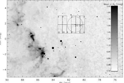
Figure 1.Location of the field with respect to 25 Ori and the Orion belt stars, overlaid on gray-scale contours representing mean 2MASSJ−Kscolors, which trace reddening. Bin size is 0.◦1×0.◦1. Filled circles mark bright stars (V 6.0 mag), with size varying linearly with visual magnitude; the brightest of these are labeled, along with 25 Ori which is placed in a chip gap in the PTF field of view. The footprint for each chip in the field is marked and the chip number is identified; the dead chip (NE of the central four) is omitted. The circle shows the 1◦working radius used by Brice˜no et al. (2007) to define the 25 Ori group.
The figure confirms that the amount of interstellar reddening is apparently uniformly quite low in the 25 Ori field, and we adopt the derived mean extinction value for the cluster from Brice˜no et al. (2007;AV =0.29 mag) as a single representative
value. (In comparison, typical values from the dust maps of Schlegel et al.1998along lines of sight to the sources in the field range from ≈0.3 to 0.6 mag, and mostly <1.0 mag. As estimates of the full line-of-sight extinction through to the edge of the Galaxy, these suggest an upper limit.) Following the extinction laws of Cardelli et al. (1989), and assuming RV =3.1, the adopted value ofAV corresponds to extinctions inR, J, H, andKS of 0.22 mag, 0.082 mag, 0.055 mag, and 0.033 mag, respectively.
2.2. PTF Observations
Data were taken for the Orion project on the majority of the clear nights between 2009 December 1 and 2010 January 15. Weather permitting, the chosen primary field was observed in the R filter as near to continuously as possible, whenever it was higher in the sky than an airmass of 2.0. Exposures were 30 s long, with a cadence varying generally between 70 and 90 s, including readout time and depending on the performance of the telescope control system and guiding control loop (see below).
Since the Orion observing program could not easily be incorporated into the normal PTF robotic scheduling, separate scripts for the telescope and camera control code were adapted from the standard PTF robot code for the purposes of the Orion observations. Each night at the beginning of the Orion field observations, normal PTF operations were manually interrupted to run the Orion observing program. When the field center
sets once again below airmass 2.0, control was automatically returned to the standard PTF robot scheduler and normal PTF operations resumed.
Of the 40 nights dedicated to the Orion project, 14 yielded usable data, the majority of the remainder being either of marginal quality due to clouds or subject to telescope closure because of poor weather. (One night also could not be processed due to an insufficiency of non-Orion exposures to create a flat field for that night, and can in principle be recovered.) A total of 4486 exposures were taken during the run. An average across the chips of≈3460 exposures ran successfully through the pipeline after rejection of those that could be immediately discarded at the outset by visual inspection, and an average of≈2400 of those exposures passed the data reduction pipeline’s automated data quality assessment without flagging. There is some variation in these numbers from chip to chip since each is processed completely independently. Figure 2 shows a histogram of the number of exposures taken on each night, and the fraction of those that passed unflagged for chip 0, which is used as a representative example of all the chips.
In order to minimize the effects of flat-fielding errors for high-precision photometry, it is desirable to minimize image shift on the detector between frames. Since the Palomar 48 inch has no native guiding facility, we developed software to guide on the science images as they came from the telescope, providing feedback to the telescope via offset pointing commands. Off-sets were referenced to a single good quality reference frame taken at the beginning of the run, and telescope pointing up-dates were applied during readout time generally every second frame. On initial pointing of the telescope, offsets of typically
Figure 2.Number of exposures taken per night for the PTF Orion project from 2009 December to 2010 January. Solid black regions indicate the fraction of exposures that remained unflagged after processing by the data reduction pipeline, for chip 0 (similar fractions are seen for the other chips).
corrected within two exposures. With the guiding switched on, the pointing toward the center of the field was stabilized with a root-mean-square (rms) image shift of≈1.0 and≈0.5 pixels in right ascension and declination, respectively, compared to unguided linear tracking drifts of≈0.3 pixel minute−1.
2.3. Ancillary Data
In addition to the PTF data obtained, we also drew on data from several other sources. The photographic US Naval Observatory USNO-B1.0 source catalog (Monet et al.2003) provided a reference data set for initial photometric zero-point correction of the R-band PTF Orion data (Section 3.1). A further catalog of ≈40,000 reference stars from the Centro de Investigaciones de Astronom´ıa–Quasar Equatorial Survey Team (CIDA-QUEST), provided by C. Brice˜no (2009, private communication), allowed for a final more accurate correction to the R-band zero point after differential photometry had been performed (Section 3.2). This catalog had in turn been calibrated against the Landolt system (Landolt 1992) with R magnitudes ranging from 14R19 and measurement errors varying with increasing magnitude from≈0.015 to 0.1 mag. The overall error for the brighter stars (down to R ≈ 17) including systematics is≈0.02–0.03 mag. We also made use of the PPMXL catalog (Roeser et al. 2010) to obtain proper motions for our candidate binary systems. The PPMXL catalog provides a determination of positions and proper motions by combining USNO-B1.0 and Two Micron All-Sky Survey (2MASS) astrometry, and aims to be completed toV ≈20 mag. The 2MASS point-source catalog (Skrutskie et al. 2006) provides all-sky coverage of point sources in the near-infrared J(1.25μm),H(1.65μm), andKs(2.16μm) bandpasses, with magnitude limits of 15.8, 15.1, and 14.3 mag,respectively. PTF Orion source detections were matched against this catalog to provide color information on each source in combination with the PTF OrionR magnitude. The 2MASS catalog includes a “quality” flag for each measurement in each band, which can take various values. In particular, designations from “A” to “F” represent photometric quality in decreasing order (in the case of an “F,” error estimates could not be determined). In certain cases throughout this paper we use these flags to restrict analysis to sources with 2MASS data above a given quality level, as stated in the text.
For certain target objects, anticipating that these young ob-jects might have discernible mid-infrared (MIR) excesses due to circumstellar disks, we also examined theSpitzer Space Tele-scope(Werner et al. 2004) Heritage Archive for both Infrared
Array Camera (IRAC; Fazio et al.2004) and Multiband Imaging Photometer forSpitzer(MIPS; Rieke et al.2004) data, discussed below. We found some IRAC data (at 3.6, 4.5, 5.8, and 8μm), but MIPS data (at 24μm) were more common in our target region. We found MIPS and/or IRAC data for 15 objects, dis-cussed in Sections5.2.5and6. All 15 of the objects were found in at least one of 9 AORKEYs14: 10987776, 26066432, and/ or 26067456 for IRAC, and 10987008, 17052160, 26067712, 26067968, 26069760, and/or 26070016 for MIPS. The images for each object were examined for potential source confusion, and none was found.
For IRAC, we started from the automatically produced mo-saics from the Archive (S18.7 or greater), and performed aper-ture photometry using the IDL15routine aper.pro16on these mo-saics at the designated positions. We used an aperture radius of 3 native pixels (1.2 arcsec pixel−1), a sky annulus of radius 3–7 native pixels, and multiplicative aperture corrections of 1.124, 1.127, 1.143, and 1.234 for the four channels, respectively, as prescribed by the IRAC Instrument Handbook, available on the Spitzer Science Center Web site. The zero points we used to convert between flux density units (Jy) and magnitudes were, respectively, 280.9, 179.7, 115.0, and 64.13 Jy.
For MIPS, we initially obtained the automatically produced mosaics from the Archive (S18.12 for MIPS), and on a case-by-case basis, reprocessed the mosaics if necessary from the basic calibrated data level, to reduce the influence of instrumental artifacts. We also conducted aperture photometry using IDL’s aper.pro on the mosaics (either ours or the Archive’s), using an aperture of 7, an annulus of 7–13, and an aperture correction of 2.05, from the MIPS Instrument Handbook, again available from the SSC Web site. The MIPS-24 zero point we used was 7.14 Jy.
In the ideal case, to determine whether or not there is infrared excess due to a circumstellar disk, we need an estimate of a spectral type so that we can fit a model to the spectral energy distribution (SED) and estimate reddening (AV), and then estimate the degree of infrared excess due to a disk. In the absence of an accurate estimate of spectral type, the degree of IR excess is not well defined. We can instead attempt to estimate the degree of infrared excess by assuming that these sources
14 AORKEYs are the unique eight-digit identifier for the Astronomical
Observation Request, which can be used to retrieve these data from theSpitzer Heritage Archive.
15 http://www.ittvis.com/idl
16 Found in the IDL Astronomy User’s Library,http://idlastro.gsfc.nasa.gov/;
The Astronomical Journal, 142:60 (35pp), 2011 August van Eyken et al. are all truly stars (as opposed to background objects), and then
comparing the longerSpitzerbands to a shorter band. Where possible, even lacking a spectral type estimate, we can use [3.6]−[24] to reasonably reliably indicate disk excess (where the bracket notation denotes the magnitudes at theSpitzerbands), since this range is within the Rayleigh–Jeans tail even for the latest spectral types, giving them colors of zero. Reddening also does not strongly affect this color unlessAV is extreme, in which case the extinction will be high enough to make a source detection unlikely in our PTF data. MIPS-24 data are more widely available in our field than the IRAC bands, however, and 3.6μm data do not always exist. In such cases, the 2MASS Ksband is the most commonly available alternative.Ks−[24]
therefore provides an alternative excess estimate, although it is less reliable since late-type stars (such as many of those in our sample) are not colorless atKs−[24] (Gautier et al.2007), and
the effects of reddening are stronger atKsthan at 3.6μm. For such cases, additional follow-up observations will be needed to refine the estimate of the excess.
3. THE PTF ORION DATA REDUCTION PIPELINE
The initial PTF data reduction pipeline in place at the time the data were taken was geared primarily toward absolute photometry and extensive database operations for handling the vast quantities of data coming from the broader survey. We developed a separate dedicated relative-photometry pipeline, which took over from the standard pipeline at the point where image processing was complete. Here, we describe the two broad steps in the data reduction procedure: obtaining the initial raw photometry, beginning with the standard PTF image processing and the first steps of the Orion pipeline, and the differential photometry process used to obtain the precisions needed for the PTF Orion survey.
3.1. Raw Photometry
The main PTF pipeline image processing consisted of stan-dard bias subtractions, flat fielding, and astrometric solutions. Each chip was reduced separately and in parallel. Floating bi-ases were measured as the median of the overscan regions of the chips and subtracted along with a nightly combined superbias frame; flat fields were created by combining all (non-Orion-project) images taken with the same filter during a night, all the bright pixels first being masked out using SExtractor (Bertin & Arnouts1996), to leave a pure sky flat field. Astrometric infor-mation was added to the FITS image headers using SCAMP (Bertin 2006) to solve for the astrometry. The general PTF pipeline is discussed in more detail in Grillmair et al. (2010) and R. Laher et al. (2011, in preparation).
The Orion pipeline ran separately and took as input the image data from the standard pipeline after the astrometric solutions had been added. Written in IDL, the main steps in the PTF Orion pipeline are as follows.
1. Pixel masking. Masks are initially applied to reject any badly behaved pixels on the detector using an algorithm loosely based on the IRAF17 “ccdmask” procedure (Tody 1986, 1993). Masks are created from images made by dividing a 70 s light-emitting diode (LED18) flat field by a 35 s LED flat field; three independent such divided frames were obtained for each chip. Any pixels with outlier fluxes
17 http://iraf.noao.edu/
18 Light-emitting diode—see Law et al. (2009).
beyond 4σ in at leasttwoof the three frames, or beyond 3σ in all three of the frames were flagged as bad. This approach helps catch excessively variable pixels in addition to nonlinear pixels, while still rejecting cosmic-ray hits. The flagging procedure was then repeated several times after boxcar smoothing of the original image along the readout direction with a selection of bin sizes from 2 to 20 pixels (this removes columns where individual pixels are not statistically bad, but are statistically bad when taken as an aggregate). Pixels lying in small gaps between bad pixels were then also iteratively flagged, with the aim of completely blocking out large regions of bad pixels while minimizing encroachment into good pixel regions. Any source detection with a flagged pixel within its photometry aperture is rejected and does not pass through the pipeline. 2. Raw photometry.Source detection and aperture photome-try are performed using the IDL Astronomy User’s Library implementation of DAOPHOT (Landsman 1993; Stetson 1987), with minor modifications to return more significant figures in the output files and to handle the large num-ber of sources in each CCD frame. Owing to the some-times large offsets of the field on the detector from image to image, source detection is performed separately on ev-ery exposure obtained, with a 4σ detection threshold. A 4 pixel aperture radius provides a reasonable compromise between maximizing the flux enclosed for bright sources and minimizing sky-background noise for faint sources, while also being large enough to prevent significant pho-tometric errors from imperfect centroiding of the aper-tures. This compares to median seeing of 2.5 at FWHM (where 1 pixel ≈1). Inner and outer radii of 10 and 20 pixels, respectively, are chosen for the annulus used for background estimation around the aperture. The de-fault limits for “sharpness” and “roundness” of the detected sources provide a first cut to reject cosmic rays and back-ground galaxy detections.
3. Initial zero-point correction.An initial zero-point correc-tion is applied by matching deteccorrec-tions against the USNO-B1.0 catalog and correcting for the outlier-resistant19mean difference between raw and USNO-B magnitudes for each image from each chip. This places all photometry on an absolute scale, within the accuracy of the USNO-B catalog (∼0.3 mag). Sloan Digital Sky Survey (SDSS) photometry data would provide a more accurate correction, but were not available for the 25 Ori field.
4. Creation of master source list.After filtering out images with poor seeing or high background, a master source list for each chip is created by stepping through each of the 100 images with the highest numbers of source counts, in decreasing order of source counts. For each image, if a source is detected whose sky position cannot be matched with one already found (within a 2 radius, the matching radius used throughout the pipeline), it is added to the master list. On every 20th image, sources with only one detection are pruned from the table, as are any sources with fewer than 10 detections at the end of the process. This ensures that cosmic rays, asteroids, and spurious detections are rejected from the table. Since we are primarily concerned with persistent stellar objects with relatively low-level variability, we accepted the consequent
19 Throughout this text, where an outlier-resistant mean or standard deviation
loss of short transient events that may appear from below the detection limit in return for the significant savings in data storage space in the final output data tables. This does not affect any of the sources that are suitable for planet transit searches.
3.2. Differential Photometry
After the initial raw photometry and preparation of the master source lists, a single data table for each chip is prepared with entries for each source in the lists at each epoch of observation. A second pruning of the table is performed to remove sources if they show very few total detections (fewer than 100) and those detections are sparsely distributed in time (the fraction of successful detections within any 50 consecutive epochs is less than 0.5). This helps remove sources which are due to badly behaved pixels or on the extreme edge of the detection limit, while retaining genuine transients that are only detected for a limited length of time. The source list from each chip is then split into four equal-area quadrants, each treated separately. This provides a first-order accommodation for variations in photometry across the wide field of view which may be caused by thin cloud, variations in point-spread function (PSF) due to the wide-field optics, effects of differential airmass variation, and atmospheric refraction (see Everett & Howell 2001). On average≈2600 sources were detected per chip quadrant for the 25 Ori field.
In a given quadrant, an outlier-resistant mean magnitude is then calculated for each source across all epochs; this creates a reference magnitude list against which to perform the differential photometry. For each observation, the difference is calculated between every source’s measured magnitude and its corresponding reference magnitude. Within each quadrant, the mode of the differences is then calculated and subtracted from the measured magnitudes to provide the differentially corrected magnitudes. The mode is calculated by fitting a Gaussian curve to the peak of the histogram of magnitude differences in the quadrant, and the peak of this Gaussian is taken to represent the best-likelihood estimator of the true fine-scale correction for the zero point of the frame. All stars in a given quadrant are thus used in establishing the differential correction applied for that quadrant.
Using the modal magnitude difference correction in this manner has the advantage of being very robust to outliers and variable stars. It also requires no selection of an ensemble set of stable reference stars, provided that there is a sufficient number of stars in the field and that a sufficient number of those stars are relatively stable. Even in the event that only a small fraction of stars are stable, provided that the total number of stars is large, the mode still represents a reasonable estimate of the differential correction since there is no reason to expect any correlation in intrinsic variability between the stars included in the histogram. Additionally, the modal difference draws information from the full ensemble of stars, providing a natural “weighting” of the differences: stars that have higher photometric uncertainties (i.e., lower fluxes) or that are more variable will contribute a more spread-out Gaussian to the total distribution, adding more to the wings of the histogram, though still peaking around the true magnitude difference; those with lower uncertainties (high fluxes) will contribute a tighter Gaussian to the total and contribute more to the peak of the histogram.
To further improve the statistics, the differential photometry is then repeated after identifying and omitting from the histogram sources which still show an rms variation greater than 4σabove
their mean measurement error, or an rms variation greater than 2% (or more precisely, an rms greater than the quadrature sum of these two values). This entire procedure is iterated until the total number of sources rejected in this way changes by less than 3%.
As a final step, once differential photometry is complete, the real apparent magnitude is set by comparing the median magnitudes of each differentially corrected time series against the list of stable reference stars from the CIDA-QUEST survey, which in turn are calibrated against the Landolt system (see Section2.3). The median of the differences is used to provide a final single zero-point correction for each entire chip.
After processing, the data are automatically checked and any questionable sources, nights, or individual data points are flagged according to a number of criteria. Flags are added for failed DAOPHOT photometry or differential photometry; multiple source detections, USNO-B reference sources, or master-list sources, within the FWHM; high image background, very low zero point, or high variation in background across the image; exceptionally large FWHM; low number of sources across the image; large variations with time in the measured right ascension/declination for an individual source location; saturation; high sigma or skew in individual background annuli for sources; proximity to predicted optical ghosts; and indication of crowding or contamination within the photometry aperture (assessed by finding outlier values for the ratio of flux inside the aperture to that in a thin annulus around the aperture compared to other sources in the field).
4. DATA
The differential photometry pipeline yielded a total of 116,285 individual light curves (including some resulting from false multiple detections on saturated stars). For an initial inves-tigation of the clearly variable stars, a subsample of all the light curves with an outlier-resistant rms variation greater than three times the outlier-resistant mean measurement error for each light curve was selected. This cut alone yielded≈2060 sources. These light curves and their corresponding images were visually inspected to select only those that clearly represented intrinsic photometric variation, rather than crowded sources or image artifacts that had escaped flagging, sources on unmasked bad pixels, or sources whose variability was clearly due to known systematics (see Section4.1). This initial inspection yielded a total of≈530 sources, the difference in number from the first cut being primarily due to the≈4 mmag noise floor at the bright end which was not accounted for, and to biasing toward light curves that were not too sparsely sampled. (For comparison, se-lecting only sources with>1000 of a possible≈2400 unflagged detections, and rms greater than three times the quadrature sum of the mean measurement error and the noise floor, yields≈700 light curves.) Among the light curves selected from the initial inspection, we visually identified 82 eclipsing binaries and 16 likely CTTS light curves. The results presented in this paper are based on these last two groups of light curves.
4.1. Precision and Sensitivity
The Astronomical Journal, 142:60 (35pp), 2011 August van Eyken et al.
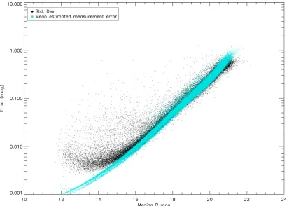
Figure 3.Standard deviation (black points) vs. median magnitude, compared to theoretical photometric errors (cyan; gray in the printed journal), for all unflagged data fromalllight curves obtained with more than 10 good data points. There is a slight overdense band around 0.02–0.03 mag attributable to chip 4, where a known systematic trend affects certain localized regions. See Section4.1.
(A color version of this figure is available in the online journal.)
4 mmag is evident. Approximately 8% of all light curves with more than 10 detections have an rms<1%. The banding in the theoretical errors comes from the different chips and is likely due to small differences in quantum efficiency. Saturation begins to set in around R ≈ 13 mag, where the upturn in the rms appears. The faint-end limit varies depending on the chip, but the turn-over in the number of source detections with increasing faintness begins to set in around R ≈ 19.5 mag, with few detections beyond 20.5 mag.
In addition to intrinsically variable stars, some of the scatter of points above the noise floor at brighter magnitudes in Figure3 is due to systematic trends that appear in small regions of certain chips. After performing differential photometry, it is not unusual to discover common systematic trends in some of the resulting light curves that may be a function of position, color, and/or airmass. An advantage of the “modal differencing” technique employed in the differential photometry (Section3.2) is that, provided the fraction of sources in the ensemble exhibiting a given trend is relatively small, the position of the peak of the difference histogram should be insensitive to the trend. As a result, sources that are not directly affected by the trend will also not be compromised as a result of the differential photometry corrections.
The presence of trends appears to be fairly minimal in the PTF Orion differential photometry, with the exception of one effect that is attributed to known fogging of the detector during the period of the Orion observations, due to slow deposition of oil contaminants from the dry-air system used at the time to prevent condensation on the CCD window (see Law et al.2010). This contributes a slow long-term trend in certain regions of the detector over the length of the observations, with the exception
of the last night, just before which the CCD window had been cleaned. After the cleaning the affected light curves returned to their initial flux level. The trend causes a variation of up to
≈0.2 mag in the worst cases, but is generally easy to recognize, and appears to be confined to relatively small regions on the detector; only a small fraction of the light curves are significantly affected at the level of variability with which we are concerned here. Chip 4 suffered the most from the fogging effect, which leads to a slight overdense band of sources from that chip around 0.02–0.03 mag in Figure3. At this point light curves that clearly show the trend are rejected from our current analysis for simplicity (four probable eclipsing binaries are affected in this way). A number of sources on chip 4 alone also show random noise on the few percent level on the first three nights and the last night of the run, which may be detector noise related. This should be borne in mind with regard to results from that chip.
There are some suggestions of other small trends, possibly color related, but no detrending of the data has been attempted at this stage, and none of these effects are accounted for in Figure3. Nonetheless, the figure shows that the majority of the data are well behaved down to the 4 mmag noise floor without any detrending.
4.2. Absolute Photometric Accuracy
of the CIDA-QUEST list (including systematics), we therefore conservatively estimate the zero points of the individual light curves to be accurate to≈3%–5% for chips 0–4 and 6–10.
The area covered by chips 5 and 11 in the Orion field had no coverage in the reference star set, and therefore no direct secondary zero-point correction could be determined. Instead, a correction was made based on the weighted mean of the corrections from the other chips, excluding only chip 4, owing to more significant fogging-trend systematics on that chip which give rise to a distinctly bimodal, non-Gaussian distribution in the zero-point histogram for that chip. The mean of the secondary zero-point corrections for the remaining chips was 0.159 mag, with a standard deviation of 0.044 mag. Adding this whole-chip zero-point uncertainty in quadrature with the typical uncertainty for the individual light curves discussed above, and a 0.03 mag error for the CIDA-QUEST list, yields an absolute accuracy estimate of 0.069 mag for the light curves on chips 5 and 11.
Marginal color-dependent trends are seen in the magnitude residuals against the CIDA-QUEST references (as a function ofR−I), but they are below the level of the random scatter in the residuals, implying that errors due to mismatch between the PTF and CIDA-QUEST filters are negligible at our accuracy level. Since the error estimates for the zero points are based on the scatter in the residuals about the mean, rather than the error in the mean itself, any systematic errors in zero point should be included in the accuracy estimate.
5. ECLIPSING BINARY SYSTEMS
Among the most easily identified of the light curves are the eclipsing binaries. In this section, we present those found in this initial investigation. Section 5.1 presents an overview of the data; an analysis is presented in Section5.2, where we identify candidate young binaries, and Section5.3, where we identify some additional low-mass systems. In Section5.4, we summarize and discuss the specific notewor-thy sources.
5.1. Eclipsing Binary Results
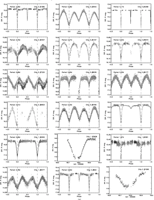
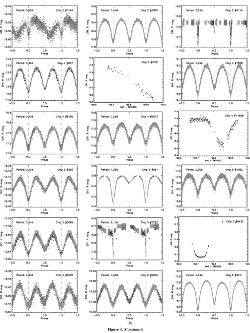
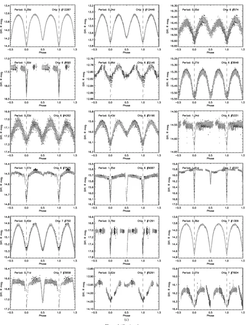
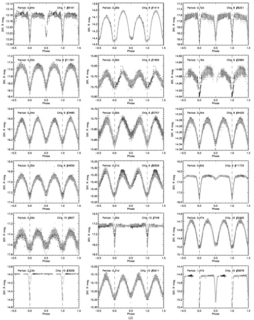
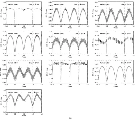
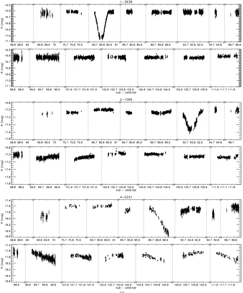
We identified a total of 82 clear eclipsing binaries in the PTF Orion data, for which period-folded light curves are presented in Figure4. These were identified by visual inspection of our short list of strongly varying light curves, most eclipsing binary light curve types displaying distinctive characteristic shapes. Light curves that were sinusoidal in appearance were rejected due to the ambiguity in interpretation of their nature. Among the binaries, three were found to have been previously identified as candidate variable stars by Kraus et al. (2007) in the MOTESS-GNAT survey (sources 0-9653, 5-12287, and 5-12446). In those cases where a period could not be determined, either because too few eclipses were detected or because the data did not show a regular period, the data covering only the best-captured eclipse are instead plotted against time to show the eclipse shape. The complete light curves for the five such targets are shown in addition in Figure5.
Table 1 lists the basic properties of the eclipsing binary systems: the assigned PTF Orion survey ID,N-n, consisting of the chip number,N, on which the source was detected, followed by a running sequence number,n; the mean measured J2000 coordinates over the whole observing run (accurate to≈1 inch); the corresponding 2MASS ID where a match was obtained (Skrutskie et al.2006); the 2MASSJ,H, andKs magnitudes; classification as “close” (C) or “detached” (D) (see below); the
period,P, in days;T0, the heliocentric Julian date for the epoch of the primary eclipse; the estimated distance to the system; the median-measuredRmagnitude; andΔR, the approximate peak-to-peak magnitude range of the measured light curve. Specific sources discussed in the text are broken out at the beginning of the table. The newly measured properties in the table are obtained as described below.
Classification.The 82 systems are categorized into one of two broad classifications: “close” (“C”), of which we find 45, and “detached” (“D”), of which we find 37. For the purposes of this paper, “close” systems are defined as those for which there is no apparent distinction between in- and out-of-eclipse regions in the light curve, i.e., where there is no clear discontinuity in the slope of the curve. These should represent, for the most part, contact and overcontact binary systems. Those for which such a distinctionisapparent are considered “detached,” though this category can also include semi-detached and near-contact systems. In some cases semi-detached or near-contact systems may also fall into the “close” category instead, depending on the exact nature of the light curve. We have not attempted to further sub-classify the binary systems to avoid ambiguities that are better addressed with full light curve modeling.
Orbital parameters.Orbital periods,P, are obtained by cal-culating the Plavchan periodogram of the light curve (Plavchan et al.2008), using a stand-alone version of the NASA/IPAC/ NExScI Star and Exoplanet Database periodogram service.20 The light curve is folded on the period corresponding to the highest peak in the periodogram, and visually inspected to con-firm the period is reasonable. If not, the next highest peaks are investigated until a plausible folding is found. The error in the period is estimated from the width of a Gaussian fit to the cor-responding peak. In cases where the shape of the peak was such that a good Gaussian fit could not be made, the approximate peak was estimated by hand, and an appropriately large error assigned.
The time of mid-eclipse,T0, for the systems is measured by fitting a symmetrical inverted trapezium to the deepest and best-sampled minimum of each light curve and calculating the center time of the fitted trapezium. This fit also yields the formal errors for the eclipse center time.
Distance. W UMa systems display a relatively well-established empirical period–color–luminosity relationship re-sulting from their approximately uniform temperature common envelope:Kepler’s law constrains the orbital radius as a function of period, and the orbital radius in turn constrains the radiating surface area and, hence, the luminosity and absolute magnitude of the system (Rucinski2004). They therefore can be used as distance estimators. Eker et al. (2009) provided an updated cali-bration of the relationship based on 2MASS (J−HandH−Ks)
colors; we use this relationship to estimate the distances for the “close” binaries in the table where the detections have 2MASS counterparts, on the assumption that the vast majority are W UMa systems.
Bilir et al. (2008) provided a similar empirical relationship between 2MASS colors and absolute magnitude for main-sequence-detached binaries, analogous to the color–luminosity relationship for single main-sequence stars. We apply this relationship to the “detached” binaries in the table, on the assumption of dwarf star status.
Errors in the derived distances are estimated by standard propagation of the 2MASS photometric errors through the
20 http://nsted.ipac.caltech.edu/periodogram/cgi-bin/
The Astronomical Journal, 142:60 (35pp), 2011 August van Eyken et al.
[image:9.612.54.561.45.702.2](a)
(b)
The Astronomical Journal, 142:60 (35pp), 2011 August van Eyken et al.
[image:11.612.54.561.48.718.2](c)
(d)
The Astronomical Journal, 142:60 (35pp), 2011 August van Eyken et al.
[image:13.612.76.540.52.469.2](e) Figure 4.(Continued)
respective empirical relationships. The errors in the coefficients in the relationships are neglected, but the reported standard deviations about the relationships (0.26 mag and 0.49 mag for the W UMa and detached-system calibrations, respectively) are added in quadrature to account for astrophysical effects that are not included in the relationships. In both cases, the effects of reddening are also neglected: for our assumed value ofAVat the distance of 25 Ori, using the extinction laws of Cardelli et al. (1989) gives reddening values ofE(J−H)=0.027 mag and E(H−K)=0.022 mag, which in most cases are comparable to or less than the photometric measurement errors. Neglecting reddening does lead to a small systematic underestimation of the distances, generally by of order one half the measurement error in most cases for our assumed meanAV, and always less than the full size of the error, but it is simpler than attempting to realistically estimate the reddening for each individual source.
We note that these distance relationships are likely to be in-accurate at PMS ages. Low-mass stars (<1.5M) younger than 10 Myr will still be on PMS tracks and can be expected to be brighter than predicted (albeit the close companions in our sam-ple may complicate the evolutionary picture). The agreement
between the list of young candidates from the color–magnitude diagram and the list from the distance estimates, however, pro-vides some suggestion that the estimates are still meaningful in these cases (see Sections5.2.1and5.2.2). Some systems also represent extrapolations beyond the formal calibrated limits of the relationships provided by Eker et al. (2009) and Bilir et al. (2008), particularly for the detached systems at apparent types later than mid-K. The distances provided in the table therefore are only intended as a guideline and should be treated with appropriate caution.
(a)
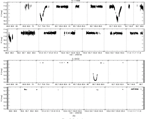
Figure 5.Full unfolded light curves for those sources for which a period could not be uniquely determined due to an insufficient number of eclipse detections or because the data did not exhibit a regular period. 5-6432 (b, bottom panel) shows sparse coverage because most of the data is saturated; the light curve drops below the saturation threshold during the eclipse, however.
5.2. Identifying Young Binaries
We identify young binary candidates in our sample with a color–magnitude selection, and then follow several approaches to check for consistency, detailed below. We find nine candidates that are worthy of follow-up (see beginning of Table1).
5.2.1. Color–Magnitude Selection
The Astronomical Journal, 142:60 (35pp), 2011 August van Eyken et al.
[image:15.612.64.550.58.456.2](b) Figure 5.(Continued)
flags worse than “C” or error bars>0.1 mag—see Section2.3). Isochrones are overplotted which are based on the Siess et al. (2000) models. These are tuned to fit the Pleiades main sequence at 100 Myr (Guieu et al. 2010; Stauffer et al. 2007; Jeffries et al. 2007), and then converted to R versus R −Ks using
polynomial fits to young star colors (Kenyon & Hartmann1995). The blue triangles mark the locations of previously identified (single) WTTS stars identified by Brice˜no et al. (2007) which are also found in our data and in the 2MASS catalog. They lie along the 10 Myr isochrone, in good agreement with the 10 Myr age determined by Brice˜no et al. (2007) also using Siess et al. isochrones, and supporting our placement of the isochrones in the diagram.
The uncertainties of magnitudes and colors are dominated by the amplitude of the physical photometric variability. As a result the error bars in Figure6are assigned to represent the overall variability of the light curves (half the peak-to-peak amplitude). In the absence of multi-epoch 2MASS measurements, we assume the variability inKsto be the same as that in the PTFR measurements for the purposes of the error bars, and since the RandKsare not contemporaneous, we assume the errors to be independent. We treat the WTTS sources in the same way to allow for their variability as well.
Those systems lying below the marked main sequence are taken to be unassociated with the 25 Ori/OB1a association. Those falling above the main sequence (the PMS region for the assumed 25 Ori distance and reddening) are highlighted with star symbols, and identified as candidate young systems. This criterion yields nine systems: 0-7220, 2-1066, 2-1144, 4-5331, 5-12446, 7-5291, 7-7604, 10-10597, and 11-5402 (see Table1). For comparison, we ran a Besan¸con Galactic model simulation for the PTF Orion field using the default model parameters21 (Robin et al.2003). This allows us to estimate how many field stars might be expected to lie in the PMS region. Scaling the fraction of sources found to lie above the 330 pc main sequence in the simulation to the size of our binary sample yields≈2–5 expected field sources, depending on the exact location of the main-sequence cut.
There is an ambiguity with regard to binary systems on the color–magnitude diagram in that the mass ratios of the systems are unknown. For systems with a small mass ratio, one star dominates the luminosity, and hence the system’s location on the diagram would fall as expected for a single star of the same type and color (diverging evolutionary effects due to
Astronomical
J
ournal
,
142:60
(35pp),
2011
August
van
Eyken
e
t
a
[image:16.612.43.754.114.518.2]l.
Table 1
New Eclipsing Binaries from the PTF Orion Data
2MASS
ID R.A. Decl. 2MASS/USNOB1.0 J H Ks Class. P T0 Distance Rmedn ΔR
(deg) (deg) (mag) (mag) (mag) (days) (HJD-2455000) (pc) (mag) (mag)
Pre-main-sequence low-mass binary candidates
0-7220 80.26648 2.67426 J05210397+0240275 12.69±0.02 12.06±0.02 11.89±0.02 D 0.679631±0.001025 205.83808±0.00025 349 ±83 14.58 0.06 2-1066a 81.49801 1.96661 J05255953+0157593 13.64±0.03 13.04±0.03 12.76±0.03 D . . . 192.77787±0.00050 428 ±109 17.06 0.58 2-1144 81.45159 1.97448 J05254838+0158276 13.09±0.03 12.43±0.03 12.20±0.03 D 0.554431±0.001839 201.70360±0.00075 337 ±83 16.53 0.14 4-5331b 82.40622 2.35695 J05293750+0221251 14.36±0.04 13.60±0.04 13.17±0.04 D . . . 189.94145±1.00000 270 ±72 17.75 0.87 7-7604c 80.77483 1.64755 J05230596+0138511 13.09±0.03 12.39±0.02 12.18±0.03 D 2.071092±0.009377 211.69810±0.00158 322 ±78 16.18 0.23 11-5402d 83.18037 1.31577 J05324332+0118566 13.44±0.03 12.81±0.03 12.55±0.03 D 5.505740±0.355271 199.83101±0.00032 391 ±98 15.79 0.29
Other low-mass candidates
2-822 81.59643 1.93894 J05262316+0156196 15.26±0.07 14.67±0.07 14.29±0.08 D 0.920431±0.000166 180.83174±0.00012 694 ±245 16.82 0.89 5-5767 83.10952 2.38606 J05322632+0223097 15.16±0.06 14.58±0.06 14.32±0.08 D 2.104862±0.002494 211.71483±0.00044 946 ±326 16.73 0.33
Pre-main-sequence close-binary candidates
5-12446o 83.34683 2.97482 J05332318+0258281 11.99±0.03 11.47±0.02 11.34±0.03 C 0.236633±0.000017 204.65544±0.00003 317 ±41 13.46 0.39 7-5291e 80.80171 1.35431 J05231240+0121151 12.13±0.02 11.44±0.02 11.31±0.02 C 3.623108±0.023858 192.86419±0.00265 1442±183 13.95 0.11 10-10597 82.53469 1.81344 J05300832+0148489 11.77±0.03 11.27±0.03 11.13±0.02 C 0.299531±0.000050 192.72915±0.00008 348 ±45 12.96 0.18
Other binaries of interest
0-3542 80.00204 2.25436 J05200049+0215159 14.27±0.03 13.74±0.02 13.51±0.04 C 0.284425±0.000077 199.77639±0.00023 934 ±122 15.62 0.28 0-9653o 80.29957 2.93869 J05211191+0256189 14.70±0.05 14.18±0.04 13.88±0.06 C 0.910619±0.001313 202.84000±0.10000 2273±339 16.23 0.29 9-2980l 81.86439 0.98081 J05272748+0058506 14.39±0.04 14.12±0.04 14.11±0.07 D 1.190701±0.003662 175.79416±0.00062 2923±900 14.87 0.07 11-7037 82.87870 1.50007 J05313088+0130004 15.01±0.05 14.50±0.07 14.25±0.09 C 0.306948±0.000228 199.74559±0.00116 1395±235 16.09 0.13 11-8774f 83.32166 1.68053 J05331720+0140498 13.23±0.03 12.62±0.03 12.47±0.03 C 0.215651±0.000007 180.94621±0.00004 450 ±60 14.83 0.78
Other binaries
0-1580 79.94125 2.02664 J05194592+0201361 14.35±0.04 13.91±0.04 13.78±0.05 D 2.061758±0.001051 198.80653±0.00012 1334±376 15.56 0.52 0-4268 80.46153 2.33903 J05215079+0220205 13.03±0.03 12.67±0.02 12.66±0.03 D 5.167944±0.176421 202.79638±0.00003 1233±307 13.90 0.70 0-4407 80.17316 2.35519 J05204154+0221186 14.60±0.03 14.07±0.04 13.97±0.07 D 0.701540±0.001087 189.75110±0.00039 1296±389 16.07 0.15 0-5197 80.45244 2.44664 J05214859+0226480 16.20±0.13 15.42±0.11 15.60±0.25 C 0.273236±0.000064 198.80522±0.00047 2006±627 17.24 0.80 0-5673 80.06399 2.50293 J05201536+0230104 14.91±0.05 14.39±0.04 14.34±0.08 D 0.543151±0.000185 175.83572±0.00037 1786±602 15.93 0.19
0-8036g 80.03662 2.76290 0927-0078105 . . . . . . . . . D 0.597359±0.000604 204.70458±0.00048 . . . 18.09 0.75
0-8177 80.28231 2.77769 J05210774+0246397 15.98±0.08 15.82±0.14 >15.21 C 0.304414±0.000214 204.74716±0.00047 . . . 17.11 0.25 0-9790 80.42457 2.95301 J05214195+0257109 15.96±0.10 15.77±0.14 15.49±0.23 C 0.326311±0.000147 199.72763±0.00036 3842±1112 17.12 0.43 1-1223 80.94578 2.00642 J05234700+0200225 15.26±0.05 14.80±0.07 14.87±0.13 D 1.252181±0.000334 192.80870±0.00012 3488±1528 15.91 1.59 1-2659 80.80171 2.18552 J05231240+0211079 15.99±0.11 15.90±0.19 15.12±0.16 D 0.960161±0.002785 189.89204±0.00025 1045±585 16.67 0.59 1-3638a 81.08221 2.31406 J05241975+0218507 15.68±0.07 15.46±0.12 15.43±0.20 D . . . 180.78801±0.00028 5650±3628 16.63 0.43
The
Astronomical
J
ournal
,
142:60
(35pp),
2011
August
van
Eyken
e
t
a
[image:17.612.48.736.121.510.2]l.
Table 1 (Continued)
2MASS
ID R.A. Decl. 2MASS/USNOB1.0 J H Ks Class. P T0 Distance Rmedn ΔR
(deg) (deg) (mag) (mag) (mag) (days) (HJD-2455000) (pc) (mag) (mag)
1-4581j 80.66826 2.43163 J05224038+0225541 14.48±0.03 14.11±0.04 14.12±0.07 D 1.870680±0.002107 175.74000±0.10000 2489±760 15.44 0.17 1-6477 80.54039 2.66092 J05220972+0239392 13.30±0.03 13.06±0.03 12.98±0.03 C 0.779850±0.001626 202.77152±0.00119 2159±284 14.24 0.05 2-1985 81.48699 2.06813 J05255688+0204050 15.27±0.05 15.12±0.10 14.91±0.14 C 0.303446±0.000047 202.78324±0.00015 3083±630 16.47 0.55 2-4114 81.23841 2.30490 J05245720+0218173 16.02±0.09 15.88±0.18 >15.29 D 3.519536±0.005422 189.81694±0.00034 . . . 16.93 0.45 4-827 82.72646 1.93051 J05305436+0155497 12.78±0.03 12.40±0.03 12.29±0.03 C 0.322230±0.000100 199.75955±0.00006 738±96 13.65 0.35 4-7558 82.67281 2.56394 J05304150+0233503 15.19±0.06 14.83±0.07 14.66±0.10 C 0.258346±0.000040 204.70188±0.00013 1904±337 16.31 0.42 4-8796 82.58078 2.67704 J05301942+0240378 16.14±0.12 16.13±0.23 >15.51 C 0.397136±0.000170 198.83439±0.00056 . . . 17.04 0.41 4-9573 82.76732 2.74706 J05310413+0244486 16.01±0.11 15.55±0.16 14.91±0.14 C 0.264623±0.000081 201.84733±0.00021 1596±424 17.22 0.48
4-11668h 82.35476 2.93170 J05292516+0255538 16.21±0.12 15.76±0.15 >15.63 D . . . 175.75243±0.00069 . . . 17.64 0.75
5-295 83.34093 1.88633 J05332181+0153105 15.68±0.09 >15.32 >15.66 C 0.422437±0.000242 201.85629±0.00035 . . . 16.20 0.20 5-961 82.91029 1.95100 J05313843+0157027 12.91±0.02 12.65±0.03 12.62±0.03 D 1.331246±0.000334 169.97516±0.00027 1417±353 13.87 0.48
5-4382 83.05060 2.26285 0922-0084153 . . . . . . . . . C 0.303254±0.000128 205.85421±0.00060 . . . 17.88 0.68
5-5669 83.21871 2.37652 J05325252+0222357 12.42±0.02 11.99±0.03 11.90±0.03 C 0.510305±0.000534 189.76562±0.00054 772±99 13.61 0.05 5-6432a 82.90660 2.44429 J05313758+0226397 11.67±0.03 11.32±0.02 11.24±0.02 D . . . 189.72730±0.00004 554±134 12.67 0.49 5-8209 83.10664 2.60591 J05322562+0236214 14.88±0.05 14.39±0.05 14.24±0.08 C 0.295733±0.000223 189.87958±0.00071 1441±228 16.50 0.14 5-8640i 83.26033 2.64550 J05330249+0238437 14.50±0.04 14.17±0.05 14.19±0.08 C 0.329931±0.000178 189.89227±0.00017 2001±307 15.56 0.10 5-9211 83.39732 2.69212 J05333535+0241314 14.41±0.04 13.91±0.04 13.80±0.06 C 0.243963±0.000012 199.86100±0.00009 1052±151 15.94 0.96 5-12287o 83.34737 2.96147 J05332334+0257401 12.45±0.03 11.99±0.03 11.86±0.03 C 0.287096±0.000012 204.75612±0.00002 500±64 13.79 0.75 6-574 80.02016 0.77828 J05200487+0046426 15.50±0.05 15.01±0.07 14.88±0.13 C 0.549560±0.000737 180.79434±0.00120 2893±539 16.48 0.20 6-690j 79.97470 0.79530 J05195397+0047438 16.03±0.10 15.34±0.09 15.39±0.18 D 1.499817±0.000954 180.91794±0.00043 2672±1611 17.37 0.94 6-2146c,m 79.97923 0.98111 J05195505+0058522 12.06±0.03 11.85±0.02 11.78±0.02 C 0.964920±0.002042 199.85344±0.00165 1454±186 12.80 0.05 6-3648 80.38690 1.16913 J05213285+0110085 14.58±0.03 14.15±0.04 14.16±0.07 C 0.270660±0.000069 201.76570±0.00024 1507±218 15.40 0.20 6-4262 80.51065 1.24251 J05220252+0114330 16.10±0.10 15.91±0.15 15.46±0.20 C 0.328103±0.000301 180.90403±0.00088 3579±1002 17.13 0.28 6-5196 80.46700 1.35628 J05215210+0121224 15.33±0.05 15.04±0.09 15.13±0.17 C 0.425248±0.000221 201.82021±0.00044 3887±832 15.97 0.22 6-5331k 80.29305 1.37240 J05211032+0122202 13.40±0.03 12.96±0.03 12.85±0.03 D 1.242543±0.003772 201.69228±0.00063 930±233 14.55 0.08 6-7525 80.29326 1.63339 J05211040+0138003 13.77±0.03 13.53±0.04 13.47±0.04 D 1.569462±0.000698 189.87010±0.00016 2023±530 14.50 0.28 6-9087 80.50852 1.82028 J05220211+0149141 14.28±0.03 13.72±0.03 13.56±0.05 D 1.351641±0.000382 180.74149±0.00018 894±242 15.73 0.43 7-337 80.77330 0.74753 J05230561+0044515 14.34±0.03 13.63±0.04 13.57±0.04 D 1.811381±0.000233 180.90122±0.00009 844±224 15.84 0.91 7-750 80.95319 0.80217 J05234877+0048078 14.41±0.03 14.25±0.04 14.07±0.06 C 0.402915±0.000064 199.66972±0.00022 2467±351 15.04 0.38 7-1291 80.72298 0.87163 J05225353+0052179 15.99±0.09 >15.53 >15.26 D 3.790587±0.023490 180.75767±0.00068 . . . 17.03 0.65 7-1309 80.92900 0.87349 J05234296+0052244 12.96±0.03 12.67±0.03 12.55±0.03 C 0.363835±0.000015 185.84963±0.00006 1000±131 13.98 0.83 7-3958 80.92392 1.19610 J05234174+0111454 15.45±0.07 15.07±0.09 14.67±0.11 D 0.706710±0.000315 205.73030±0.00040 1193±497 16.67 0.45 7-8191 81.06074 1.71670 J05241461+0143004 12.16±0.02 11.78±0.02 11.76±0.03 D 0.937275±0.000397 199.87813±0.00017 776±188 13.16 0.09 8-1414 81.67115 0.83737 J05264107+0050147 13.30±0.03 12.88±0.03 12.81±0.03 C 0.281382±0.000020 199.83044±0.00007 820±107 14.19 0.43 8-8251 81.17790 1.53097 J05244268+0131514 15.99±0.12 15.80±0.17 >14.98 D 0.718476±0.000247 211.64936±0.00042 . . . 17.66 0.89
Astronomical
J
ournal
,
142:60
(35pp),
2011
August
van
Eyken
e
t
a
[image:18.612.45.733.80.331.2]l.
Table 1 (Continued)
2MASS
ID R.A. Decl. 2MASS/USNOB1.0 J H Ks Class. P T0 Distance Rmedn ΔR
(deg) (deg) (mag) (mag) (mag) (days) (HJD-2455000) (pc) (mag) (mag)
8-11361 81.57440 1.82366 0918-0060816 . . . . . . . . . C 0.318375±0.000106 180.84402±0.00037 . . . 17.65 0.75
9-1695 82.19286 0.85685 J05284629+0051248 15.15±0.04 14.96±0.07 14.75±0.12 C 0.594296±0.001069 175.76614±0.00116 4098±747 15.71 0.08 9-3480 81.96793 1.02633 J05275232+0101345 15.14±0.05 14.83±0.08 14.88±0.14 C 0.342832±0.000113 204.68358±0.00041 2921±557 16.11 0.23 9-3757i 82.15440 1.05077 J05283707+0103024 15.11±0.05 14.83±0.07 14.74±0.11 C 0.585259±0.000765 201.80116±0.00075 3775±655 15.80 0.13 9-4426 81.81013 1.11631 J05271446+0106585 13.22±0.03 12.82±0.02 12.69±0.03 C 0.239152±0.000056 201.86540±0.00024 698 ±91 14.28 0.10 9-4659 81.86969 1.14085 J05272875+0108267 15.92±0.09 15.50±0.13 15.49±0.22 C 0.297846±0.000110 180.84125±0.00034 3024±833 17.00 0.42 9-6659 82.18806 1.33594 J05284514+0120089 14.33±0.03 13.93±0.05 13.86±0.05 C 0.310999±0.000134 204.68321±0.00031 1458±207 15.40 0.19 9-11733 82.00983 1.80036 J05280235+0148015 15.93±0.10 15.80±0.18 >16.30 D 0.602753±0.000100 192.72042±0.00007 . . . 16.75 1.06 10-607 82.46420 0.77599 J05295140+0046337 16.29±0.14 16.12±0.19 >15.84 C 0.289616±0.000200 189.72307±0.00075 . . . 17.48 0.38 10-748j 82.52387 0.79020 J05300573+0047249 14.87±0.04 14.24±0.04 14.10±0.07 D 1.261511±0.001564 192.67356±0.00200 1051±337 17.11 0.92 10-2406 82.78685 0.96683 J05310883+0058008 13.52±0.03 13.15±0.03 13.03±0.04 C 0.468237±0.000143 199.83276±0.00016 1313±178 14.77 0.33 10-3009j 82.49377 1.03404 J05295852+0102022 13.13±0.03 12.89±0.03 12.83±0.03 D 2.234000±0.006000 202.82948±0.00011 1504±370 13.99 0.63 10-5611 82.57626 1.31356 J05301832+0118484 14.23±0.04 13.89±0.04 13.77±0.06 C 0.308967±0.000117 180.87753±0.00034 1484±211 15.17 0.14 10-5878 82.81800 1.34175 J05311632+0120299 13.63±0.03 13.26±0.04 13.17±0.04 D 1.466659±0.000361 199.66223±0.00012 1294±339 14.64 0.64 10-7989 82.71804 1.55714 J05305236+0133253 14.03±0.04 13.78±0.04 13.61±0.06 D 3.690487±0.008470 204.88043±0.00031 1611±458 14.64 1.26 11-1051j 82.94454 0.82398 J05314668+0049260 15.91±0.10 15.62±0.12 15.57±0.23 C 0.372703±0.000221 201.79040±0.00050 4185±1216 16.68 0.27 11-3313 83.03217 1.07005 J05320774+0104117 14.06±0.03 13.62±0.03 13.55±0.04 C 0.281535±0.000019 180.87347±0.00006 1128±152 15.33 0.70
11-3778 83.06084 1.12772 0911-0062767 . . . . . . . . . C 0.227754±0.000108 180.90388±0.00060 . . . 18.40 0.91
11-7429 83.03414 1.54127 J05320820+0132287 12.56±0.03 12.30±0.03 12.21±0.03 D 2.034245±0.002301 211.73886±0.00010 1014±252 13.38 0.32 11-10141 83.42733 1.82439 J05334253+0149276 14.25±0.04 13.96±0.03 13.96±0.06 C 0.456071±0.000184 201.79630±0.00022 2319±327 14.95 0.19
Notes.A description of the columns is given in Section5.1. Corresponding light curves are shown in Figures4and5. Distance estimates are omitted in cases where 2MASS magnitudes reported are limits only. Where possible the matched 2MASS identifier is given based on the J2000 source coordinates; in cases where no 2MASS match was found, the corresponding USNO-B1.0 match running-number-based ID is given instead, with the format “NNNN-NNNNNNNN” (with no preceding “J”). The full 2MASS identifier has the format “2MASS JHHMMSSss+DDMMSSs,” where HH, MM, and SSss represent hours, minutes, and seconds of right ascension, respectively; and DD, MM, and SSs represent degrees, minutes, and seconds of declination, respectively. The lower case “s” represents digits to the right of the decimal point. Full PTF survey catalog IDs can be constructed based on these coordinates, using the format “PTF1 JHHMMSS.ss+DDMMSS.s.” Since precision astrometry was not the primary goal of the PTF Orion project, it is preferable to use 2MASS/USNO-B1.0 coordinates for this purpose rather than our PTF Orion measured coordinates.
aOnly one eclipse obtained—period indeterminate.
bPartial coverage of only one (presumed) eclipse obtained—period indeterminate,T
0not well constrained. cT
0not well determined due to incomplete coverage of eclipse. Measurement error may be unreliable. dOnly one (very good) eclipse observed; period based on out-of-eclipse variation.
eUnusual light curve, possible semi-detached system. Listed distance is assuming a contact binary, but using a detached-system distance estimate yields a distance of 268±64 pc—see Section5.4.3.
fVery short period W UMa system—see Section5.4.4.
gUsed center of secondary eclipse forT
0, owing to poor coverage of primary. hThree clear eclipses, but unable to find coherent period—possible triple system?
iNearby second source in USNO-B; chance of slight contamination.
jSecondary eclipse not evident, or primary and secondary eclipses indistinguishable—possible factor of two ambiguity inP.
kOnly two eclipses obtained—period ambiguous.
lApparent pulsating binary—short-period oscillations seen, with∼1/2 hr period. See Section5.4.4.
mSomewhat distorted light curve shape—may actually represent stellar pulsations rather than a binary system (D. Bradstreet 2010, private communication).
nSee Section4.2for a discussion of zero-point accuracy.
oIdentified as a candidate variable star by Kraus et al. (2007).