A Model-Free Control Algorithm Based on the Sliding Mode Control Method with Applications to Unmanned Aircraft Systems

Rochester Institute of Technology

RIT Scholar Works

Theses

4-17-2019

A Model-Free Control Algorithm Based on the

Sliding Mode Control Method with Applications

to Unmanned Aircraft Systems

Adarsh Raj Kadungoth Sreeraj

[email protected]

Follow this and additional works at:https://scholarworks.rit.edu/theses

This Thesis is brought to you for free and open access by RIT Scholar Works. It has been accepted for inclusion in Theses by an authorized administrator of RIT Scholar Works. For more information, please [email protected].

Recommended Citation

1

R.I.T

A Model-Free Control Algorithm Based on the Sliding

Mode Control Method with Applications to

Unmanned Aircraft Systems

By: Adarsh Raj Kadungoth Sreeraj

A Thesis Submitted in Partial Fulfillment of the Requirements for the

Degree of Master of Science in Mechanical Engineering

Department of Mechanical Engineering

Kate Gleason College of Engineering

ROCHESTER INSTITUTE OF TECHNOLOGY

Rochester, NY

2

A Model-Free Control Algorithm Based on the Sliding

Mode Control Method with Applications to

Unmanned Aircraft Systems

By: Adarsh Raj Kadungoth Sreeraj

A Thesis Submitted in Partial Fulfillment of the Requirements for the Degree of

Master of Science in Mechanical Engineering

Department of Mechanical Engineering

Kate Gleason College of Engineering

Rochester Institute of Technology

Approved By:

Dr. Agamemnon Crassidis

Department of Mechanical Engineering

Dr. Amitabha Ghosh

Department of Mechanical Engineering

Dr. Mark Kempski

Thesis Committee Member

Department of Mechanical Engineering

Dr. Jason Kolodziej

Thesis Committee Member

Department of Mechanical Engineering

Dr. Daniel Kaputa

Thesis Committee Member

3

ABSTRACT

4

Table of Contents

ABSTRACT ... 3

LIST OF FIGURES ... 6

LIST OF TABLES ... 9

NOMENCLATURE ... 10

1. INTRODUCTION ... 11

2. LITERATURE REVIEW ... 13

2.1 Generic SMC Schemes... 13

2.2 Model–Free Sliding Model Control Schemes ... 16

2.3 Sliding Mode Control for Underactuated System ... 20

2.4 Sliding Mode Control for Unmanned Aircraft Systems ... 21

3. MODEL FREE SMC ALGORITHM ... 25

3.1 Lyapunov Stability Theory ... 25

3.1.1 Autonomous and Non-Autonomous Systems ... 25

3.1.2 Equilibrium Points ... 26

3.1.3 Concepts of Stability ... 26

3.1.4 Lyapunov’s Direct Method ... 27

3.2 Model Free Sliding Mode Control Scheme... 28

3.2.1 Square and Non-square MIMO Systems ... 28

3.2.2 System Description for Squared MIMO Systems ... 29

3.2.3 Second Order MIMO System Control Law ... 30

3.2.4 Asymptotic Stability of the Control Law ... 31

3.2.5 The Switching Gain ... 32

3.2.6 The Boundary Layer ... 33

3.3 Second Order System Illustration ... 33

4. METHODOLOGY ... 39

5. SIMULATION STUDY ... 40

5.1 Quadcopter Plant Model... 40

5.1.1 Plant Model States ... 40

5

5.1.3 Plant Model Equations... 44

5.1.4 Thrust Equations ... 46

5.1.5 Motor Dynamics ... 48

5.2 Control Approach for Quadcopter... 49

5.2.1 Actuator Dynamics ... 51

5.3 Basic Quadcopter Simulation ... 52

5.4 Model Sampling Rate ... 56

5.5 State Estimation... 57

5.5.1 Complimentary Filter ... 59

5.6 Sensor Modeling ... 61

5.7 NED to Body Reference Frame ... 63

5.8 Hardware Simulations ... 65

5.8.1 Gimbal Simulation ... 65

5.8.3 Full Model Simulation ... 70

6. HARDWARE TESTING ... 76

6.1 Hardware Description ... 76

6.2 Gimbal Hardware Testing & Results ... 78

6.2.1 Gimbal Hardware Testing with Different λ ... 83

7. CONCLUSIONS ... 88

8. FUTURE WORK ... 90

6

LIST OF FIGURES

Figure 1: Concepts of Stability [1] ... 27

Figure 2: Position Tracking of (a) X1, (b) X2 ... 35

Figure 3: Position Tracking Error of (1) X1, (b) X2 ... 36

Figure 4: Velocity Tracking of (a) X1, (b) X2 ... 36

Figure 5: Velocity Tracking Error of (a) X1, (b) X2 ... 36

Figure 6: Acceleration Tracking of (a) X1, (b) X2 ... 37

Figure 7: Acceleration Tracking Error of (a) X1, (b) X2 ... 37

Figure 8: Controller Effort (a) U1, (b) U2 ... 38

Figure 9: Sliding Condition Constraint ... 38

Figure 10: Quadcopter State Coordinate Visualization [36] ... 41

Figure 11: Local NED Right Handed Frame [36] ... 43

Figure 12: Quadcopter '+' orientation [36] ... 43

Figure13: Quadcopter 'X' orientation [36]…...……….43

Figure 14: Angular Acceleration Observations [36] ... 44

Figure 15: Acceleration Equation along the “X” Direction [36] ... 45

Figure 16: Thrust Equations in Along the 'X' Orientation [36] ... 47

Figure 17: Simulink Motor Block Model ... 48

Figure 18: Motor Speed Calculation from the Control Inputs ... 50

Figure 19: Updated Control Law Model with Actuator ... 51

Figure 20: Tracking and Tracking Error for Altitude (Z) ... 53

Figure 21: Tracking and Tracking Error for Roll (Phi) ... 53

7

Figure 23: Tracking and Tracking Error for Yaw (Psi) ... 54

Figure 24: Switching Gains for Altitude, Roll, Pitch, and Yaw Tracking ... 54

Figure 25: Sliding Condition for Altitude, Roll, Pitch, and Yaw Tracking ... 55

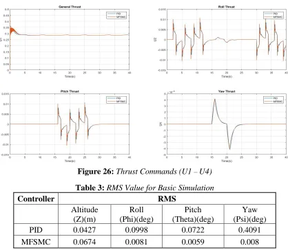
Figure 26: Thrust Commands (U1 – U4) ... 55

Figure 27: Simulink Diagram of the Sliding Mode Differentiator ... 58

Figure 28: Simulink Block for the Discrete Second-Order “Smoothing” Filter ... 58

Figure 29: Schematic of the Complimentary Filter Scheme [36] ... 60

Figure 30: Data Used for Noise Characteristic Estimation of Accelerometer and Gyroscope .... 61

Figure 31: Block Diagram for Coordinate Frame Conversion ... 65

Figure 32: Pitch Tracking and Tracking Error for the System Under PID and MFSMC ... 66

Figure 33: Roll Tracking and Tracking Error for the System Under PID and MFSMC ... 66

Figure 34: General Thrust (U1) for PID and MFSMC Controllers ... 67

Figure 35: Roll and Pitch Thrust (U2 – U3) for PID and MFSMC Controllers ... 67

Figure 36: Motor Commands (RPM) for PID and MFSMC Controllers ... 67

Figure 37: Switching Gains for the Roll and Pitch Tracking ... 68

Figure 38: Sliding Condition for the Roll and Pitch Tracking ... 68

Figure 39: Z (Altitude) Tracking and Tracking Error for PID and MFSMC ... 70

Figure 40: Roll Tracking and Tracking Error for PID and MFSMC ... 71

Figure 41: Pitch Tracking and Tracking Error for PID and MFSMC ... 71

Figure 42: Yaw Tracking for PID and MFSMC ... 72

Figure 43: Control Efforts (U1 – U4) for PID and MFSMC Controllers ... 72

Figure 44: Motor Commands (RPM) for PID and MFSMC Controllers ... 73

8

Figure 46: Sliding Condition for Altitude, Roll, Pitch and Yaw Tracking ... 74

Figure 47: Fusion 1 Quadcopter (from Craft Drones) ... 77

Figure 48: Spektrum Transmitter ... 77

Figure 49: Gimballed Fusion 1 Quadcopter ... 78

Figure 50: Quadcopter Experimental Roll Tracking and Tracking Error Responses ... 78

Figure 51: Quadcopter Experimental Pitch Tracking and Tracking Error Responses ... 79

Figure 52: Thrust Commands from Experimental Test ... 80

Figure 53: Motor Speeds from Experimental Test ... 81

Figure 54: Motor Speed Difference (mean subtracted) from Experimental Test ... 81

Figure 55: Sliding Condition for MFSMC from Experimental Test ... 82

Figure 56: MFSMC Switching Gains for the Experimental Test ... 82

Figure 57: Roll Tracking with Varying Lambda ... 83

Figure 58: Pitch Tracking for Varying Lambda ... 84

Figure 59: Sliding Condition for Roll and Pitch for Lambda = 1 (rad/sec) ... 85

Figure 60: Sliding Condition for Roll and Pitch for Lambda = 2 (rad/sec) ... 85

Figure 61: Sliding Condition for Roll and Pitch for Lambda = 3 (rad/sec) ... 86

9

LIST OF TABLES

Table 1: Controller Parameters for Second-Order Nonlinear MIMO System ... 35

Table 2: Quadcopter States [36]... 41

Table 3: RMS Value for Basic Simulation ... 55

Table 4: Power Consumption for Basic Simulation ... 56

Table 5: Accelerometer and Gyroscope Noise Estimation Characteristics ... 62

Table 6: RMS Value for Gimbal Simulation ... 69

Table 7: Power Consumption for Gimbal Simulation ... 69

Table 8: RMS Value for Full Model Simulation ... 74

Table 9: Power Consumption for Full Model Simulation ... 74

Table 10: RMS Value for Hardware Tracking Test ... 79

Table 11: Power Consumption for Hardware Tracking Test ... 79

10

NOMENCLATURE

UAS Unmanned Aerial System

UAV Unmanned Aerial Vehicle

SMC Sliding Mode Control

MFSMC Model Free Sliding Mode Control

IMU Inertial Measurement Unit

PID Proportional Integral Derivate

NED North-East-Down

B Control Input Gain

𝜆 Slope of the Sliding Surface

K Switching Gain

𝜑 Boundary Layer Thickness

Ф Roll Angle (°)

ϴ Pitch Angle (°)

Ψ Yaw Angle (°)

𝑢 Control Input

11

1.

INTRODUCTION

There has been a tremendous rise in the field of control systems used in system automation that is becoming more versatile for control highly complex systems. Control systems can be divided into linear and nonlinear control-type categories depending on the differential equations that govern the system behavior. Nonlinear systems are more complex and exhibit unpredictable behavior, requiring complex control algorithms [1]. A simple approach for nonlinear controls is to invert the nonlinear dynamics and replace it with the desired linear dynamics but requires the exact knowledge of the system model. If not known exactly, the inversion may lead to unstable residual dynamics [2]. In addition, effects of unmodeled dynamics (sensors and actuator dynamics) and external noise are also present and therefore, any nonlinear control schemes are required to be robust to such unknown perturbations.

Proportional-Integral Derivative (PID) control is the most popular theory used widely in industry applications. It is also used in complex systems like autonomous cars and Unmanned Aerial Vehicles (UAVs). The PID theory controls the systems states by compensating for the errors. But unfortunately, PID control strategies require definitive knowledge of the system model for proper tuning and are limited to linear and linearizable systems restricting its performance. Additionally, the PID controller needs to be properly tuned specific to each system that it is applied to resulting in a cumbersome and time consuming process.

12

The reaching phase drives the system towards a “sliding surface” and the sliding phase “slides” the states towards an equilibrium point. Lyapunov’s method is used to ensure asymptotic stability during the reaching phase. A discontinuous term is added to the control law to compensate for the system uncertainties and disturbances. However, the method requires knowledge of the mathematical model of the system and hence it is unique to each system which restricts its use. Therefore, there is a clear need to develop a Model-Free control algorithm based on the Sliding Mode Control (MFSMC) which derives the control law from previous control inputs, system measurements, control input gains and system’s order. An initial MFSMC control strategy was first proposed for Single-Input-Single-Output (SISO) systems [3] and then extended to Multi-Input-Multi-Output (MIMO) systems [4]. The goal of this research is to successfully integrate the proposed control algorithm on an Unmanned Aircraft System (UAS), e.g. quadrotor drone, for motion control and path tracking. In this work, a comparison in the performance of the proposed MFSMC algorithm to a traditional PID controller for tracking precision, power consumption and tuning time is presented.

13

2.

LITERATURE REVIEW

The literature review presents important conclusions of previous studies related to SMC, MFSMC and related control applications to UAS.

2.1

Generic SMC Schemes

Laghrouche et al. [5] introduced a higher-order sliding mode controller on optimal linear quadratic control applied to a minimum-phase nonlinear SISO systems. The problem was divided into three steps. First, a higher-order sliding mode problem was created to eliminate the chattering effect, followed by characterizing the nonlinear uncertainties as bounded non-structured parametric uncertainties considering the system as an uncertain linear system. Lastly, an optimal sliding mode controller was derived by minimizing a quadratic cost function over finite amount of time. The SMC was tested on a kinematic model of an automobile for steering controls from an initial position to a trajectory defined by the user. A sliding mode control of fourth-order was used with a time varying sliding surface. The system achieved perfect tracking with the error converging to zero with no chattering.

14

Runcharoon and Srichatrapimuk [7] presented an altitude control strategy for a quadrotor using a SMC system. The Euler angles was used to define the altitude (φ = roll, θ = pitch, ψ = yaw) and describe the orientation of the quadrotor. A PD controller was used to control the altitude (z) and the position (x and y) while the equations characterizing the positon and altitude were linearized to quantify the PD control gains. Euler angle assumptions φ ≈ ψ ≈ 0 on the x-axis, θ ≈ ψ ≈ 0 on the

y-axis and φ ≈ θ ≈ 0 were applied. A boundary layer was added to the dynamic equations to eliminate the control chattering about the sliding surface. The simulation was able to drive the quadrotor to the desired position and desired orientation and prove the stability of the system and the control inputs. The above authors [7] used a SMC and PD to achieve a stable closed-loop system. The strategy showed an improvement compared to a general PID control system, but it limited the full potential of a SMC which does not required linearization. The presence of under-actuated systems led to the use of two different control methods as it requires manipulation if used with the SMC process severely hindering the application of the proposed control scheme.

Sen et al. [8] introduced an adaptive method SMC for quadrotor helicopters. The work dealt with the estimation of the system uncertainties and perturbation bounds. As these bounds are unknown, they are overestimated thus leading to large gains and subsequently excessive control. The gain is directly proportional to the magnitude of chattering, and hence by estimating these bounds and updating the control law, the magnitude can be reduced. The method was implemented on a quadrotor helicopter. A stable closed-loop system with perfect position tracking with no chattering was achieved. The uncertainties bounds were unknown, which were later estimated.

15

Translational Oscillator with Rotational Actuator (TORA) and a quadrotor UAS. The quadrotor system was similar to the one used by Runcharoon and Srichatrapimuk [7] while the TORA was controlled using a rate bounded PID controller and a sliding mode controller [11]. A stable closed-loop convergence to the desired position was shown to be achieved.

Pai [12] demonstrated that the SMC showed robust tracking in discrete time systems by applying a discrete-time integral SMC on uncertain linear systems. An auxiliary control function was introduced to define the discrete-time sliding mode controller to stabilize the system. The switching surface was designed by extending the integral switching function from continuous to discrete time SMC ensuring quasi-sliding mode is reached [13, 14]. In practice, only the switching surface is approached by discrete-time SMC systems and hence quasi-sliding mode is assured. The method was applied to a discrete-time system and it showed excellent tracking performance with the presence of uncertainties along with stability of the closed-loop system. The integral switching surface in the design process eliminated the reaching phase and chattering was absent due to the absence of a switching gain.

16

Ferrara [16] presented the problem of applying SMC in systems with saturating actuators. A sub-optimal sliding mode controller with modifications was used to avoid control input saturation. The problem was the uncertainty in convergence of the sliding variable to zero in a finite amount of time when saturation occurs during reaching phase. The proposed modification decreases the control input magnitude once it reaches the saturation value (reaching phase). The control input magnitude increases again if the switching value was not reached implying the control input remains at the saturation value until a new switching value is reached. It is also proved that the system states converge to the origin in finite time and was reaffirmed with an example while avoiding the saturation limits.

2.2

Model–Free Sliding Mode Control Schemes

The limitation with strategies referenced previously is a system model is required for control development that is typically time consuming to design and also hinders performance in presence of model uncertainties. As dynamical systems become exceeding complex, a simplification is possible by developing a model-free control algorithm based on the sliding mode control.

Martinez-Guerra et al. [17] presented a Sliding Mode Observer (SMO) called master-slave synchronization to determine certain synchronization problem with chaotic behavior. The scheme required an accurate knowledge of the nonlinear system dynamics. Hence a model-free SMO with a promotional correction of the sign function of the synchronization error was introduced. The method was successful applied to the control of a Lorenz system (a nonlinear system exhibiting chaotic behavior when tuned to certain gains).

17

convergence of the desired trajectory, eliminating the need to know the system dynamics or parameters. Chattering was avoided to restrict damage to the actuators lifetime by using a higher-order SMC. However, the controller is integrated to a PD control whose desired gain values and performances requiring tuning. Two trajectories were tested: 1. sine wave; 2. triangular wave. A smooth response was achieved in both cases while the vehicle followed the desired path.

Raygosa-Barahona et al. [19] introduced a model-free back stepping technique with integral SMC to develop a model-free SMC system for under-actuated underwater Remotely Operated Vehicles (ROVs). A model-free controller was obtained by designing a regressor free second-order sliding mode controller as the auxiliary input control at each iteration. The sliding mode is integrated with a PID control and is applied to a ROV to track a helix trajectory. The vehicle states converged to the desired trajectory with no chattering. However, the PID controller requires tuning to achieve the desired performance.

18

Crassidis and Mizov [21, 22] presented a model-free control algorithm based on pure sliding mode control scheme to achieve perfect tracking for linear and nonlinear systems along with asymptotic tracking stability. The controller is designed based on previous control inputs, state measurements and the knowledge of the system order. A boundary layer was introduced into the control law to remove the excessive control chattering effect. The boundary layer reduced the tracking precision and gave a smooth control effort which is required. The method was tested on a first and second-order linear and nonlinear system. All the systems showed perfect tracking using identical controllers and outstanding asymptotic tracking stability was observed.

Crassidis and Reis [3] derived a similar model-free control algorithm based on SMC and extended the applications into SISO systems with non-unitary input gains. The effect of noise and system inaccuracies was also investigated. Firstly, a nonlinear mass-spring damper system with non-unitary control input gain without sensor noise was simulated followed by a state measurement noise using a Gaussian distribution of noise. The variance, mean and probability distribution was obtained from the sensor’s datasheet. Perfect tracking was obtained in both cases and chattering was eliminated by using a boundary layer.

19

quadrotor. The first system achieved perfect tracking on all states with the control effort maximized. But the latter observed perfect tracking on certain outputs while the control efforts and certain outputs displayed high frequency activity. This is due to the aggressiveness of the controller to track the required trajectory entirely. The presence of an actuator time delay had an adverse effect when it exceeded 0.1 seconds. Hence the control law needs to be modified to account for the presence of this time delay. The modified control law handled the time delay inaccuracies but was inconsistent at 0.1 seconds of time delay in some cases.

Levant [23] also presented a unique method of model-free sliding mode control based on Higher Order Slide Mode [HOSM] theory. The controller form is based usually on an insignificant relay controller 𝑢 = −𝐾𝑠𝑔𝑛(𝑆) where 𝑆 = 𝑥 − 𝑥𝑑 satisfies the higher-order sliding modes. No

information about the plant and only the relative order (r) is required for the controller since S and its derivatives are based only on the states. The control effort is calculated by integration eliminating the chattering effect without the need for a smoothing step. The method eliminates chattering in the ideal scenario, but chattering may still be present due to the excitation of parasitic dynamics [24]. The parasitic dynamics are unmodeled dynamics such as actuator or sensor delays. The control law was successfully used to steer a four-wheeled vehicle onto a desired trajectory.

Precup [25] developed two distinct methods of model-free sliding mode control based on dynamic data-driven linear estimation of the system model. For a first-order system, the sliding surface is defined as:

𝑆 = 𝑥̃(𝑡) + ∫ 𝑥̃(𝜏)𝑑𝜏

𝑡

0

20

𝑦̇(𝑡) = 𝐹(𝑡) + 𝛼𝑢(𝑡)

where α is a tunable parameter. It is selected to keep the magnitude of 𝑦̇ and 𝑢 same. F(t) is approximated to:

𝐹̂(𝑡) = 𝑦̂(𝑡) − 𝑢(𝑡)

where 𝑦̂(𝑡) is determined from y by a first-order derivative and a low-pass filter. Replacing the discontinuous sign function and adding a thickness boundary layer and a saturation function, the SMC control law was derived as:

𝑢 = 𝛼−1(−𝐹̂(𝑡) + 𝑥̇𝑑(𝑡) − 𝜆−1𝑥̃(𝑡) − 𝑒𝑒𝑠𝑡 𝑚𝑎𝑥− 𝜆−1𝑠𝑎𝑡(𝑆 𝜑⁄ ))

where eest max satisfies the following inequality:

𝜑−1_{|𝑆(𝑡)|𝜂 > 2𝜆𝑒} 𝑒𝑠𝑡 𝑚𝑎𝑥

The method is similar to those used in [3, 4, and 21] as it is the adaption of conventional SMC with the system model estimated from only the states and inputs. However, in this method the algebraic loops are avoided using a differentiator rather than a direct state measurement.

2.3

Sliding Mode Control for Under-actuated System

21

Qian, Yi and Zhao [27] developed a multi-surface SMC for a single-input multi-output under-actuated system. The proposed method was based on nested sliding variables including all system states. The number of sliding surfaces depends on the number of states. It allows tracking of multiple outputs with a single input. Tunable coefficients were weighted to the outputs to lower leveled sliding surfaces when constructing higher leveled sliding surfaces. The method was validated through a simulation effort on a single and double inverted pendulum for stabilization. The effect for chattering was not mentioned nor handled.

Schkoda [28] developed a squaring transformation diffeomorphism using optimal control theory to decide the weighting of different outputs in the transformation. The method is similar to the approach developed by Raygosa [19]. Virtual control inputs were mapped to the actual control inputs through a transformation diffeomorphism. The transformation matrix in [28] led to a square input matrix which is inverted to derive the SMC control law for MIMO systems.

One major area of application of under-actuated systems is in Unmanned Aircraft Systems (UASs). There are two main configurations of UASs, fixed-wing and quadrotor. Fixed-wing UASs are similar in nature to conventional aircraft. The four traditional control inputs are the rudder, elevator, ailerons, and forward thrust (engine). A quadrotor is a type of helicopter with four equal-sized rotors distributed equally in horizontal plane around the center-of-mass. Typical the rotors employ a fixed blade pitch and implies that torque is the only input. The next section reviews some methods used to develop SMC for UAS addressing the issue of under-actuation.

2.4

Sliding Mode Control for Unmanned Aircraft Systems

22

diffeomorphism to the differential equations of the systems. After coordinate transformations, the differential equations are given as four three dimensional equations zi, with four sliding variables

Si defined as:

𝑆_𝑖 = 𝑧_𝑖 − 𝑧_𝑖𝑑, i =1, 2, 3, 4

In the approach, 𝑧_𝑖𝑑is the desired trajectory to be tracked in the transformed coordinate system. Similar to classic SMC, the sliding variables are differentiated and substituted in the system model. The control laws are developed for thrust and surface deflections along with three virtual controllers to compensate modal uncertainties.

Abdulhamitbilal [30] also developed 6 DOF state-space model for a fixed-wing UAS with 12 states. Unlike assigning a sliding surface to each state as proposed in [14], only four sliding surfaces were developed, one for each input (rudder, elevator, aileron deflections and thrust). The two 6-dimensional state variables (position and velocity) are transformed into a 4-dimensional space with the sliding surface. Transformation matrix using weights for individual states like the one used in [28] is used.

Duan, Mora-Camino and Miquel [2] compared the performance of a decoupled longitudinal fixed-wing UAS model using dynamic inversion and backstepping methods. A full 6 DOF aircraft model with actuator dynamics was simulated but only the longitudinal results were examined. The backstepping method gave smoother responses but the control law was extremely complex and cumbersome to implement.

23

yaw (heading) angle and orthogonal distance from the required path. Even though the system was under-actuated, the proposed control law was able to regulate both outputs effectively.

Villanueva et al. [32] developed a 6 DOF state-space model for a quadrotor with 12 states. Four different control modes (manual, altitude hold, position hold, and waypoint following) was derived using the super-twisting method of SMC. The under-actuation of the quadrotor was resolved by the addition of pseudo-control inputs to roll and pitch that are dependent on positions in the horizontal plane. The approach was the same method used by Munoz-Vazquez et al. [20] where pitch and roll were removed as the explicit outputs of the system and the remaining 4 states and 4 inputs transform the problem to a fully actuated system. The proposed method is different to the method followed in [4] where all 6 DOF were retained and a transformation matrix was used for the under-actuated system using tracking weights.

Derafa, Benallegue, and Fridman [33] also applied super-twisting on a quadrotor and tested the system in a real-world application. The controller was developed for attitude tracking and stabilization. The desired values are given as functions of desired positions. The system modelled in this method becomes a fully actuated system.

24

observed for both the PID and MFSMC controller. Improved state estimation and system characterization was suggested to improve the tracking performance and reduce tracking error.

25

3.

MODEL FREE SMC ALGORITHM

In this chapter, the derivation for the MFSMC algorithm as proposed in [3, 4] and its application on a second-order nonlinear system is presented. The first section describes the stability of nonlinear systems, autonomous and non-autonomous systems, and square and non-square systems. In the next section, the model-free control algorithm for squared second-order systems followed by the application of the control algorithm on nonlinear systems is developed.

3.1 Lyapunov Stability Theory

Russian mathematician Alexandr Lyapunov introduced the Lyapunov theory to analyze system stability for linear and nonlinear systems [35]. The theory introduces two methods: 1. the Linearization Method and; 2. the Direct Method. The first method linearizes a nonlinear system around an operating point condition and analyzes the stability of the system at that point. The Direct Method uses the concept of energy to quantify stability. The sliding mode control utilizes the Direct Method ensure tracking stability the derived closed-loop control system.

3.1.1 Autonomous and Non-Autonomous Systems

A nonlinear system is said to be autonomous if the system parameters do not depend explicitly on time (Slotine [1]), and is defined as:

𝑥_𝑝𝑛 _{= 𝑓}

𝑝(𝑥; 𝑢𝑚) (1)

26

3.1.2 Equilibrium Points

An equilibrium point is defined as the point where the system’s state trajectories converge to a steady-state condition. Linear systems have one equilibrium point at the origin while nonlinear systems can have several or infinite equilibrium points. The equilibrium point is defined as:

𝑓_𝑝(𝑥_𝑝𝑒) = 0 (2)

Consider the nonlinear equation of motion of a pendulum:

𝑀𝑅2_{𝛳̈ + 𝑏𝛳̇ + 𝑀𝑔𝑅 𝑠𝑖𝑛 𝛳 = 0 (3)}

where, M is mass of the pendulum, R is the length of the pendulum, ϴ is the angle between the pendulum and the vertical, b is coefficient of friction, and g is the acceleration due to gravity.

The state-space equation for the system is:

𝑥̇1 = 𝑥2 (4)

𝑥̇₂ = − 𝑏

𝑀𝑅2𝑥2−

𝑔

𝑅𝑠𝑖𝑛 𝑥1 (5)

where, 𝑥₁ = 𝑛𝜋 are the infinite number of equilibrium points for the pendulum.

3.1.3 Concepts of Stability

An equilibrium point is stable if given a spherical region with radius R > 0, there exists 𝑟 > 0, such that if ‖𝑥(0)‖ < 𝑟, then ‖𝑥(𝑡)‖ < 𝑅 for all 𝑡 ≥ 0. Otherwise, the equilibrium point is unstable. The is referred to as Lyapunov stability and outlined in Slotine [1].

An equilibrium point (𝑥𝑒) is said to be asymptotically stable if it is stable as defined above and

there exists some 𝑟 > 0 such that ‖𝑥(0)‖ < 𝑟 and 𝑥(𝑡) → 𝑥_𝑒 as 𝑡 → ∞. If there exist a point ‖𝑥2‖ < 𝑅 and 𝑥(𝑡) → 𝑥2 as 𝑡 → ∞, then the point is marginally stable. If doesn’t meet either of

27

Figure 1: Concepts of Stability [1]

Apart from convergence to the equilibrium point, estimates of how fast the trajectories converge to the equilibrium point are also important. An equilibrium point is said to be exponentially stable if there exist two positive numbers α and δ such that for 𝑡 > 0, ‖𝑥(𝑡)‖ ≤ 𝛼‖𝑥(0)‖𝑒−𝛿𝑡, inside of

SR. The concept proves that the state vector is converging faster than the exponential function to the equilibrium point.

The equilibrium point is said to be globally asymptotically or exponentially stable if asymptotic or exponential stability hold for any and all initial states in the large.

3.1.4 Lyapunov’s Direct Method

28

The energy function has certain rules to be considered. The function 𝑉(𝑥) must be strictly positive for all 𝑥 and 𝑥̇ excluding the origin. The function 𝑉(𝑥) is said to be positive definite if 𝑉(𝑥) > 0 for any 𝑥 ≠ 0.𝑉̇(𝑥) is said to be negative semi-definite if 𝑉̇(𝑥) ≤ 0. If these conditions are met then the equilibrium point is said to be stable.

The equilibrium point is said to be asymptotically stable if 𝑉(𝑥) is strictly positive definite and 𝑉̇(𝑥) is strictly negative definite. The equilibrium point is globally asymptotically stable, if 𝑉(0) = 0, 𝑉(𝑥) > 0 for any 𝑥, 𝑉̇(𝑥) < 0 for any 𝑥, and 𝑉(𝑥) is radially unbounded.

3.2 Model Free Sliding Mode Control Scheme

Reis and Crassidis [3] derived a model-free SMC law for SISO linear and nonlinear first and second-order systems with unitary and non-unitary gains. The developed control law testing using simulations for various systems and perfect state tracking was shown to be achieved. El Tin and Crassidis [4] extended the previous work to MIMO linear and nonlinear first and second-order squared and non-squared systems with non-unitary gains. Perfect state tracking and asymptotic tracking stability was achieved in the simulations. In this section, the definitions of squared and non-squared MIMO systems are defined and the MFSMC algorithm for second-order squared MIMO system is derived.

3.2.1 Square and Non-square MIMO Systems

To derive the control law for MIMO systems, the various types of MIMO systems should be considered. Also, the control input gain matrix [B] needs to be invertible for the control law to be derived.

29

𝑥_𝑝𝑛 = 𝑓_𝑝(𝑥) + [𝐵]_𝑝×𝑚𝑢_𝑚 (6) where p and m are the number of outputs and inputs respectively, 𝑥 is the system states and output,

fp(x) is the autonomous nonlinear character in 𝑥, B is the p x m control input matrix gains, and u is the control input.

A system whose number of inputs is equal to the number of outputs (i.e., m = p) is called a square or fully actuated system. Each output system has its own controller and perfect control can be achieved assuming the system is controllable.

When the number of inputs is greater than output (m > p) the system is referred to as a non-square system, and is considered over-actuated. In this case, we have an abundance of control inputs and one controller can be replaced by another one.

The non-square system where the number of inputs is less than outputs (m < p) is referred to as an under-actuated system. In the non-square systems, the control input matrix [B] is not invertible hence further manipulation is required to derive the model-free control algorithm based on the SMC.

3.2.2 System Description for Squared MIMO Systems

Consider the nth order autonomous system:

𝑥_𝑝𝑛 = 𝑓_𝑝(𝑥) + [𝐵]_𝑝×𝑚𝑢_𝑚 (7) The system description can be rewritten as:

𝑥𝑝𝑛 = 𝑥𝑝𝑛 + [𝐵]𝑢𝑚− [𝐵]𝑢𝑚𝑘−1− [𝐵]𝑢𝑚+ [𝐵]𝑢𝑚𝑘−1 (8)

30

input. The error between the control input and the previous control input is defined as:

𝜀_𝑚 = 𝑢_𝑚𝑘−1 − 𝑢_𝑚 (9) To avoid an algebraic loop within the controller algorithm and to compute the control law, a control input error estimation function is required and is defined as

𝜀 _𝑚 = 𝑢_𝑚𝑘−1− 𝑢_𝑚𝑘−2 (10) where, 𝑢_𝑚𝑘−2 is the previous control input of the previous control input. The control input error is not exactly known but it is assumed to be within the following bounds:

(1 − 𝜎𝑙)𝜀 𝑚 ≤ 𝜀 𝑚≤ (1 + 𝜎𝑙)𝜀 𝑚 (11)

where 𝜎𝑢 is the upper bound and 𝜎𝑙 is the lower bound of the control input estimation error.

The control input gain [B] is unknown but is assumed to be bounded, i.e.,:

𝑏_{𝑙𝑜𝑤𝑒𝑟} ≤ 𝑏_𝑚𝑚≤ 𝑏_{𝑢𝑝𝑝𝑒𝑟} (12)

where blower is the lower most bound, bupper is the upper bound and bmm is an element of the control input gain matrix [B].

3.2.3 Second Order MIMO System Control Law

A possible time varying sliding surface can be defined as [1]:

𝑠𝑚= ( 𝑑

𝑑𝑡+ 𝜆𝑚) 𝑛−1_𝑥̃

𝑝 (13)

where λm is a positive constants, n is the order of the system, and 𝑥̃𝑝 = 𝑥𝑝− 𝑥𝑑𝑝 defines the

tracking error.

The sliding surface for a second-order MIMO system is then defined as:

31

By setting the derivative of the sliding surface is to zero ensures the state trajectories remain on the sliding surface on the trajectories have reached the surface, i.e.,:

𝑠⃗̇ = 𝑥⃗̃̈ + 𝜆𝑥⃗̃̇ = 0⃗⃗ (15) Substituting Eq. (8) into Eq. (13) results in:

𝑠⃗̇ = 𝑥⃗̈ + [𝐵]𝑢⃗⃗ − [𝐵]𝑢⃗⃗_𝑘−1+ [𝐵]𝜀⃗ − 𝑥⃗̈_𝑑+ 𝜆𝑥⃗̃̇ = 0⃗⃗ (16) Rearranging the equation for the control input and adding the discontinuous term to eliminate the system uncertainties results in:

𝑢⃗⃗ = −[𝐵]−1[𝑥⃗̈ − 𝑥⃗̈𝑑+ 𝜆𝑥⃗̃̇ + 𝜂𝑠𝑔𝑛(𝑠⃗)] + 𝑢⃗⃗𝑘−1− 𝜀⃗ (17)

where 𝜂 is assumed to be a small positive constant.

3.2.4 Asymptotic Stability of the Control Law

Lyapunov’s Direct Method is used to achieve asymptotic stability of the control law during the reaching phase. A candidate Lyapunov function that is strictly positive definite (satisfying one of the Direct Method stability criterion) can be defined as:

𝑉⃗⃗(𝑥⃗) = 1

2𝑠⃗

2 ₍₁₈₎

Differentiating Eq. (16) results in:

𝑉⃗⃗̇(𝑥⃗) = 𝑠⃗̇𝑠⃗ (19) Substituting Eq. (14) into Eq. (1) and setting Eq. (17) to be strictly negative to ensure global asymptotic stability results in:

32

𝑉⃗⃗̇(𝑥⃗) = 𝑠⃗ (𝑥⃗̈ + [𝐵] (−[𝐵]−1[𝑥⃗̈ − 𝑥⃗̈_𝑑+ 𝜆𝑥⃗̃̇ + 𝜂𝑠𝑔𝑛(𝑠⃗)] + 𝑢⃗⃗_𝑘−1− 𝜀⃗) − [𝐵]𝑢⃗⃗_𝑘−1+

[𝐵]𝜀⃗ − 𝑥⃗̈𝑑 + 𝜆𝑥⃗̃̇ ) ≤ 0 (21)

Simplifying Eq. (19) results in:

𝑉⃗⃗̇(𝑥⃗) = 𝑠⃗(−𝜂𝑠𝑔𝑛(𝑠⃗)) ≤ 0 (22) The signum function gives negative unity when the sliding surface is negative and positive unity when the sliding surface is positive. The term “ 𝑠⃗(𝑠𝑔𝑛(𝑠⃗))” can be replaced with “|𝑠⃗|” yielding:

𝑉⃗⃗̇(𝑥⃗) = −𝜂|𝑠⃗| ≤ 0 (23) which is always satisfied as η is strictly positive. This ensures the derivative of the Lyapunov function as negative definite and therefore the asymptotic stability of the system is achieved.

3.2.5 The Switching Gain

The control law Eq. (15) is formally now updated with the switching gain, i.e.,:

𝑢⃗⃗ = −[𝐵̂]−1_{[𝑥⃗̈ − 𝑥⃗̈}

𝑑+ 𝜆𝑥⃗̃̇ + 𝐾⃗⃗⃗𝑠𝑔𝑛(𝑠⃗)] + 𝑢⃗⃗𝑘−1− 𝜀⃗ (24)

where the switching gain 𝐾⃗⃗⃗ ensures that the state trajectories are asymptotically stable during the reaching phase and [𝐵̂] is the estimate of the control input gain matrix.

Using the sliding condition defined in Eq. (21), the asymptotic stability of the closed-loop system is ensured so that:

𝑠⃗̇𝑠⃗ ≤ −𝜂|𝑠⃗| (25)

33

𝐾⃗⃗⃗ = |𝑥⃗̈ − 𝑥⃗̈_𝑑||[𝛽] − 1| + 𝜆|𝑥⃗̃|̇|[𝛽] − 1| + |[𝐵̂]𝜎_𝑢(𝑢⃗⃗_𝑘−2− 𝑢⃗⃗_𝑘−1)| + [𝛽]𝜂 (26)

The control law in Eq. (22) is updated as:

𝑢⃗⃗ = −[𝐵̂]−1[𝑥⃗̈ − 𝑥⃗̈_𝑑+ 𝜆𝑥⃗̃̇ + 𝐾⃗⃗⃗𝑠𝑔𝑛(𝑠⃗)] + 2𝑢⃗⃗_𝑘−1− 𝑢⃗⃗_𝑘−2 (27) The estimated control input gain is given by the geometric mean of the upper and lower bounds:

[𝐵⃗⃗̂] = √𝑏𝑢𝑝𝑝𝑒𝑟𝑏𝑙𝑜𝑤𝑒𝑟 (28)

The auxiliary variable β is defined as:

𝛽 = 𝑏̂𝑏̂−1= √𝑏𝑢𝑝𝑝𝑒𝑟

𝑏𝑙𝑜𝑤𝑒𝑟 (29)

3.2.6 The Boundary Layer

The discontinuous term in the control law shown in Eq. (25) causes high frequency chattering of the control effort [3, 4] causing damage to the actuators and motors in the real-world. Hence, a smoothing boundary layer is added into to the control law and the algorithm is formulated as:

𝑢⃗⃗ = [𝐵]−1_{[−𝑥⃗̈ + 𝑥⃗̈}

𝑑− 𝜆𝑥⃗̃̇ − (𝐾⃗⃗⃗ − 𝛷⃗⃗⃗̇)𝑠𝑎𝑡 ( 𝑠⃗ 𝛷

⃗⃗⃗⃗)] + 2𝑢⃗⃗𝑘−1− 𝑢⃗⃗𝑘−2 (30)

where the boundary layer dynamics are defined as follows (Slotine [1]):

𝛷⃗⃗⃗̇ + 𝜆𝛷⃗⃗⃗ = 𝐾⃗⃗⃗(𝑥⃗_𝑑) (31) with 𝛷⃗⃗⃗(0) = η/λ. The control effort smoothing approach is similar to applying a “perfect” first-order filter with zero phase loss to the control effort.

3.3 Second Order System Illustration

34 The equation of motion of system was defined by:

𝑚₁𝑥̈₁ = 𝑢₁+ 𝑐₂(𝑥̇₂− 𝑥̇₁)|𝑥̇₂− 𝑥̇₁| + 𝑘₂(𝑥₂− 𝑥₁) − 𝛽₂(𝑥₂− 𝑥₁)3_{− 𝑐}

1𝑥̇1|𝑥̇1| − 𝑘1𝑥1

+ 𝛽₁𝑥₁3

𝑚2𝑥̈2 = 𝑢2− 𝑐2(𝑥̇2− 𝑥̇1)|𝑥̇2− 𝑥̇1| − 𝑘2(𝑥2− 𝑥1) − 𝛽2(𝑥2− 𝑥1)3

where mi is the mass, 𝑥_𝑖 is the state output, ui is the input, ci (𝑐⃗ = [5,8]´) is the damping coefficient,

ki (𝑘⃗⃗ = [3,7]´) is the spring constant, βi (𝛽⃗ = [−1.5, −3]´) is the spring stiffening coefficient and

i is the number of masses, springs and dampers.

The control input gain is [B] = [1/m1, 1/m2] ´ with known bounds:

5 ≤ 𝑚1 ≤ 15

15 ≤ 𝑚₂ ≤ 25

The signals to be tracked are:

𝑥_1𝑑(𝑡) = sin (𝜋

35 𝑥2𝑑(𝑡) = sin (

𝜋 2𝑡)

The same controller parameters used in [4] was used and are given below:

Table 1: Controller Parameters for Second-Order Nonlinear MIMO System

Parameter Value 𝜎𝑢 0.5

𝜆 20

𝜂 0.1

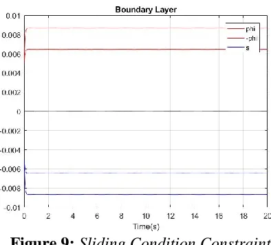
The closed-loop simulation results with the derived control law are given below:

36

Figure 3: Position Tracking Error of (1) X1, (b) X2

Figure 4: Velocity Tracking of (a) X1, (b) X2

37

Figure 6: Acceleration Tracking of (a) X1, (b) X2

38

Figure 8: Controller Effort (a) U1, (b) U2

Figure 9: Sliding Condition Constraint

39

4.

METHODOLOGY

The objective of this work is to implement the exclusive and unique model-free control algorithm on real-world hardware and to compare the performance to a traditional PID controller with respect to tracking precision and power consumption. The Root-Mean-Square (RMS) of the tracking error (desired trajectory – actual trajectory) is used to compare the tracking performance. As shown in Section 2, to date there has been no work that has used the MFSMC on a real hardware successfully. Schulken [34] implemented the developed MFSMC on an actual hardware but the performance was unacceptable. A quadcopter was selected for hardware implementation in this study. More details about the hardware are mentioned later in Chapter 6.

In Chapter 5, the simulation study of the quadcopter with both PID and MFSMC law is presented. Simulations are used to study system behavior and performance prior to implementing the newly developed control strategy on actual hardware. This identifies critical system (model errors, actuator dynamics, Inertial Measurement Unit (IMU) errors and sensor noise) behavior that could cause damage or lead to hardware damage during flight testing and saves valuable time and effort during hardware development. The simulation study was conducted on a basic quadcopter dynamic model followed with including hardware components such as actuator dynamics, sensor delays, state estimation, IMU sensor noise and controller sampling frequency.

40

5.

SIMULATION STUDY

This chapter describes the simulation studies conducted on the dynamic model of a quadcopter with the proposed MFSMC algorithm and the PID controller. The chapter is divided into six sections. The first section describes the dynamic model of the quadcopter and delves into the plant model states, the reference frames, the various quadcopter orientation configurations, the plant model equations, the thrust equations, and the motor dynamics of a basic quadcopter. The second section characterizes the actuator dynamics required in the proposed MFSMC algorithm followed by the basic simulation testing (shown in the third section) of the MFSMC algorithm and the predesigned PID controller on the quadcopter model developed in first section of the chapter. The design of the control law in the MFSMC algorithm to actuator efforts is important as mentioned by El Tin [4]. The fourth section describes state estimation that is required for hardware implementation followed by state conversion into body-reference frame components outlined in the fifth section of this chapter. Noise characterization of signals sensed by the IMU is illustrated in final section with MFSMC algorithm parameter selection as mentioned by Reis [3]. Finally, a simulation study of real-world hardware is carried out under the MFSMC law and the performance is compared to a traditional PID controller for a quadcopter.

5.1 Quadcopter Plant Model

5.1.1 Plant Model States

The quadcopter is a 6 DOF system that travels in the X, Y and Z directions and rotates about the X

41

Figure 10: Quadcopter State Coordinate Visualization [36]

Quadcopters have various sensors that measure the different states of the quadcopter. The sensors include accelerometers, gyroscopes, vision, GPS etc. A state that can be directly measured using a sensor is referred to as a fully observable state. The quadcopter used in this study uses an IMU which comprises of a full 3-axis accelerometer and gyroscope. The states of the quadcopter are described in Table 2.

Table 2: Quadcopter States [36]

Symbol Description Unit Observability

𝜃 Pitch Euler Angle 𝑟𝑎𝑑 Stereo Vision

𝜃̇ Pitch Euler Angular Velocity 𝑟𝑎𝑑/𝑠 Gyroscope 𝜃̈ Pitch Euler Angular

Acceleration

𝑟𝑎𝑑 /𝑠2 _-

𝜙 Roll Euler Angle 𝑟𝑎𝑑 Stereo Vision

𝜙̇ Roll Euler Angular Velocity 𝑟𝑎𝑑/𝑠 Gyroscope 𝜙̈ Roll Euler Angular Acceleration 𝑟𝑎𝑑 /𝑠2 _-

𝜓 Yaw Euler Angle 𝑟𝑎𝑑 Stereo Vision

𝜓̇ Yaw Euler Angular Velocity 𝑟𝑎𝑑/𝑠 Gyroscope 𝜓̈ Yaw Euler Angular

Acceleration

𝑟𝑎𝑑 /𝑠2 _-

42

𝑋̇ Velocity along X 𝑚/𝑠 -

𝑋̈ Acceleration along X 𝑚 /𝑠2 _{Accelerometer}

𝑌 Position along Y 𝑚 Stereo Vision

𝑌̇ Velocity along Y 𝑚/𝑠 -

𝑌̈ Acceleration along Y 𝑚 /𝑠2 _{Accelerometer}

𝑍 Position along Z 𝑚 Stereo Vision

𝑍̇ Velocity along Z 𝑚/𝑠 -

𝑍̈ Acceleration along Z 𝑚 /𝑠2 _{Accelerometer}

Ω1 Motor 1 Angular Velocity 𝑟𝑎𝑑/𝑠 Voltage/Current/Optical Ω2 Motor 2 Angular Velocity 𝑟𝑎𝑑/𝑠 Voltage/Current/Optical Ω3 Motor 3 Angular Velocity 𝑟𝑎𝑑/𝑠 Voltage/Current/Optical Ω4 Motor 4 Angular Velocity 𝑟𝑎𝑑/𝑠 Voltage/Current/Optical

5.1.2 Reference Frames and Orientations

The two reference frames are assumed to be: 1. local NED (North – East – Down) reference frame and; 2. body-reference frame. The NED reference is an inertial frame while the body-reference frame is a non-inertial frame and is assumed fixed on the UAS and moves along with the UAS as the UAS maneuvers in a 3D space.

43

Figure 11:Local NED Right Handed Frame [36]

The body-reference frame is dependent on the orientation of the quadcopter. Generally the quadcopter has two orientations: 1. ‘+’ orientation and; 2. ‘X’ Orientation. The direction of positive Z is common in both orientations and acts downwards. The difference in the orientations depends on the direction of the X and Y axes and the motors used to change direction. In this study, the ‘X’

orientation is used. The body-reference frame for both orientations are:

44

5.1.3 Plant Model Equations

In this section, a mathematical model of the 6 DOF quadcopter is presented as shown in [4, 9, 34, and 36] to develop a full quadcopter system model. The assumptions for the model are [36]:

• The quadcopter is a rigid structure;

• The air frame and components are symmetric;

• The center-of-gravity and air frame origin coincide;

• Thrust and drag are proportional to the square of propeller speed;

• There are no external disturbances, i.e., wind, temperature etc. acting on the quadcopter.

First, the angular accelerations of the quadcopter are modeled. These include all the moments acting on the quadcopter, i.e., the rolling moments, pitching moments and yawing moments. Each of the moments consists of the following effects:

• Body gyroscopic effects – changes in quadcopter orientation;

• Propeller gyroscopic effects – propeller rotation with quadcopter frame orientation;

• Actuation effects – forces produced by rotor.

The sum of these effects in the respective axes output the angular accelerations for roll (Ф), pitch (ϴ) and yaw (ψ). Figure 14 illustrates the effects in the acceleration equations.

45

Similarly, the pitch and yaw angular accelerations can be generated. The three angular accelerations used for in the quadcopter model are given below:

Ф̈ = 𝛳̇𝜓(𝐼𝑦𝑦−𝐼𝑧𝑧)+ 𝐽𝑟𝛳̇𝛺𝑟+𝑙𝑈2

𝐼𝑥𝑥 (32)

𝛳̈ = Ф̇𝜓̇(𝐼𝑧𝑧−𝐼𝑥𝑥)+ 𝐽𝑟Ф̇𝛺𝑟+𝑙𝑈3

𝐼𝑦𝑦 (33)

𝜓̈ = 𝛳̇Ф̇(𝐼𝑥𝑥−𝐼𝑦𝑦)+𝑈4

𝐼𝑧𝑧 (34)

where U2, U3 and U4 are roll, thrust and yaw thrust respectively. Ωr is total velocity of all the propellers and will be discussed further in the next section. 𝐼_𝑥𝑥, 𝐼_𝑦𝑦 and 𝐼_𝑧𝑧 are the moment-of-inertias (Kg-m2) terms, Jr is the rotor inertia of the motors (Kg-m2) and, l is the distance between the rotor axis and quadcopter center-of-mass.

Similarly, the accelerations along the translational axes can be defined. Figure 15 depicts the different aspects of the acceleration equations.

Figure 15: Acceleration Equation along the “X” Direction [36]

By following a similar approach the accelerations in Y and Z can be defined. The three translational accelerations are given as:

𝑋̈ =(𝑠𝑖𝑛 𝜓 𝑠𝑖𝑛 Ф− 𝑐𝑜𝑠 𝜓 𝑠𝑖𝑛 𝛳 𝑐𝑜𝑠 Ф)𝑈1−𝐴𝑥𝑋̇

46

𝑌̈ =(𝑐𝑜𝑠 𝜓 𝑠𝑖𝑛 Ф− 𝑠𝑖𝑛 𝜓 𝑠𝑖𝑛 𝛳 𝑐𝑜𝑠 Ф)𝑈1−𝐴𝑦𝑌̇

𝑚 (36)

𝑍̈ =𝑚𝑔−(𝑐𝑜𝑠 𝛳 𝑐𝑜𝑠 Ф)𝑈1−𝐴𝑧𝑍̇

𝑚 (37)

where Ax, Ay, and Az are the air resistances in the respective axes (kg/s), U1 is the general thrust and m is the mass of the quadcopter (kg). Eqs. (30 – 35) finalize the mathematical model of the 6 DOF quadcopter model. The system equations are referenced to the local NED reference frame and are used for simulation study to evaluate the MFSMC performance.

5.1.4 Thrust Equations

There are four main thrust equations that should be considered for inclusion in the model. The thrust variables were included in the plant model equations in the previous section. The four thrust parameters are the general thrust (U1), roll thrust (U2), pitch thrust (U3), and yaw thrust (U4). The thrust equations are required to model the individual rotor characteristics that drive and control the quadcopter and are orientation dependent. The thrust equations with respect to the ‘X’ orientation

are given as follows:

𝑈1 = 𝑏(𝛺₁2+ 𝛺₂2 + 𝛺₃2+ 𝛺₄2) (38)

𝑈2 = 𝑏 𝑠𝑖𝑛(𝜋

4) (𝛺1

2 _{− 𝛺}

22− 𝛺32+ 𝛺42) (39)

𝑈3 = 𝑏 𝑠𝑖𝑛(𝜋

4) (𝛺1 2

+ 𝛺22− 𝛺32− 𝛺42) (40)

𝑈4 = 𝑑(𝛺12− 𝛺22+ 𝛺32− 𝛺42) (41)

47

Figure 16: Thrust Equations in Along the 'X' Orientation [36]

For example, as shown in Figure 16, U1 applies a general thrust which is uniform and equal to each of the motors that drive the individual rotors. U2 changes the thrust between the motors to roll the quadcopter while U3 changes the thrust between motors to pitch the quadcopter. Similarly,

U4 is used to yaw the quadcopter.

The overall angular velocity of the quadcopter is given as:

48

5.1.5 Motor Dynamics

Motor dynamics play an important role in the system dynamics as they cause actuator delays in the closed-loop system. To understand the motor behavior and characteristics, the dynamics must be modeled into the quadcopter model. A brushless DC motor with a controller is modeled to ensure the motor is operating at the proper desired angular velocity. The inputs to the motor are voltage and desired angular velocity (calculated in the previous section). The motor states are current and angular acceleration and the output of the motor is angular velocity. The motor modeling equations are given as:

𝐿𝑑𝑖

𝑑𝑡= 𝑉 − 𝑅𝐼 − 𝐾𝑒𝑚𝑓𝛺 (43)

𝐽𝑑𝜔

𝑑𝑡 = 𝐾𝑡𝐼 − 𝑏𝜔 (44)

where L in the electrical inductance (H), I is the current (ohm), V is the voltage (V), R is the electrical resistance (ohm), Kemf is the back electromotive force coefficient (V-s/rad), J is the rotor moment-of-inertia (kg-m2), Kt is the torque coefficient (Nm/A), and b is the damping coefficient (N-m-s). The Simulink block model of the motor is shown in Figure 17.The saturation blocks limits the voltage and current as supplied by the battery.

49

5.2 Control Approach for Quadcopter

Depending on the number of degree-of-freedoms to be controlled, the control system can be treated as either a fully actuated or under-actuated system. Xu [9], El Tin [4] and Schulken [34] controlled

X, Y, Z and ψ (yaw) in their simulation studies and considered the under-actuated system approach. Xu and El Tin used U1 to control the altitude Z and U4 to control yaw angle (ψ). U2 and U3 were used to control X and Y, respectively. El Tin used a transformation diffeomorphism approach to convert the under-actuated system into a fully actuated system [4].

Schulken [34] used the super-twisting approach to control X and Y while the altitude and yaw were directly controlled by the control inputs and was the same approach used in [32 and 33]. In this work, the pseudo-control Ux and Uy signals are generated from the desired X and Y commands. The pseudo-inputs can be considered as the portion of U1 on the horizontal and vertical direction. The pseudo-inputs are defined by the following:

𝑈_𝑥 = 𝑠𝑖𝑛 Ф 𝑠𝑖𝑛 𝜓 + 𝑐𝑜𝑠 Ф 𝑠𝑖𝑛 𝛳 𝑐𝑜𝑠 𝜓 (45)

𝑈_𝑦 = − 𝑠𝑖𝑛 Ф 𝑠𝑖𝑛 𝜓 + 𝑐𝑜𝑠 Ф 𝑠𝑖𝑛 𝛳 𝑐𝑜𝑠 𝜓 (46) These inputs are used to define the required roll and pitch angles using the following:

Ф𝑑 = 𝑠𝑖𝑛−1(𝑈𝑥𝑠𝑖𝑛(𝜓) − 𝑈𝑦𝑐𝑜𝑠(𝜓)) (47)

𝛳_𝑑 = 𝑠𝑖𝑛−1(𝑈𝑥𝑐𝑜𝑠(𝜓)+𝑈𝑦𝑠𝑖𝑛(𝜓)

𝑐𝑜𝑠(Ф𝑑) ) (48)

The MFSMC law calculates the required control input, i.e., 𝑢⃗⃗⃗⃗:

𝑢⃗⃗ = [𝐵]−1_{[−𝑥⃗̈ + 𝑥⃗̈}

𝑑− 𝜆𝑥⃗̃̇ − (𝐾⃗⃗⃗ − 𝛷⃗⃗⃗̇)𝑠𝑎𝑡 ( 𝑠⃗ 𝛷

⃗⃗⃗⃗)] + 2𝑢⃗⃗𝑘−1− 𝑢⃗⃗𝑘−2 (49)

50

transformation is eliminated. It is, therefore, considered as a fully actuated control system even though it is primarily an under-actuated system.

Eq. (28) is used to calculate the four control inputs (i.e., U1, U2, U3, and U4). The control inputs are used to calculate the individual motor speeds (Ω1, Ω2, Ω3, Ω4) using Eqs. (36 – 39). Figure 18 displays the Simulink block diagram for the motor speed calculations.

Figure 18: Motor Speed Calculation from the Control Inputs

The calculated motor speeds are the output of the controller block and act as the input to the plant block. They are fed into the motor model in the plant subsystem.

51

5.2.1 Actuator Dynamics

El Tin [4] successfully updated a MFSMC algorithm to handle unknown actuator dynamics (i.e., motor dynamics) by measuring the previous control input values from the actuator rather than from the output of the controller. Based on this approach the control law is updated as:

𝑢⃗⃗ = [𝐵]−1_{[−𝑥⃗̈ + 𝑥⃗̈}

𝑑− 𝜆𝑥⃗̃̇ − (𝐾⃗⃗⃗ − 𝛷⃗⃗⃗̇)𝑠𝑎𝑡 ( 𝑠⃗ 𝛷

⃗⃗⃗⃗)] + 2𝑢⃗⃗𝑝𝑎𝑘−1− 𝑢⃗⃗𝑝𝑎𝑘−2 (50)

where upa is the control input post the actuator. The included actuator dynamics model in the closed-loop control law is shown in Figure 19 extracted from the overall Simulink diagram:

Figure 19:Updated Control Law Model with Actuator

A first-order transfer function is used as the actuator model. The transfer function is converted into a discrete transfer function in Matlab using the “c2d” function. The first-order continuous transfer function is given by the following:

𝐻(𝑠) = 1

𝜏𝑠+1 (51)

52

5.3 Basic Quadcopter Simulation

A basic simulation of the quadcopter using Eqs. (30 – 39) is performed to compare the performance of the PID controller tuned using the system model [36] and the MFSMC approach. In the simulation, hardware factors such as IMU, noise and no sensor delays were considered. The simulation was run using the Simulink ode5 solver at a fixed time step of 0.0001s. The quadcopter model parameters m, Ixx, Iyy and Izz were set to be within 10% of the nominal values. The parameters

λ, σu and η were set to 1 rad/s, 0.5 and 0.15, respectively.

53

Figure 20: Tracking and Tracking Error for Altitude (Z)

Figure 21: Tracking and Tracking Error for Roll (Phi)

54

Figure 23: Tracking and Tracking Error for Yaw (Psi)

55

Figure 25: Sliding Condition for Altitude, Roll, Pitch, and Yaw Tracking

Figure 26:Thrust Commands (U1 – U4)

Table 3: RMS Value for Basic Simulation

Controller RMS

Altitude (Z)(m)

Roll (Phi)(deg)

Pitch (Theta)(deg)

Yaw (Psi)(deg)

PID 0.0427 0.0998 0.0722 0.4091

56

Table 4: Power Consumption for Basic Simulation Controller Power (W)

PID 3.3247 MFSMC 3.3235

Table 3 displays the RMS error values for each tracking responses for the PID and MFSMC control strategies. The results indicate the MFSMC has a better tracking performance compared to the PID for the roll, pitch and yaw tracking. The altitude tracking precision error is slightly higher than the PID controller due to the initial condition matching. This is resolved during hardware implementation. The overall results illustrate the effectiveness of the MFSMC controller for navigation and control applications with smooth signals and twice differentiable signals. Table 4 displays the total power consumed for the system under PID control and MFSMC. The MFSMC consumes slightly less power than the PID controller as expected due to the robust nature of the algorithm.

The previous simulation study was lacking since real-world effects were not considered in the simulation process. Therefore, a simulation study should be considered to replicate real-world effects such as hardware implementation, sensor error, etc. Before the updated simulation study is performed, the reference frame should be converted from the local NED to quadcopter body-reference frame since sensors (such as IMUs) are typically rigidly mounted on the quadcopter sensing acceleration and angular velocity with respect to the quadcopter. Details of the real-world effects to be modeled for the follow-on simulation study are described next.

5.4 Model Sampling Rate

57

implementation in the simulation effort, the plant model was solved using a numerical variable step size scheme while the controller was run at a fixed sampling frequency of 1 KHz which is the update frequency of the proposed hardware controller (Zynq 7020 SOC [36]) used in hardware.

5.5 State Estimation

The main difference between the state estimation required for the PID control law and the MFSMC control law is the MFSMC algorithm requires full state feedback including absolute position, all Euler angles, and both the linear and angular velocities and accelerations. An IMU was used for state estimation of the required signals. The IMU consists of an accelerometer sensor which measures the three-axial accelerations and a gyroscope sensor measures the three rotational velocities providing direct measurements for the 𝑋̈, 𝑌̈, 𝑍̈, Ф̇, 𝛳̇, and 𝜓̇ states. The sensors are placed closed to the center-of-mass of the quadcopter to provide the most accurate data for linear acceleration at the center-of-gravity location. However, the sensors contain errors such a measurement bias. The bias can initially be removed by initializing the sensors at a static straight-and-level condition. Ideally, the accelerometer should output zero acceleration along the X and Y

directions and 1 g along the Z direction and the gyroscope should read zero rotational velocities in all three axes for the straight-and-level static condition. During initialization, sensor measurements are recorded to calculate the sensor biases which are subsequently subtracted from each of the corresponding sensor signals.

58

results in zero phase lag with minimal noise. Figure 27 displays the Simulink block diagram of the Sliding Mode differentiator.

Figure 27: Simulink Diagram of the Sliding Mode Differentiator

It is important in the MFSMC algorithm that the “desired” signals to be tracked are smooth and twice differentiable. Hence the desired signals are passed through a second-order smoothing filter ensuring all signals of any kind will always remain smooth and twice differentiable. Figure 28 displays the second-order “smoothing” filter Simulink diagram shown in discrete form.

59

5.5.1 Complimentary Filter

A complimentary filter scheme can be used for state estimation of the roll and pitch angles as outlined in [36, 38, and 39]. The accelerometer can be used to obtain estimates of the pitch and roll angles (as does the gyroscope using a basic geometry) as shown below:

Ф_𝐴 = 𝑡𝑎𝑛−1₍𝑌̈

𝑍̈) (52)

𝛳𝐴 = 𝑡𝑎𝑛−1( 𝑋̈

√𝑌̈2_{+ 𝑍̈}2) (53)

60

Figure 29: Schematic of the Complimentary Filter Scheme [36] The complementary filter transfer functions for the low and high-pass filters are:

𝐿𝑜𝑤 𝑃𝑎𝑠𝑠 𝐹𝑖𝑙𝑡𝑒𝑟 = 1

1+𝜏𝑠 (54)

𝐻𝑖𝑔ℎ 𝑃𝑎𝑠𝑠 𝐹𝑖𝑙𝑡𝑒𝑟 = 𝜏𝑠

1+𝜏𝑠 (55)

where, τ is the complementary filter cutoff frequency.

The final estimate for roll and pitch from the complimentary filter is given by the following:

Ф = 𝛾Ф_{𝑔𝑦𝑟𝑜}+ (1 − 𝛾)Ф_{𝑎𝑐𝑐𝑒𝑙} (56) 𝛳 = 𝛾𝛳𝑔𝑦𝑟𝑜+ (1 − 𝛾)𝛳𝑎𝑐𝑐𝑒𝑙 (57)

where 0.5 ≤ 𝛾 ≤ 1.

61

5.6 Sensor Modeling

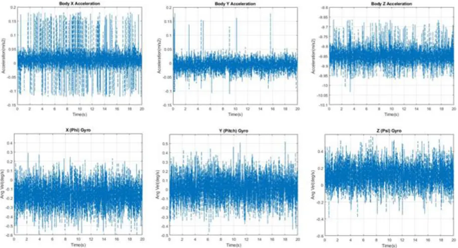
The sensors used in the IMU are a tri-axial accelerometer and a tri-axial gyroscope. Both the sensors are set to sample at the operating frequency of 1 KHz. The inputs to the sensor model are the three axial accelerations and three angular velocities from the plant. First, a transformation of the accelerations in the NED reference frame to the body-reference frame is performed. Gaussian noise is added to the sensor model for these signals after a noise estimation study is conducted. The raw data from the sensors were collected and noise parameters such as mean, variance and the peak-to peak-value of the noise was calculated. Initialization of sensors was performed to remove the bias introduced inherent to the accelerometer and gyroscope sensors. Figure 30 displays the time history responses at a static condition for each sensor signal and are used to quantify the sensor noise and bias characteristics.

62

Data used to calculate the mean values and Vpp of the noise characteristics are shown in Figure 30.

The standard deviation is calculated using the following:

6 𝜎 = 𝑉_𝑝𝑝 (58)

where σ is the noise variance. Table 5 summarizes the sensor noise characteristics.

Table 5: Accelerometer and Gyroscope Noise Estimation Characteristics

Parameters X_Accel (m/s2)

Y_Acce l(m/s2)

Z_Accel (m/s2)

X_Gyro (rad) Y_Gyro (rad) Z_Gyro (rad) Mean 0.02 ~0 -9