A high-order compact integrated-RBF scheme for time-dependent problems

The 4th International Conference on Computational Methods (ICCM2012), Gold Coast, Australia www.ICCM-2012.org

November 25-28, 2012, Gold Coast, Australia www.ICCM-2012.org

A high-order compact integrated-RBF scheme for time-dependent problems

N. Thai-Quang*1, K. Le-Cao1, N. Mai-Duy1, C.-D Tran1 and T. Tran-Cong1 1

Computational Engineering and Science Research Centre, Faculty of Engineering and Surveying The University of Southern Queensland, Toowoomba, Queensland 4350, Australia

*Corresponding author: [email protected]

Abstract

This paper presents a high-order approximation scheme based on compact integrated radial basis function (RBF) stencils and second-order Adams-Bashforth/Crank-Nicolson algorithms for solving time-dependent problems. We employ compact integrated-RBF stencils, where the RBF approximations are locally constructed through integration and expressed in terms of nodal values of the function and its derivatives, to discretise the spatial derivatives in the governing equations. We adopt the Adams-Bashforth and Crank-Nicolson algorithms, which are second-order accurate, to discretise the temporal derivatives. Numerical investigations in several analytic test problems show that the proposed scheme is stable and high-order accurate.

Keywords: time-dependent problems, compact integrated-RBF stencils, high-order approximations Introduction

latter, the information about the governing equation is also included in local approximations to enhance their accuracy.

In this paper, we present a high-order discretisation scheme based on compact integrated-RBF stencils and second-order Adams-Bashforth/Crank-Nicolson algorithms for solving time-dependent problems, where emphasis is placed on the treatment of the extra information in the compact stencils. The proposed scheme is shown to be stable and high-order accurate. The remainder of the paper is organised as follows. Section 2 briefly outlines several time-dependent equations. The proposed compact integrated-RBF scheme is described in Section 3. In Section 4, numerical results are presented and compared with some published solutions, where appropriate. Section 5 concludes the paper.

Problem formulations

In this paper, two types of time-dependent equation, namely a heat equation and the Burgers' equation, are considered.

Heat equation

, 2 2

x u t u

    

, b x

a  t0, (1) u(x,0)u0(x), axb, (2) u(a,t)u1(t) and u(b,t)u2(t), t 0. (3) where u and t are the field variable and time, respectively; and u₀,

1



u and 2



u prescribed functions.

Burgers’ equation

2 2

Re 1

x u x

u u t u

       

, axb, t0, (4) u(x,0)u0(x), axb, (5) u(a,t)u1(t) and u(b,t)u2(t), t 0, (6) where Re0 is the Reynolds number; and u₀(x), ( )

1 t

u_ and ( ) 2 t

u_ prescribed functions. Numerical formulations

Temporal discretisation

Heat equation

The temporal discretisation of (1) with a Crank-Nicolson scheme gives

    

  

              

   

  1

2 2 2

2 1

2

1 n n

n n

x u x

u t

u u

1 2 2 1 2 2 2 2                        n n n n x u t u x u t

u . (8)

Burgers’ equation

The temporal discretisation of (4) with an Adams-Bashforth scheme for the convection term and a Crank-Nicolson scheme for the diffusion term gives

                                            2 1 2 2 2 2 1 1 Re 2 1 2 1 2 3 x u x u x u u x u u t u

un n n n n n

(9) or                                         2 1 2 1 2 1 2 2 2 1 2 3 Re 2 Re 2 n n n n n n x u u x u u t x u t u x u t

u . (10)

Spatial discretisation

Our previous work (Thai-Quang, Le-Cao, Mai-Duy and Tran-Cong, 2012) provided the details of a compact integrated-RBF approximation to the second-order spatial derivatives over a 3-point stencil (Figure 1). Its formulation can be summarised as follows

 

 

 

 

2 3 2 5 2 1 2 4 3

1  

           d u d d d d u d d d u d d d du i i

i  





 (11)

 

 

 

 

2 3 2 2 5 2 2 1 2 2 4 2 3 1 2 2 2 2              d u d d d d u d d d u d d d u d i i

i  







(12) where .

Temporal - spatial discretisation

We consider values of un _{and 2}

2

x un

 

at each node as two independent unknowns. As a result, two algebraic equations need be established at each node.

Consider a node . The first equation is obtained by collocating the governing equation, i.e. (8) in the heat equation and (10) in the Burgers equation, at .

The second equation is derived from (12) for a stencil associated with . Collocating (12) at the central node of a stencil yields

 

 

 

 

2 3 2 2 2 5 2 2 1 2 2 2 4 2 3 1 2 2 2 2 2 2              d u d d d d u d d d u d d d u

d n n n

The present final system of the equations is thus solved for the values of the field variable and its second-order derivative at the interior grid nodes.

Numerical examples

It has been accepted that, among RBFs, the multiquadric (MQ) function tends to result in the most accurate approximation (Franke, 1982). We choose MQ as the basis function in the present calculations

  



2 2

i i

i x x c a

G    (14) wherec_iand a_iare the centre and width of the ith MQ, respectively. For each stencil, the set of nodal points is taken to be the set of MQ centres. We simply choose the MQ width asa_i h_i in which  is a given positive number and h_i the distance between the ith node and its nearest neighbour. The value of  20 is used for all calculations in this paper. We assess the performance of the proposed scheme through the following measures:

(i) the root mean square error (RMS) defined as





N u u RMS

N

i

i i







 1

2

, (15) whereNis the number of nodes over the whole domain and u is the exact solution,

(ii) the convergence rate  with respective to grid refinement defined through NeO

 

h as

   





   





,

/ log

/ log

s r

s r

h h

Ne Ne



 (16) whereh is the grid size; and the superscripts r and sare used to indicate the data obtained from the

r and sth calculations (rs), respectively. Heat equation

By selecting this problem, the performance of the proposed scheme can be investigated for the diffusion term only. Consider equation (1) on the segment [0, π] with the initial and boundary conditions u(x,0)sin(2x), 0x _and u(0,t)u(,t)0, t0 , respectively. The exact solution of this problem can be verified to beu(x,t)sin(2x)e4t.

Firstly, the spatial accuracy of the proposed scheme is tested on various uniform grids



11,21,...101





N . We employ here a small time step, t0.001, to avoid the effect of the approximate error in time. Figure 2 shows the effect of the grid size h on the accuracy of the solution computed at t1, from which one can see that the solution converges as O(h3.4) _{(i.e. of} more than third-order accuracy in space). Figure 3 shows the computed and exact solutions, where good agreement is clearly observed.

Secondly, we test the temporal accuracy of our scheme through a set of time step

   

   

10 1 ,.... 90

1 , 100

1

1



t is shown in Figure 4 as a function of the time stept. It can be seen that our scheme obtains second-order accuracy in time. This result is fully expected as second-order approximation algorithms for the discretisation of time derivative terms are adopted in the present scheme.

Burgers’ equation

This equation involves the convection and diffusion terms. Consider a particular solution, namely shock wave propagation, of Burgers’ equation (4) on the segment 0 ≤ x ≤ 1, t ≥ 0 in the form (Hassanien, Salama, and Hosham, 2005)





,

) exp( 1

) exp( ) (

) ,

( 0 0 0 0



 

  

    

t x

u (17) where ₀Re(x₀t₀), ₀ 0.4, ₀ 0.125, ₀ 0.6, Re100.

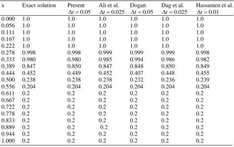
The initial and boundary conditions can be derived from the analytic solution (17). The calculation is carried out at Re100on the grid of N 37. Results obtained are presented in Table 1.The exact solution and some other solutions presented in (Ali, Gardner, and Gardner, 2005; Dogan, 2004; Dag, Irk, and Saka, 2005; Hassanien, Salama, and Hosham, 2005) are also included. It can be seen that the present solution is in good agreement with the other solutions. Figure 5 illustrates the computed solution at different times, which are indistinguishable from the exact solutions.

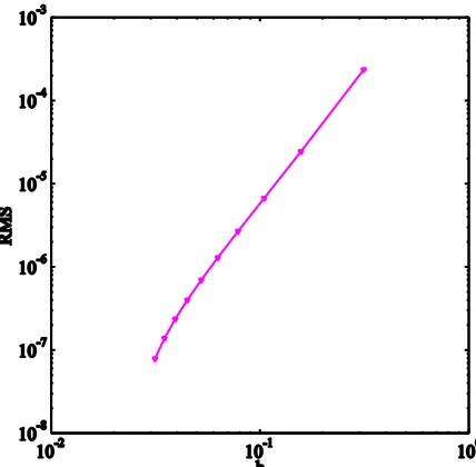
In order to study the convergence of the solution with grid refinement, the calculations are carried out on a set of uniform grids N



11,21,...101



. The time step t is required to be small enough at which the error caused by the temporal discretisation can be negligible. In the present study, the time step t105 is chosen. The errors of the solution against different grid sizes at the time

5 . 0



t are displayed in Figure 6, where the solution converges very fast at a high rate of 4.47. Conclusions

In this paper, a new discretisation scheme for time-dependent problems is presented. The present approximations are based on 3-node stencils, resulting in a sparse system matrix, while Adams-Bashforth/Crank Nicolson algorithms and IRBF-based compact approximations are employed to yield a high-order accurate solution in time and space, respectively. Several test problems are considered to verify the present scheme.

References

Ali, A. H. A.; Gardner, G. A. and Gardner, L. R. T. (2005), A collocation solution for burgers’ equationusing cubic b-spline finite elements. Applied Mathematics and Computation, 170, pp. 781–800.

Bateman, H. (1915), Some recent researches on the motion of fluids. Monthly Weather Review, 43,pp. 163–170.

Caldwell, J.; Wanless, P. and Cook, A. E. (1987), Solution of burgers’ equation for large reynolds numberusing finite elements with moving nodes.Applied Mathematical Modelling, 11(3), pp. 211–214.

Dag, I.; Irk, D. andSaka, B. (2005), A numerical solution of the burgers’ equation using cubic b-splines.Applied

Mathematics and Computation, 163, pp. 199–211.

Dogan, A. (2004), Agalerkin finite element approach to burgers’ equation. Applied Mathematics and Computation, 157, pp. 331–346.

Franke, R. (1982), Scattered data interpolation: Tests of some method. Mathematics of Computation,38, pp. 181–200. Gupta, M. M.; Manohar, R. P. and Stephenson, J. W. (2005), High-order difference schemes for two-dimensional elliptic equations. Numerical Methods for Partial Differential Equations, 1(1), pp.71–80.

Hassanien, I. A.; Salama, A. A. and Hosham, H. A. (2005), Fourth-order finite difference method for solving burgers equation.Applied Mathematics and Computation, 170, pp. 781–800.

Hosseini, B. and Hashemi, R. (2011), Solution of burgers’ equation using a local-rbfmeshless method.International

Iskander, L. and Mohsen, A. (1992), Some numerical experiments on the splitting of burgers’ equation.Numerical Methods for Partial Differential Equations, 8(3), pp. 267–276.

Kansa, E. J. (1990), Multiquadrics- A scattered data approximation scheme with applications to computational fluid-dynamics-I. surface approximations and partial derivative estimates. Computers and Mathematics with Applications, 19(8/9), pp. 127–145.

Kouatchou, J. (2001), Parallel implementation of a high-order implicit collocation method for the heatequation.Mathematics and Computers in Simulation, 54(6), pp. 509–519.

Mai-Duy, N. and Tanner, R. I. (2007), A collocation method based on one-dimensional rbf interpolation scheme for solving pdes. International Journal of Numerical Methods for Heat & Fluid Flow, 17(2), pp. 165–186.

Mai-Duy, N. and Tran-Cong, T. (2001), Numerical solution of differential equations using multiquadricradial basic function networks.Neural Networks, 14, pp. 185–199.

Mai-Duy, N. and Tran-Cong, T. (2011), Compact local integrated-rbf approximations for second-orderelliptic differential problems. Journal of Computational Physics, 230(12), pp. 4772–4794.

Sun, H. and Zhang, J. (2003), A high-order compact boundary value method for solving one-dimensionalheat equations.

Numerical Methods for Partial Differential Equations, 19(6), pp. 846–857.

Thai-Quang, N.; Le-Cao, K.; Mai-Duy, N. and Tran-Cong, T. (2012), A high-order compact local integrated-rbfscheme for steady-state incompressible viscous flows in the primitive variables. CMES: Computer Modeling in Engineering Sciences, 6(2), pp.77–92.

Zhu, C. G. and Wang, R. H. (2009), Numerical solution of burgers’ equation by cubic b-spline quasi-interpolation.

[image:6.595.61.538.397.696.2]

Applied Mathematics and Computation, 208(1), pp. 260–272.

Table 1. Shock wave propagation, grid N=37, Re=100, t=0.5: Comparison between exact and computed solutions

x Exact solution Present Ali et al. Dogan Dag et al. Hassanien et al. t0.05 t 0.025 t 0.05 t 0.025 t0.01

0.000 1.0 1.0 1.0 1.0 1.0 1.0

0.056 1.0 1.0 1.0 1.0 1.0 1.0

0.111 1.0 1.0 1.0 1.0 1.0 1.0

0.167 1.0 1.0 1.0 1.0 1.0 1.0

0.222 1.0 1.0 1.0 1.0 1.0 1.0

0.278 0.998 0.998 0.999 0.999 0.999 0.998

0.333 0.980 0.980 0.985 0.994 0.986 0.982

0.389 0.847 0.850 0.847 0.848 0.850 0.849

0.444 0.452 0.449 0.452 0.407 0.448 0.455

0.500 0.238 0.238 0.238 0.232 0.236 0.239

0.556 0.204 0.204 0.204 0.204 0.204 0.204

0.611 0.2 0.2 0.2 0.2 0.2 0.2

0.667 0.2 0.2 0.2 0.2 0.2 0.2

0.722 0.2 0.2 0.2 0.2 0.2 0.2

0.778 0.2 0.2 0.2 0.2 0.2 0.2

0.833 0.2 0.2 0.2 0.2 0.2 0.2

0.889 0.2 0.2 0.2 0.2 0.2 0.2

0.944 0.2 0.2 0.2 0.2 0.2 0.2

∆t

[image:7.595.191.405.199.409.2]

Figure 1.Compact local 3-point 1D-IRBF stencil

[image:7.595.324.514.502.694.2]

Figure 2. Heat equation, N={11, 21, ...101}, Δt=0.001, t=1: The effect of grid size h on the solution accuracy by the proposed scheme. The solution converges as O(h3.4)

Figure 3. Heat equation, N=101, Δt=0.001, t=1: Variations of the computed and exact

[image:7.595.73.264.509.689.2]

solutions

[image:8.595.79.263.113.300.2]

Figure 5. Shock wave propagation, N=37, Re=100: Profiles of the computed and exact

[image:8.595.323.516.115.307.2]

solutions at different times

Figure 6. Shock wave propagation, N={11,21, ...101}, Re=100, Δt=10-5, t=0.5:

The effect of grid size h on the solution accuracy by the proposed scheme. The