Comparison of optimised composite control charts: improved statistical process control for the manufacturing industry

Full text

(1)ResearchOnline@JCU. This file is part of the following reference:. MacNaughton, David (2008) Comparison of optimised composite control charts: improved statistical process control for the manufacturing industry. Masters (Research) thesis, James Cook University.. Access to this file is available from:. http://researchonline.jcu.edu.au/31904/. The author has certified to JCU that they have made a reasonable effort to gain permission and acknowledge the owner of any third party copyright material included in this document. If you believe that this is not the case, please contact [email protected] and quote http://researchonline.jcu.edu.au/31904/.

(2) Comparison of Optimised Composite Control Charts Improved Statistical Process Control for the Manufacturing Industry. Thesis submitted by David MacNaughton BE(Chem) May, 2008. for the Degree of Master of Science (Research) School of Mathematics, Physics and IT James Cook University.

(3) Statement of Access. I, the undersigned, the author of this thesis, understand that James Cook University will make this thesis available for use within the University Library and, by microfilm or other means, allow access to users in other approved libraries. All users consulting this thesis will have to sign the following statement: In consulting this thesis I agree not to copy or closely paraphrase it in whole or in part without the written consent of the author; and to make proper public written acknowledgement for any assistance which I have obtained from it. Beyond this, I do not wish to place any restriction on access to this thesis.. _____________________________________ (David MacNaughton). ____________ (Date). i.

(4) Statement of Sources. I declare that this thesis is my own work and has not been submitted in any form for another degree or diploma at any university or other institution of tertiary education. Information derived from the published or unpublished work of other has been acknowledged in the text and a list of references is given.. _____________________________________ (David MacNaughton). ____________ (Date). ii.

(5) Statement of Contribution by Others The following list identifies people and institutions which have contributed to this thesis, and the contribution made. •. Professor Danny Coomans – Editing, and Primary Supervision.. •. JCU High Performance Computing Centre (HPC) computing facilities.. •. JCU School of Mathematics, Physics and IT: use of office and associated overheads, supply of personal computer during candidacy, printing, telephone for making contact with industry to obtain data for case studies.. •. Anonymous Referees and the Editor from the Journal of Quality Technology editing for their valuable suggestions.. •. David Cusack of Cement Australia Pty Ltd (CAPL) and CAPL are thanked for provision of industrial data and editing.. I would also like to thank Dr. Yvette Everingham for editing and support.. iii.

(6) Abstract Selecting and configuring control charts can be a difficult task. Literature has not provided evidence as to which type of composite control chart is best among composite moving average (CMA), composite exponentially weighted moving average (CEWMA) and composite cumulative sum (CCUSUM). Optimising three-component composite control charts was considered very difficult, if not impossible, to achieve. Additionally, a traditional method for comparing control charts across a domain of step shift sizes called the average ratio of average time to signal (ARATS), can lead to inconsistent conclusions. Thus, there have been insufficient methods and data published for an informed selection from composite control chart types and configurations. This study is the first to optimise and compare two and three-component composite control charts. Distribution parameters were assumed to be unknown and were estimated from 200 observations. Software was created to automatically configure composite control charts to achieve specifications for the in-control average time to signal (ICATS) and the contribution of each of the components to false alarms, or loadings. Detection time profiles were simulated for full factorial experiments of control chart parameters using averages of at least 1,000,000 chart runs per simulation. New performance and comparison measure were invented to complete the research. A new performance measure Mean Relative Loss (MRL) was defined and used for optimising control chart configurations. MRL compares the average time to signal (ATS) profile across a step shift domain to the profile of a reference CUSUM control chart. Average Difference Relative to the Average (ADRA) was defined to overcome the problem noted with ARATS. Three-component CCUSUM bettered three-component CEWMA (ADRA = 5.0%) which in turn performed better than three-component CMA. Three-component CEWMA performed better than two-component CEWMA (ADRA = 5.2%). Thus it can be seen that the type of component and the number of components selected has a significant effect on performance. This study shows how much the statistical performance of various types of optimised composite control charts can differ. Results from this study will better inform statistical quality control professionals when selecting a control chart type. The methods developed here have the further advantage of being adaptable to different assumptions and parameters. A final implication of the study is that composite control charts may now be optimised and thus fairly compared against other categories of control charts which are typically optimised in literature.. iv.

(7) Table of Contents Statement of Access .........................................................................................................................i Statement of Sources ......................................................................................................................ii Statement of Contribution by Others ......................................................................................... iii Abstract ..........................................................................................................................................iv Table of Contents............................................................................................................................v List of Tables .................................................................................................................................vii List of Figures .................................................................................................................................x Glossary and List of Acronyms ...................................................................................................xii List of Symbols.............................................................................................................................xiv Introduction ....................................................................................................................................1 1.1. Control Charts in Manufacturing ..................................................................................2. 1.2. Rationale for the Study ................................................................................................10. 1.3. Aims of the Thesis ........................................................................................................17. 1.4. Structure of the Thesis .................................................................................................18. Control Chart Definitions and Background Literature ............................................................19 2.1. Process and Process Disturbance Models...................................................................19. 2.2. Formula for Basic Control Charts...............................................................................20. 2.3. Background Literature.................................................................................................25. Performance Measurement and Comparison ............................................................................35 3.1. Comparison and Design of Control Charts .................................................................35. 3.2. Methodology ................................................................................................................39. 3.3. Pair-Wise Comparison Measures for Multiple Disturbance Scenarios.......................40. 3.4.. Individual Scheme Performance Measures for Multiple Disturbance Scenarios ........50. 3. 5. Absolute versus Relative Performance Measures........................................................61. 3. 6. Discussion and Conclusions on Statistical Measures of Control Chart Performance 62. 3.7. Rationale for Defined Assessment Domain Boundaries ..............................................64. Determining Control Chart Properties.......................................................................................67 4.1. Precedence for use of Simulation Software .................................................................67. 4.2. Simulator Overview and Assumptions .........................................................................68. 4.3. Modelling the Contribution of Individual Components ...............................................72. 4.4. Algorithm for Seeking In-Control Specifications.........................................................73. 4.5. Using the Software.......................................................................................................76. 4.6. An Application to Industrial Data ...............................................................................81. v.

(8) 4.7. Concluding Remarks on Significance of the Software .................................................86. Understanding Tuning Parameter Optimisation .......................................................................87 5.1. EWMA Performance over Time...................................................................................88. 5.2. Literature on Comparisons of Basic Control Charts...................................................93. 5.3. MA, EWMA and CUSUM Comparisons ......................................................................93. 5.4. Conclusions on Comparisons Basic Control Charts ...................................................95. Optimisation of Composite Control Charts................................................................................97 6.1. Introduction .................................................................................................................97. 6.2. Methodology ................................................................................................................97. 6.3. Optimised Scheme Configurations...............................................................................99. 6.4. Effect of the Number of Components .........................................................................102. 6.5. Comparison of Three-Component Composite Schemes.............................................104. 6.6. Ramp Location Shift Performance.............................................................................107. 6.7. Hierarchical Monitoring ...........................................................................................108. Conclusions..................................................................................................................................113 7.1. Satisfaction of Thesis Aims ........................................................................................113. 7.2. Interpretations and Limitations .................................................................................117. 7.3. Justification and Significance of the Research ..........................................................119. Recommendations.......................................................................................................................121 8.1. Optimisation for Alternative Assumptions .................................................................122. 8.2. Monitoring Needs within an Organisation ................................................................123. 8.3. Form of CCUSUM Presentation................................................................................124. 8.4. Identification and Correction Tools...........................................................................124. 8.5. Composite Control Charts for Multivariate Techniques ...........................................124. Appendices ..................................................................................................................................125 Appendix A - Error Analysis ....................................................................................................126 Appendix B - MA and EWMA ATS Profiles .............................................................................129 Appendix C - Composite Scheme Design Dataset....................................................................133 Appendix D - Validation of the Software .................................................................................134 Appendix E - Software Details .................................................................................................139 Appendix F - Comparison of Designs for Different Assessment Domains...............................143 Appendix G - Four-Component CEWMA Designs for Various ICATS Targets.......................145 References....................................................................................................................................147. vi.

(9) List of Tables Page 3-1.. Demonstration of ARSSATS calculation for designs by Wu and Wang (2007).. 42. 3-2.. Example of a problem with MRLPC: MA(2) versus MA(3).. 45. 3-3.. Fictitious example of two comparable schemes.. 46. 3-4.. SSATS values derived for CCUSUM3D for known parameters.. 49. 3-5.. CCUSUM3B and various run rules schemes by Koo and Ariffin (2006) using the MRLMC performance measure.. 3-6.. 53. Optimum CUSUM reference vector, OCV, used for RLOCV calculations. The vector was created from profiles of 15 different CUSUM schemes.. 57. 3-7.. CUSUM reference scheme, Cδ , used for RL calculations.. 58. 3-8.. MRL and RLE performance for optimum MA(n) schemes.. 58. 3-9.. Experimental design levels for two-component CCUSUM scheme optimisation.. 3-10.. 60. MRL and MRLOCV performance for two-component CCUSUM schemes at Al1IC = 25% slice of the experimental lattice.. 60. 4-1.. Compressive Mortar Strength Dataset Statistics.. 81. 4-2.. Control Chart Design Convergence Results.. 84. 4-3.. Composite Control Chart Design CCUSUM4a for 28-day Compressive Mortar Strength (Cement Quality) Example.. 5-1.. Comparison of optimised MA control charts relative to optimised EWMA control charts.. 5-2.. 85. 94. Comparison of optimised CUSUM control charts relative to optimised EWMA control charts.. 95. vii.

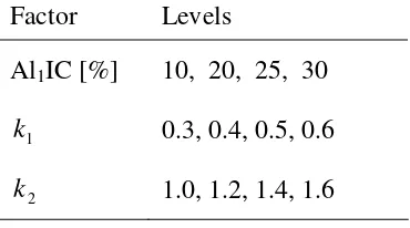
(10) 6-1.. Levels used in optimisation of the CEWMA2, CMA3, CEWMA3 and CCUSUM3 schemes. Al j IC% refers to the percentage of alarms attributable to component j when the monitored variable is in an incontrol state.. 98. 6-2.. Configuration and performance of optimized composite schemes.. 99. 6-3.. Error bars for simulated MRL results.. 6-4.. Comparison of optimized three-component composite schemes on ramp. 103. location shifts relative to the CCUSUM3 scheme.. 107. A-1.. CMA3 Error Analysis.. 126. A.2.. CEWMA3 Error Analysis.. 127. A-3.. CCUSUM3 Error Analysis.. 128. B-1.. ATS profiles and MRLMC comparison of MA control charts for a selection of designs from MA(1) to MA(30).. B-2.. 130. ATS profiles and MRLMC comparison of EWMA control charts for a selection of designs from EWMA(0.02) to EWMA(1).. 131. C-1.. Scope of composite control chart design and performance dataset.. 133. D-1.. Validation of EWMA ATS on known parameters by comparsion against Lucas and Saccucci (1990).. D-2.. 135. Validation of CMA step and ramp ATSs on known parameters by comparsion against Plan 5 (Sparks, 2003).. D-3.. Validation of two sided CUSUM ATSs on known parameters by comparsion against Sparks (2000).. D-4.. 136. 137. Validation of estimated parameters results for individuals Shewhart Chart ATSs with nestim = 100, by comparsion against Quesenberry (1993).. D-5.. 137. Validation of normally distributed data created using the C++ class StochasticLib class (Fog, 2003) which is based on the Mersenne Twister algorithm.. 138. viii.

(11) F-1.. G-1.. Comparison of Sparks’ CCUSUM3 scheme relative to the optimum CCUSUM3 scheme.. 143. Designs for CEWMA4 schemes with ICATS = 100 to 1000.. 145. ix.

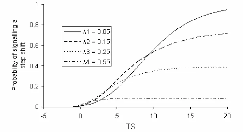
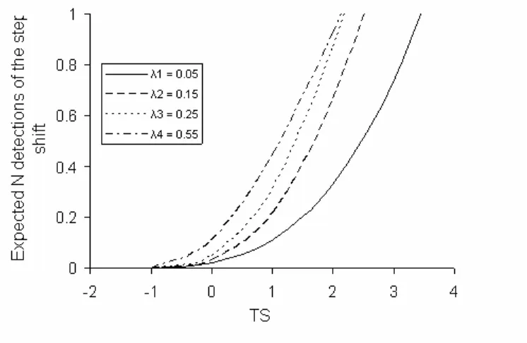
(12) List of Figures 1-1.. Pie chart of contribution by industry to gross domestic product in. Page. Australia, 2002. Source: Queensland state government web page https://www.qld.gov.au. 1-2.. 3. Appearance of a simple control chart. Normal curve added to demonstrate the distribution of the data.. 5. 1-3.. The cycle of process monitoring and correction.. 7. 1-4.. Compressive mortar strength history courtesy of Cement Australia Ltd (Un-named production site and manufacturing period).. 9. 3-1.. Augmented process monitoring and correction cycle.. 36. 3-2.. Woodall (1985)’s control regions.. 38. 3-3.. Control regions used results for scheme designs in Section 3.3 and 3.4.. 40. 3-4.. SSATS profiles of Moving Average Control Charts, MA(2) and MA(3).. 44. 3-5.. RLMC profiles for EWMA(λ) type schemes where λ is defined in the legend and CEWMA4D is defined by the design [λ1 = 0.055, h1 = 2.9849; λ2 = 0.3, h2 = 3.2286; λ3 = 0.55, h3 = 3.2841; λ4 = 1.0, h4 = 3.3259].. 4-1.. 55. The graphical user interface of the simulator software created for the thesis.. 69. 4-2.. Flow chart for the simulation of ATS values from ntrials x chart runs.. 71. 4-3.. Dialog box for defining a three- to four-level full factorial CCUSUM3 performance measurement experiment.. 4-4.. 78. Cement 28-day compressive mortar strength data provided by Cement Australia Pty. Ltd. Unnamed production facility and manufacturing period.. 5-1.. 86. The probability of detecting a step shift using EWMA schemes with λ = 0.05 to 0.55, for a step shift of 1 σ , ICARL = 400 observations, based on 100,000 simulated chart runs.. 89. x.

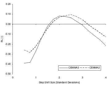
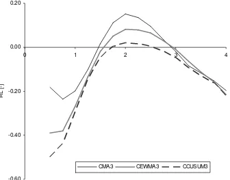
(13) 5-2.. The probability of detecting a step shift using EWMA schemes with λ = 0.05 to 0.55. for a step shift of 2 σ with ICARL = 400 observations, based on 100,000 simulated chart runs.. 5-3.. 89. The expected number of alarms for detecting a step shift of 1 σ using EWMA schemes with λ = 0.05 to 0.55, with ICARL = 400 observations, based on 100,000 simulated chart runs.. 5-4.. 91. The expected number of alarms for detecting a step shift of 2 σ using EWMA schemes with λ = 0.05 to 0.55, with ICARL = 400 observations, based on 100,000 simulated chart runs.. 5-5.. 91. Optimal ATS for the CUSUM Control Chart for Step Shift of 0.5 , with ICATS = 400.. 94. 6-1.. Surface plot of MRL values for CEWMA2 designs, Al1 % = 45% .. 100. 6-2.. Surface plot of MRL values for CEWMA3 designs. λ2 = 0.43,. λ3 = 0.96, Al2 IC % : Al3 IC % = 55 : 45 . 6-3.. Surface plot of MRL values for CMA3 designs. n2 = 2, n3 = 1, Al2 IC % : Al3 IC % = 50 : 50 .. 6-4.. 102. RL profiles for optimum CMA3, CEWMA3 and CCUSUM3 control charts, relative to the reference CUSUM scheme (k=1.1, h=2.2908).. 6-7.. 101. The RL profile of optimum CEWMA2 and CEWMA3 schemes, relative to the reference CUSUM scheme (k = 1.1, h = 2.2908).. 6-6.. 101. Surface plot of MRL values for CCUSUM3 designs. k2 = 1.0, k3 = 1.8, Al2 IC % : Al3 IC % = 50 : 50 .. 6-5.. 100. 105. Simplified organisational chart showing the process and laboratory components for a large manufacturing plant operation.. 108. E-1.. Specification seeking algorithm.. 139. E-2.. C++ class inheritance structure.. 142. F-1.. ATS profiles for CCUSUM3a and a CCUSUM3 scheme by Sparks (2000).. 144. xi.

(14) Glossary and List of Acronyms ACUSUM. Adaptive Cumulative Sum technique for control chart design. AEWMA. Adaptive EWMA technique for control chart design. ADRA. Average Difference Relative to the Average. ARARL. Average Ratio of Average Run Length. ARL. Zero-State Average Run Length. ARSSATS. Average Ratio of Steady State Average Time to Signal. ATS. Zero-State Average Time to Signal. This is equivalent to the Average Time to Signal by other authors.. CAPL. Cement Australia Pty. Ltd.. CEWMA. Composite Exponentially Weighted Moving Average. CMA. Composite Moving Average. CUSUM. Cumulative Sum. DCS. Distributed Control System. DRA. Difference Relative to the Average. EWMA. Exponentially Weighted Moving Average. Component. A component of a composite control chart scheme, i.e. one chart from a group of control charts monitoring the same quality variable, which are designed to have joint in-control specifications. FIR. Fast Initial Response. ICARL. In-Control Average Run Length. ICATS. In-Control Average Time to Signal. iid. Independently and Identically Distributed. ISO. International Standards Organisation. LCL. Lower Confidence Limit. Loading. The proportion of alarms contributed by a specific component when the monitored variable is in-control. LIMS. Laboratory Information Management System. MA. Moving Average. MRL. Mean Relative Loss. xii.

(15) MRLMC. Mean Relative Loss Multiple Comparison. MRLPC. Mean Relative Loss Pair-Wise Comparison. MRLOCV. Mean Relative Loss to the Optimum CUSUM Vector. PC1. Principle Component - Number 1. PCA. Principle Components Analysis. PIMS. Process Information Management System. RAEQL. Ratio of Average Extra Quadratic Loss. RLE. Relative Loss Efficiency.. RLPC. Relative Loss Pair-Wise Comparison. Run Rules. Conditions for which a control chart is required to alarm such as two consecutive samples being outside of a corresponding set of control limits.. Scheme. Control chart or group of control charts. SPC. Statistical Process Control. SPSS. Trademark of the statistical software used for the data processing.. SS. Steady State. SSATS. Steady-State Average Time to Signal. SSARL. Steady-State Average Run Length. TS. Time to Signal. UCL. Upper Confidence Limit. X-Chart. An individuals control chart; equivalent to a Shewhart chart when the control limit coefficient, h, equals 3.0. X -Chart. Xbar control chart; a scheme which monitors the average of groups of data with a defined number of sequential samples. X -EWMA. A hybrid control charting technique comprising of Xbar and EWMA components with separate control limits for each component. X -CUSUM. A hybrid control charting technique comprising of Xbar and CUSUM components with separate control limits for each component. X-MR. Individuals – Moving Range composite control chart. xiii.

(16) List of Symbols AlIC. Vector of component loadings (percentage contributions by each component in a composite scheme to the gross false alarm frequency). AlIC Target Alγ IC. Loadings (percentage contributions by each component in a composite scheme to the gross false alarm frequency) for component. γ c1. Intercept of the secant which relates the ICATS to the ICATS search dimension variable, l. c3. Vector of intercepts of the secants which relate the loadings, AlIC , to the vector loadings search dimension variables, g. δµ. Parameter for step shift in the location of the mean, normalised. δσ. Parameter for step shift in the standard deviation, coefficient. εi. Random error component of a signal, at iteration i. g. Vector of component loading search dimension variables. h. Vector of control limit coefficients. hj. Control limit coefficient for component j when distribution parameters are known. hj ’. Control limit coefficient for component j when distribution parameters are estimated from a sample of size nestim. k. Reference parameter for CUSUM charts. κ. Ramp rate coefficient. l. ICATS search dimension variable. λ. Weighting parameter for EWMA charts. m1i. The gradient for the SSATS search dimension variable li calculated for iteration i. m3i , j. Gradients for the component loading search dimension variables gi , j for search iteration i. MR. Absolute value of the moving range. xiv.

(17) MA j. Moving average statistic for component j. µ0. Mean of the in-control reference population. n. Span parameter for MA charts. nδ. Number of nodes, location shifts at which control chart schemes are compared. neffective. The span which would characterise a MA control chart which would have a power similar to the EWMA control chart under consideration. nestim. Number of observations used to estimate the parameters of a variable. ntrials. Number of chart runs used in the simulation of an ICATS value. P. A control chart parameter such as λ for EWMA charts, k for CUSUM charts, and n for MA charts. s. Standard deviation estimated via the mean sum of squares based formula. σ. Altered standard deviation of monitored variable. σ0. Standard deviation of the in-control reference population. σQ. Standard deviation of the EWMA statistic. t. Estimated mean from a sample of in-control observations. τ. Observation number. Yi. Value of the monitored variable at observation i. wi. Response vector from a simulation. Contains the elements [ICATS, Al1IC, Al2IC, …., AlvIC]. xv.

(18) Chapter 1 – Introduction. Chapter 1. Introduction Statistical process control is a field primarily researched from the perspective of two different schools: industrial engineering and business. Control charts, the subject of this thesis, are a subset of statistical process control tools used for monitoring for deviation from a stochastic model over time.. Potential. applications for control charts are monitoring indicators of asset utilisation, agriculture, environment, macro-economics, community health and welfare, but control charts are most commonly applied in process and laboratory quality control within the manufacturing industry. A major consideration for choosing the type of control chart to use for an application is detection performance. Many different control chart types have been defined since 1924 including: univariate and multivariate; individual, X , simple moving average (MA), exponentially weighted moving average (EWMA), cumulative sum (CUSUM) and run rules (Montgomery, ). Control chart selection and design may present a daunting set of considerations for a person wishing to implement an optimised system of control charts. Composite control charts, which offer good performance for a range of location shifts (Sparks, 2000), have insufficient comparisons available in literature to aid an informed selection. More detection power is still needed in some applications, particularly where costly offline analysis is concerned. Methods for limiting false alarms are also required in data rich environments. This thesis makes a contribution to both of these areas. Schemes comprising of multiple cooperating control charts monitoring a single variable are sometimes called composite control charts. Alternatively they may be called composite monitoring schemes. Composite control charts based on MA, EWMA, and CUSUM control charts have been noted (Lucas and Saccucci, 1990; Sparks, 2000, 2003; Klein, 1996, 1997) to offer good performance over a range of location shift sizes. In this thesis, composite schemes are denoted by adding “C”. 1.

(19) Chapter 1 – Introduction. as a prefix to the abbreviation of the basic statistic, eg. CMA is the abbreviation for composite moving average. The primary aim of this thesis was to compare the statistical performance of CMA, CEWMA, and CCUSUM control charts for the first time over a range of location shift sizes to provide sufficient insight for informed selection from control chart options. The features of composite control charts which may facilitate use within a management structure were also explored.. 1.1. Control Charts in Manufacturing. 1.1.1. Australian Manufacturing Context and Motivation. In 2002, manufacturing activity represented a contribution of 13.3% to Australia’s gross domestic product and a similar percentage of employment within Australia; whilst the contribution to export earnings was 47.3% (see Figure 1-1). Cost of production typically decreases as technology develops through innovations. Innovations are arguably driven by competition.. Sustaining the level of. Australian exports income, clearly important to maintaining the gross domestic product, requires Australians to innovate.. Innovations in statistical process. control may make a small contribution to the competitiveness of manufacturing and other industries in the years to come. Benefits could include increased energy efficiency via stabilised process plant operation and improved product quality. Some shortcomings in control chart technology, as noted in Section 1.2, have provided opportunities for novel and innovative works in this thesis.. 2.

(20) Chapter 1 – Introduction. Figure 1-1. Pie chart of contribution by industry to gross domestic product in Australia,. 2002.. Source:. Queensland. state. government. web. page. https://www.qld.gov.au. Please note that cement and mineral processing businesses, interest areas of the author, are grouped within the category of Manufacturing by the Australian Bureau of Statistics. Cement industry data are used as an example later in this thesis.. 1.1.2. Trends and Opportunities for Statistical Process Control. Monitoring algorithms needed to be simple for the most part of the twentieth century because updating calculations and plotting of a control chart was labour intensive. Technology currently used in industry is considerably more advanced than that which was available upon the invention of the Shewhart chart in 1924 (Shewhart, 1931). Measurement, analysis and charting of process variables are mostly automated in. recently commissioned continuous-process. plants.. Distributed control system (DCS) software is used to manage many modern process plant operations where streams of individual measurements are collected. Premium level process information management system (PIMS) software includes Matrikon’s ProcessMonitor™, ProcessDoctor™ (Matricon Pty. Ltd., 2004), and Honeywell’s Experion PKS (Honeywell Pty. Ltd., 2004).. 3. PIMS.

(21) Chapter 1 – Introduction. software are designed to access databases written by the DCS software. Features of modern PIMS software now include advanced statistical process control algorithms including multivariate projection methods such as partial least squares and principle component analysis. This advancement provides an opportunity for adoption of more complex statistical process control algorithms.. 1.1.3. Purpose and Architecture of Control Charts. Control charts are used to detect changes in the distribution of a variable over time, effectively by performing serial statistical inference tests. Therefore, control charts have statistical properties conditioned to specified assumptions. Control charts differ from classical data analysis in which experimental data are analysed at the end of each screening stage. When collecting data from a continuous process plant, one may wish to detect a change in the mean of a variable as fast as possible. An inference test is needed upon every instance that a new item of data becomes available. Constructing an individuals control chart (X-Chart) involves plotting a line-chart of the variable and marking the position of the assumed mean of the data (see Figure 1-2). Control limits are then plotted. A control limit is a boundary at which an alarm is signalled indicating a change in the local mean of the variable. For normally distributed variables the upper control limit (UCL) and lower control limit (LCL) are symmetrical about the assumed mean of the data. A simple design approach requires specifying the in-control average run length (ICARL) and then determining the required offset for the control limits from the mean to achieve that ICARL. The default design value for the margin for the control limits about the mean was historically three standard deviations (Shewhart, 1931; Nelson, 1982) giving an ICARL of 370.4. When an assay falls outside of the range between the control limits, investigation into the cause of the deviation should then commence. More elaborate control chart configurations and design procedures are discussed later.. 4.

(22) Chapter 1 – Introduction. Figure 1-2. Appearance of a simple control chart. Normal curve added to demonstrate the distribution of the data. Adapted from image supplied by Six-Sigma First (2007).. 1.1.4. Control Chart Use. Having knowledge of a shift in process values is useful because it provides the operator with a flag to search for, and to correct, the cause of the process shift. Removing the cause of the process disturbance may remove any corresponding threats to equipment longevity, plant productivity and product quality that were introduced by the process disturbance. Control charts are usually configured in a way that they alarm upon: detection of a shift in the local mean (location) of a variable; an increase in the variance, and Type I inference errors. This thesis focuses on measuring and optimising the performance of control charts for detection of shifts in the location of a variable’s mean. A Type I inference error occurs when it is concluded that a new sample is not from the population being considered when it actually is from that population (Walpole and Myres, 1989). Control charts are intended to alarm for actual changes in the distribution of a variable related to “assignable” causes. Incidental alarms related to Type I errors are not desired, but are inevitable nevertheless. Some control charts also exist for detecting a reduction in variance (MacGregor and Harris, 1993; Braun, 2003). Alarms related to Type I inference error may be considered, in practical terms, as an event where an unlikely combination of “common causes” coincide. For a. 5.

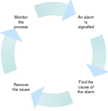
(23) Chapter 1 – Introduction. more detailed explanation, please refer to Montgomery and Woodall (1997). Frequently called “false alarms”, breaches of the control limits related to Type I errors often return to a non-alarm state within a few observations.. Common. cause variation is accepted as part of an in-control process. Interacting with product specifications, common cause variation affects the process “capability” (Wang et al, 2000; Veevers, 1998), and may include considerable random sampling error.. Common causes are usually addressed through continuous. improvement programs, which may require capital investment or development of new technologies. Assignable causes are related to discrete failures that may be addressed immediately in a narrow project scope.. False alarms should be. minimised so that one’s confidence in the control chart, hence one’s alertness to assignable causes, is maintained. Reducing common cause variation requires improvement of the process and may require significant capital to purchase newer technologies. Alternatively, significant operating expenditure may be required to change of a number of operating procedures, changes which are typically based on much data and managed in a planned and non-reactive manner. Another reason that excessive false alarms are not desired is because of the overadjustment phenomenon (see Nelson, 2003). A control chart may not instantly alarm the effect of an assignable cause after onset.. The design of a control chart can minimize detection times with. consideration to an acceptable false alarm rate. In a small fraction of cases, assignable causes may be quickly rectified by virtue of a feedback mechanism, or even by accident. Assignable causes that disappear after one observation have been called isolated special causes (Hawkins et al, 2003).. Conversely, there are sustained assignable causes for which an. investigation must be carried out to identify the cause of the location shift and the most appropriate way to rectify the situation.. Figure 1-3 is a simplified. description of the cycle of activities in which control charts play part with the intention of keeping a process predominantly in-control.. 6.

(24) Chapter 1 – Introduction. Monitor the process. An alarm is signalled. Remove the cause. Find the cause of the alarm. Figure 1-3. The cycle of process monitoring and correction. Plant operators and engineers may be required, by a company’s quality policy, to act upon alarms generated by control charts. In reacting to an alarm, it is best to firstly diagnose the cause of the location shift using experience and operating records. Once a diagnosis is arrived at, a decision may be made to initiate restoration activities immediately. Alternatively, it may be decided to wait a period of time for a suitable maintenance window before correcting the apparent process problem. Upon restoration of the apparent cause, it might be discovered that the diagnosis was incorrect, and so the process of fault finding and restoration must be repeated. It can been seen that the total amount of time in which the process is not performing as intended is from the onset of the location shift until removal of the process shift. There are many components of time that make up this period of off-target production. Given below is a hypothetical quality control example based on 6 hourly off-line analysis. An expanded list of the sequential activities, and corresponding time intervals that occur after a serious quality problem becomes evident, may include:. 7.

(25) Chapter 1 – Introduction. •. Location shift in variable. Interval between this event and sampling may be some part of 6 hours, say 3 hours.. •. Sample transfer laboratory or offline analyser ~ 10 minutes. •. Analysis of sample ~ 15 minutes. •. Data transfer/entry into the control chart ~ 10 seconds. •. Control chart Time to Signal (TS): from first location shifted data entry to detection ~ some multiple of 6hours, eg, 0, 6, 12, …hours. •. Alarm signal to be noted by an Operator and commencement of action ~ 10 seconds to 20 minutes depending on other priorities. •. Root cause analysis ~ 10 minutes to 2 weeks. •. Management involvement and waiting time until maintenance opportunity ~ 0 seconds to 6 months.. •. Engineering and operations activities to rectify the problem ~ 1 hour to 10 days.. Selection of a control chart design typically falls under the accountability of a quality manager. The basis of the control chart selection by a quality manager may consider set-up and operational cost, the efficiency in detecting excursions in quality, presentation and user friendliness.. 1.1.5. Introducing Cement Quality Variables. Cement is a synthetic ingredient that is used in concrete and other building materials and is made from ground clinker, limestone and gypsum; used extensively in housing, civil structures and increasingly in roads. One measure of cement quality is the compressive strength it develops in a mortar form, a mixture of cement, sand and water. The International Organization for Standards (1989) provides a procedure for testing mortar compressive strength.. Mortar. compressive strength displays high variance between homogenous “control samples”, having a standard deviation between 0.6 MPa and 1 MPa depending on the laboratory. Other important performance measures of mortar include the. 8.

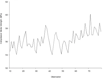
(26) Chapter 1 – Introduction. Blaine (cm2/gram), false set (mm), initial set (hr), final set (hr), normal consistency (mm), and 3, 7 and 28 day concrete strengths (MPa). Typical factors affecting the mortar compressive strength include the chemical and mineral composition of the raw materials, the ratio to which they are mixed, and the particle size distribution of the ground product. Cement Australia Pty Ltd (CAPL) provided data for use in this thesis. Figure 1-4 shows some compressive mortar strength (“ISO” as it is often referred to informally) history depicting a positive step or ramp shift at Observation 64. Compressive mortar strength sometimes increases due to increasing recirculating load in closed-circuit milling process. Control charts are applied to these data in a later chapter.. Compressive Mortar Strength (MPa). 62. 60. 58. 56. 54. 52 10. 20. 30. 40. 50. 60. 70. Observation. Figure 1-4. Compressive mortar strength history courtesy of Cement Australia Ltd (un-named production site and manufacturing period).. 9.

(27) Chapter 1 – Introduction. In 2003, Cement Australia’s quality assurance approach was monitoring individual data using fixed width control limits arranged in warning and action zones.. 1.2. Rationale for the Study. From literature, it is unclear what type of composite control chart offers the best statistical performance for a distribution of step shifts. The rationale behind this thesis relates to weaknesses in existing control chart performance measures, opportunities for optimisation of composite schemes, and developments required for making control charts designs scalable for use on a large number of variables. Listed in point form, the research is intended to cover the following knowledge base gaps: •. Some traditional assumptions in control chart studies are not representative of a typical manufacturing application.. •. Few publications have used a scalar statistical measure to describe the performance of a control chart over a number of location shifts scenarios.. •. Existing scalar statistical measures for control chart performance, over a number of location shifts, do not give values that are readily cross referenced between publications.. •. Composite schemes have not previously been statistically optimised and compared. The effects of the type of composite scheme selected, and the number of components in a composite scheme, are not known.. •. No method has been described which facilitates scaling of control chart designs according to the number of variables to be monitored by each level of company management.. Factors which made the timing of the thesis favourable include: •. Advances in computational processing rates. •. Proliferation of SPC complementary software in industry. The points of rationale are expanded in the following subsections.. 10.

(28) Chapter 1 – Introduction. 1.2.1. Existing Performance Measures and Comparison Techniques. A description of control chart performance over a breadth of location shifts has mostly relied on verbal descriptions and graphs (eg. Jones, Champ and Rigdon, 2001) as opposed to use of a scalar statistical measure (eg. Sparks, 2003). Often performance is described by stating the ARL for one specific location shift, for example, the ARL for a one standard deviation shift in the mean. In reality, assignable causes occur with a distribution of location shifts sizes. A standardised measure of chart performance over a distribution of location shifts is needed so that users can make a well informed design selection. To optimise control charts for a distribution of location shifts, a scalar value is required to represent the expected long-term performance.. Sparks (2003) developed a performance. comparison measure for a domain of step and ramp location shifts which he called relative loss efficiency (RLE). Whilst this is an important advance for control chart studies, RLE is not very suitable for use in an optimisation routine. A new statistical performance measure is required to succinctly compare control charts over a domain of step shift sizes, having a value which is readily transportable for making comparisons between publications, and which can be used for optimisation.. 1.2.2. Optimised Composite Scheme Comparison. There is a gap in the knowledge base of optimum CMA, CEWMA and CCUSUM scheme performance: none of these schemes have been statistically optimised. See, for example: Sparks, 2003, on CMA; Klein, 1996, on CEWMA; Sparks, 2000, on CCUSUM; Sparks (2004) on Group of Weighted Moving Averages. In each of the publications above, a few seemingly ad-hoc designs are compared. Therefore, it is not known how much these schemes differ in performance when optimised. Sparks (2003) compared a number of CMA schemes against EWMA and CUSUM schemes and found that the CMA scheme demonstrated fast detection for a range of location shifts. It cannot be expected that these apparently ad hoc 11.

(29) Chapter 1 – Introduction. (or semi-optimised) design results will necessarily be optimum for the domain of location shift considered. He noted that CMA schemes were favourable from the point of view that the MA statistic may be simpler to understand for less statistically trained SPC users than the CUSUM statistic. Due to the lack of local or global optimisation, further consideration of CMA schemes is warranted. Hence CMA schemes have been included in comparisons of this thesis. CEWMA schemes with two components have been investigated by Albin, Kang and Shea (1997) who noted that CEWMA charts can detect increases in variance with favourable ICARL values. They showed the reduction in ICARL was less for an X -EWMA composite than for the X and Moving Range ( X -MR) composite, but detection of large (factors greater than 2) step shifts in the standard deviation were detected similarly as fast. Therefore, optimised CEWMA schemes could potentially make range charts redundant. Roberts (1959) suggested that, given any MA control chart, an EWMA control chart can be constructed with roughly equivalent properties. Therefore, it might also be expected that CMA and CEWMA control charts will also perform similarly when optimised. Sparks (2003) claimed that he trialled unspecified three-component CEWMA schemes which reportedly did not perform as well as CMA designs. He recommended further development of CEWMA schemes as the initial attempts were unlikely to produce an optimal design. EWMA control charts have been found to perform well in detecting ramped location shifts (Sparks 2003).. CEWMA schemes, which are based on several EWMA. components, may also retain this strength and similarly be efficient at trend detection. CEWMA schemes may have strengths other than performance on step location shifts that have not previously been considered. CEWMA schemes were included in the thesis to expand the knowledge base on this tool. Finally, let us consider the potential value of optimising CCUSUM schemes. Lucas and Saccucci (1990) showed that CUSUM and EWMA schemes perform similarly, concluding that practical issues be used to decide which scheme to select.. Therefore, it is reasonable to expect that CCUSUM and CEWMA. 12.

(30) Chapter 1 – Introduction. schemes will also perform similarly.. Hence, CCUSUM schemes were also. included in the thesis. In summary, CMA, CEWMA and CCUSUM, are all expected to perform similarly based on extrapolation of simpler concepts from literature.. Some. features differentiating MA, EWMA and CUSUM techniques, other than statistical or economic performance measures, have also been noted in literature. It is acknowledged that consideration of these features may assist in selection of a control chart.. However, to date, no quantitative performance data based on. optimisation and comparison of composite schemes has been published. Comparison of optimised composite monitoring schemes will remove all ambiguity related to the statistical performance of various composite schemes from the selection process. Possessing such information, users will be better informed on the general properties of composite schemes. This work is not intended as a substitute for detailed investigations such as economically optimising total quality cost.. 1.2.3. Advances in Computational Processing Rates. Control chart properties can be derived or simulated.. Simulation has been. popular over a long period of time and has been used by authors such as Albin Kang and Shea (1997), Klein (1996, 1997), Jiang, Wu, Tsung, Nair and Tsui (2002), Sparks (2003), and Reynolds and Stoumbos (2004). Simulation provides a simple way of determining control chart properties, particularly in the case of composite schemes which can be complex to derive analytically. Simulation, however, does not lead to exact determination of control chart properties. The properties are estimated from a sample; therefore, a confidence region exists about each estimate.. Advances in computer processing rates have permitted. increased simulation sample sizes for a given processing time. Large sample size simulations were used in this thesis to distinguish control charts which have similar performance.. 13.

(31) Chapter 1 – Introduction. Decreased simulation costs has also meant that full factorial experimental designs have become feasible for investigating optimum composite designs.. The. advantage of optimising via full factorial designs, over advanced methods like genetic algorithms, is the option to create educational surface area plots for inclusion in the research results. One can also investigate interactions between the design parameters. Composite control charts researched in this thesis required up to four times as many computations than do single component control charts. Advances in computer processing rates have increased the feasibility of research into control charts which are computationally demanding to research. Not only can affordable modern personal computers be used to research composite schemes, they are capable of updating and plotting the increased number of signals in a manufacturing plant which may have thousands of raw variables (being a mixture of on-line and off-line measurements). 1.2.4. Proliferation of SPC Complementary Software. Process information management system (PIMS) databases and performance management software are standard inclusions in new processing plants and a significant fraction of older plants have implemented such systems. Performance management software (see examples in Section 1.2.2) makes it easy to build control charts and the real-time computations are automatic. It is estimated that it would be economically feasible to create control charts for all controlled variables within a manufacturing company where previously only key quality variables were typically monitored in this way. Adoption of published control chart technology by industry has been poor (Woodall and Montgomery, 1999).. Poor adoption suggests that there are. outstanding issues for implementation and operation of complex control charts, or lack of awareness of the availability of these techniques. There have been many innovations in the control chart field, particularly since 1980, with some very complex, and powerful tools developed. Public debate over the reasons for poor adoption, and what might be done to increase adoption, arises periodically in the 14.

(32) Chapter 1 – Introduction. Journal of Quality Technology (for example Woodall and Montgomery, 1999; Montgomery and Woodall, 1997). Suggested reasons for poor adoption include the fact that users of control charts have very little statistical training; and some publications have purely academic merit and were never intended to be directly used in applications but are valued because they lead to more practical concepts. One particular design issue that has not been mentioned, is scaling control chart designs for process plants with vastly differing numbers of variables to be monitored. Industry began to centrally collect data at a high frequency for a large number of variables with the adoption of DCSs from around the early 1990s. Each control chart being operated has a certain false alarm rate. An increased number of monitored control charts incur a proportional increase in the total false alarm rate. An overload of false alarms could develop if all quality variables are monitored using control charts. Personnel involved in root cause analyses of assignable causes may learn that no assignable causes exist for some alarms. Reduced motivation to rigorously investigate further alarms may then result. Control charts may be used to generate exception reports. A large number of control charts present a logistical challenge to monitoring of quality by middle levels of management. The configuration of composite schemes may provide an opportunity to address the problem of scaling control chart designs for monitoring at different levels within a company hierarchy. Such an innovation would be a contribution to resolving practical issues experienced by industry; an issue which might otherwise cause resistance to adoption of control charts for plant-wide implementation.. 15.

(33) Chapter 1 – Introduction. 1.2.5. Traditional Assumptions in Control Chart Studies. A review thesis by Woodall and Montgomery (1999) recommended that future research includes techniques for data rich and multi-step processing environments, data reduction methods, economic designs and study of the effect of estimated parameters, etc. On the subject of the effect of estimated parameters they said: “Much more research is needed in this area recognising that Phase II control limits are in fact, random variables. Research shows that more data than has been traditionally recommended is needed to accurately determine control chart limits.” The distribution parameters of monitored variables are not known in practice and must instead be estimated. Comparison of composite control charts by Sparks (2000, 2003) assumed known parameters, as have many publications.. An. assumption of known parameters does not reflect the situation of a typical company where control charts are applied. Conclusions regarding control chart alarm profiles for known parameters may not necessarily be consistent with an assumption of unknown parameters.. No research has been published for. composite control charts with estimated parameters, so it is unclear what type of composite control chart will perform best in real situations. Studies into the comparative performance of CMA, CEWMA and CCUSUM schemes based on estimated parameters have not previously been published. Optimising and comparing composite schemes in simulations where parameters are estimated is the approach used in this thesis.. 16.

(34) Chapter 1 – Introduction. 1.3. Aims of the Thesis. The basic objective of this thesis was to explore composite control charts so that manufacturing end users would be sufficiently informed to select a suitable control chart. The control charts to be explored were CMA, CEWMA, and CCUSUM. The primary aim was: Aim 1 - understand which of these composite control charts performed best over a domain of location shift sizes. Specifically, the statistical performance was sought based on appropriate assumptions for typical manufacturing end users. That is to say, distribution parameters should be estimated rather than assumed to be known. To achieve the primary aim, the following tasks were essential: •. Develop improved statistical measures and methods so that control chart performance could be optimised and compared for a domain of step shifts.. •. Create software to derive control chart properties where existing analytical methods and software were inadequate for the task.. •. Optimise composite control chart configurations (using the newly developed statistical performance measures and simulation software).. •. Compare optimised composite control charts.. Secondary aims to achieve the basic objective include: Aim 2 – determine the benefit of using three components as opposed to two. Aim 3 – compare the performance of the control charts for ramped location shifts. Aim 4 – identify additional opportunities that composite control charts offer over alternative control chart types. With such insights, end users might better understand various trade-offs afforded by composite control charts when selecting a control chart to implement.. 17.

(35) Chapter 1 – Introduction. 1.4. Structure of the Thesis. The structure of the thesis is as follows. Chapter 2 presents definitions and formulae. Step and ramped location shifts are defined mathematically as well as the EWMA, MA and CUSUM statistics. Chapter 3 defines the performance measures used to assess and compare control charts. Simulation of run length and alarm profiles is discussed in Chapter 4 including assumptions and specifications used, and a description of software created for the research. In Chapter 5, some insight into the basis of composite schemes is given with charts of the expected number of alarms over sequential observations from a step shift. Full optimisation and comparison of three-component CMA, CEWMA and CCUSUM schemes is detailed in Chapter 6.. Distribution parameters of the. monitored variables were assumed to be unknown.. Conclusions and. recommended future directions are discussed in the Chapters 7 and 8 respectively. The appendices contain supporting data and further studies which have been set aside to streamline the key concepts of the thesis.. 18.

(36) Chapter 2 – Control Chart Definitions and Background Literature. Chapter 2. Control Chart Definitions and Background Literature 2.1. Process and Process Disturbance Models. Random-normal independently and identically distributed (iid) processes with superimposed step and ramp location shift disturbances are the most commonly used scenarios for scheme performance comparison. The models used in this thesis for each of the disturbance types are shown below. Samples are taken at instances, i , an integer variable, and the sample at instance i = τ is the first sample that contains the shifted mean. The actual shift occurs some time between τ and τ − 1 .. Step Shifts in the Mean:. Yi = µ0 + ε i. for i = 1, 2,...,τ − 1. Yi = µ0 + δ µσ 0 + ε i. for i = τ ,τ + 1,.... Ramp/Trend Step Shifts in the Mean (for example Davis and Woodall, 1988): Yi = µ0 + ε i. for i = 1, 2,...,τ − 1. Yi = µ0 + κσ 0ti + ε i. for i = τ ,τ + 1,.... For both step and ramp shifts in the mean, it is assumed that the random variation, ε is distributed as:. (. ). for i = 1, 2 …. (. ). for i = 1, 2 …, τ -1. 2 ε i ~ N 0, σ 0. Step Shifts in the Variance: 2 ε i ~ N 0, σ 0. ε ~ N (0, σ 2 ). for i = τ ,τ + 1,.... 19.

(37) Chapter 2 – Control Chart Definitions and Background Literature. where. σ = σ 0δ σ. For ramp shifts in the mean, it is particularly important to be specific about when the parameter for the mean of the population actually shifts. Occurrence of an assignable cause is not restricted to uniformly spaced instances but rather occur with a continuous random distribution between sampling instances. If the disturbance is assumed to manifest infinitesimally later than τ − 1 , the magnitude of the ramped shift at instance τ has a specific value facilitating comparison with other studies. t is the time index for the ramp model, and is equal to 0 at τ − 1 , i.e.:. ti = i − τ + 1. for i = τ ,τ + 1,.... Traditionally, if a control chart alarms on the first sample which occurs at the same time or after a location shift, the run length is given a value of 1. However, some publications of an economic control chart nature will express an alarm on the first sample after a location shift as having a stopping time, TS = 0.. 2.2. Formula for Basic Control Charts. EWMA, MA and CUSUM statistics are defined below within formulae which are in a general form for description of j components within a composite scheme. 2.2.1. The EWMA Statistic and Alarm Criteria. An EWMA statistic j, at iteration i, is a found by EWMAi , j = λ j Yi + (1 − λ j ) EWMAi −1, j (Roberts, 1959) for some smoothing constant selected such that 0 < λ ≤ 1 , j = 1, 2,..., v different components in composite scheme.. For i = 1 , Qi −1 = 0 . EWMA values may. be warmed up for a period after i =1 (see Section 2.3.4). By the central limit theorem, one could expect EWMAi , j to be approximately normally distributed for small. 20.

(38) Chapter 2 – Control Chart Definitions and Background Literature. smoothing coefficients regardless of the distribution of Y. Borror, Montgomery and Runger (1999) demonstrated that the ARL profile of EWMA control charts was robust to non-normality in the monitored variable. When the distribution parameters are known, an alarm is generated in a CEWMA scheme when any of the EWMA scheme components, j, alarm individually or together according to the test:. (2 − λ ) (EWMA j. λj. i, j. ⋅. − µ0 ). σ0. >hj. (1). Here w is the number of components each with a corresponding control limit coefficient hj. When the distribution parameters are estimated, the positioning of control limits must be based on the sample standard deviation σˆ Y , and t, the sample mean. Substituting the estimated parameters into (1), one gets:. (2 − λ ) (EWMA j. λj. ⋅. i, j. − t). s. >hj ’. (2). where h j ’, the control limit coefficient for schemes based on estimated parameters, is a function of the degrees of freedom in estimating the parameters, and the particular method of estimating the standard deviation. This identification system has been used for the MA and CUSUM components also. 2.2.2. The MA Statistic and Alarm Criteria. The MA statistic, MAi , j , in a CMA control chart (Chen and Yang 2002, Sparks 2003) is defined as:. MAi , j =. (Y + Y i. i −1. + ... + Yi − n j +1 nj. 21. ).

(39) Chapter 2 – Control Chart Definitions and Background Literature. Here, MAi , j is the moving average characterized by the span n j ; for j = 1, 2,..., v components in the composite. For known parameters, the control chart alarm test is:. n j ⋅ ( MAi , j − µ0 ). σ0. > hj. (3). where h j is the control limit coefficient for the moving average statistic MAj. For an MA scheme based on estimated parameters an alarm is raised at occasion i, if for any j:. n j ⋅ ( MAi , j − t ) s. > hj '. (4). where h j ' is the control limit coefficient for the moving average statistic MAi , j . Calculations for t and s are shown in Section 2.2.4.. 2.2.3. The CUSUM Statistic and Alarm Criteria. Page (1954) developed an SPC technique which cumulates the sum of deviations from target. A two-sided CUSUM scheme requires one statistic to be calculated (Wu and Wang, 2007), one each for the control limits above and below the mean. CUSUM i , j = max[ µ 0 , CUSUM i −1, j − µ 0 + Yi − k jσ 0 ] , if CUSUM i −1, j > µ0 or. ( CUSUM. i −1, j. = µ0 and Yi > µ 0 ) .. or, CUSUM i , j = min[ µ 0 , CUSUM i −1, j − µ 0 + Yi + k jσ 0 ] , if CUSUM i −1, j < µ 0 or. ( CUSUM. i −1, j. = µ0 and Yi < µ0 ) .. 22.

(40) Chapter 2 – Control Chart Definitions and Background Literature. and k j is the reference value which causes the statistic to tend back to a central position of zero the variable it is statistically in-control. Zero becomes a reflective boundary (Sparks, 2000) due to the use of min and max in the formula. This gives CUSUM an advantage over MA and EWMA statistics as the more distant “memory” of random or assignable off-target runs does not cause inertia that could slow detection of present shifts in the mean to the opposite side of the target. For known parameters, and control limits which are symmetrical about the mean, the alarm condition for CUSUM components are:. CUSUM i , j − µ 0. σ0. >hj. (6). Where h j is the control limit coefficient for the CUSUM component CUSUMj, when parameters are known. For estimated parameters, s is substituted for σ 0 in calculation of the CUSUM statistics in (5). An alarm condition is true if:. CUSUM i , j − t s. >hj. ’. (7). where h j ' is the control limit coefficient for the CUSUM component j when parameters are estimated. Numerous authors have studied CUSUM schemes including Gan (1992), Koning and Does (2000), Lu and Reynolds (1999), and Sparks (2000).. 23.

(41) Chapter 2 – Control Chart Definitions and Background Literature. 2.2.4. Estimation of Dispersion in the Data. The control limits are positioned as multiples of standard deviation for each of the control charts. The standard deviation can be calculated using the traditional sample standard deviation formula, as shown in Equation 8, or via a formula based on the absolute moving range, Equation 9.. (Yi − t ). s=. 2. nestim − 1. (8). where t is the mean of the nestim observations in the in-control sample. s =. average( MR ) 1.128. (9). where MR = Yi − Yi −1 and MR is an average of (nestim-1) differenced values. The absolute moving range formula is an inefficient method for estimating the standard deviation for in-control data, but is perhaps better for data that is not truly in control.. 24.

(42) Chapter 2 – Control Chart Definitions and Background Literature. 2.3. Background Literature. A full literature review on control charts for continuous distributions of data would require several volumes (Woodall and Montgomery, 1997), with recent research topics covering the effect of parameter estimation (Bischak, 2007), data reduction (Model et al, 2002) and non-parametric techniques (Jones and Woodall, 1998), economic designs including variable sampling schemes (Vommi, Murty and Seetala, 2007), techniques for robust performance for a distribution of disturbances (Capizzi and Masarotto, 2003), time-series (Ridley and Duke, 2007; Pan and Jarrett, 2007) and change point methods (Zou, Zhang, and Wang, 2006). Discussion of literature, limited to that which is highly relevant to composite control charts and the objectives of this thesis, is continued below. The Journal of Quality technology is the most referenced journal because it is a journal that has a large proportion of papers on control charts with a theoretical content appropriate for a research degree.. 2.3.1. Control Chart Phases. When it is decided to adopt a control chart for monitoring a variable, it is usually recommended to commence by retrospectively analysing the data to see if the process is in-control (eg. Bischak and Trietsch, 2007). This is called a Phase I control chart. Phase I is differentiated from Phase II partly because Phase I is retrospective and Phase II is prospective, real-time monitoring. Other differentiators are: Phase I is usually not in-control whilst Phase II is usually in-control, and the estimates for the distribution parameters are not as accurate as estimates in Phase II. Substantial effort may be required to improve operations and maintenance systems to bring the process under control requiring several iterations of data collection and parameter estimation. Once the process has been kept in-control for a period, Phase II real time monitoring can commence.. Phase II charts should then be using distribution parameters. estimated from data containing only common variation and not assignable causes.. 25.

(43) Chapter 2 – Control Chart Definitions and Background Literature. Control chart schemes designed in this thesis assume estimated parameters based mostly on 200 observations (using the moving range based formula for estimating the standard deviation). Clearly, the designs will be very suitable for a scope covering Phase I to early Phase II when only 200 in-control observations, or there abouts, are available. However, the application of these designs is not as limited as the scope described above. There are usually insufficient control variables, hence insufficient degrees of freedom to be able to adjust all final and intermediate process variables to a target. As a result, the targets for many variables are determined as a consequence of decisions about control of other variables. Though, it is argued that many process plant variables targets, other than those for final product quality, need to be reestimated and adjusted periodically. Therefore, the designs from this thesis may be considered equally applicable to Phase I and Phase II real time monitoring.. 2.3.2. Composite and Adaptive Control Charts. A number of thesiss have been written on composite and adaptive control charts with performance considered in terms of robust detection of assignable causes of varying disturbance sizes. These are summarised below, commencing with previous studies on EWMA based techniques, followed by MA, then CUSUM based techniques . Lucas and Saccucci (1990) monitored a single variable with two EWMA components concurrently to give the scheme a faster response for large step shifts. They combined the Shewhart ( X ) and EWMA charts in a scheme to take advantage of the ARL performance of Shewhart schemes on large step location shifts. X -EWMA schemes constitute a two component CEWMA scheme with one of the smoothing constants assuming the limiting value of one. They found that the X -EWMA composite performed similarly to the X -CUSUM composite. It was noted that the control limits needed to be raised from the level used for single statistic monitoring to maintain a combined specified ICARL. A recommendation was made that the control limit coefficients for the X component be raised from approximately 3.5, the value which gives an ICARL of 500 observations in a stand alone X scheme, to “4.0 or 4.5” so that the composite scheme retained a similar ICARL.. 26.

(44) Chapter 2 – Control Chart Definitions and Background Literature. Albin, Kang and Shea (1997) considered the X -EWMA composite with ±3 control limits on each component. Their scope extended to the use of run-rules and moving range (MR) charts within the X -EWMA composite and recommended that the X EWMA be used without run-rules or MR components. The X -EWMA composite could detect increases in the standard deviation of the data, and resulted in less reduction on the ICARL than did the MR component. However, it should be noted that a Shewhart chart alone could detect a 100% increase in variance with a similar efficiency to the X -EWMA and X -Run Rules composites. When run-rules were tested, one or two rules were applied. The value of the study was to show the effect on the ICARL when additional schemes are used to monitor the same variable without altering the control limit coefficients. Advice of Lucas and Saccucci (1990) on raising the control limits was not utilised. Use of standard ±3 control limits resulted in non-specification of the ICARL. This confounded the effect of the components in the composite and the changing ICARL on ARL performance. However, demonstrating the effect of adding a component to a composite scheme on both the ICARL and ARL was useful information.. Klein (1996; 1997) also investigated X -EWMA and X -Run-Rules composites but with use of two to four run rules. He considered a second criterion when evaluating scheme performance for a fixed ICARL. In addition to ARL performance on different step shifts, he examined the percentiles of the in-control run length distribution. In all cases, the distribution of the X -Run-Rules composite was similar to the comparable X -EWMA with constant control limits, where fixed limits of ±3 were used for the X scheme. Use of time-dependent instead of fixed control limits resulted in more skewing of the in-control distribution (Klein, 1997). Both the time dependent and fixed X -EWMA schemes displayed smaller ARL values than the X -Run-Rules composite. The restriction to. ±3. control limits for the X component of the. composite may have produced sub-optimal results. Whilst simplicity was historically considered an important factor in the success of control charts, it is of interest to know what ARL would be achieved without restricting any of the control limits to a historical integer value.. 27.

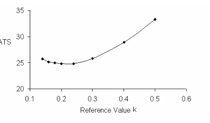
(45) Chapter 2 – Control Chart Definitions and Background Literature. Sparks (2000) investigated CCUSUM and Adaptive CUSUM (ACUSUM) schemes which were found to perform similarly. Three CUSUM components were recommended for detection of step shifts in the mean between 0.5σ and 4.0σ in size. Apparently heuristic design recommendations (with some theoretical basis) were used to choose the k values instead of optimisation. The ACUSUM method worked by adjusting the k value of a CUSUM scheme according to the optimum for the estimated step shift based on an EWMA forecast of the data. A regression model was used to find the required control limit coefficient for a given value of δ µ (via the relationship between optimal δ µ and the theoretical optimum value for k , k = δ µ /2, Sparks, 2000), the limits being adjusted at each serial observation. To prevent the monitoring tool becoming excessively powerful for small step shifts, a constraint was applied to the minimum value of k . CCUSUM was found to perform better than ACUSUM at large step shifts; however, ACUSUM is sensitive to the choice of λ in the EWMA forecasting equation.. Lack of optimisation and lack of a scalar. performance measure for a detection of a distribution of location shifts have resulted in an incomplete understanding of the performance of CCUSUM and ACUSUM methods from Sparks’ study.. Nevertheless, the thesis serves as an excellent. introduction to these tools demonstrating simple heuristic designs which are easy to implement.. Sparks (2003) demonstrated construction of CMA schemes and proposed a number of designs. The performance of CMA schemes in step and ramp location shift scenarios was compared to EWMA and CUSUM schemes. A comparison was yielded by measuring the relative loss efficiency (RLE) for step shifts and ramp shifts. It was found that the CMA design called “Plan 5” (design parameters are detailed in Appendix F) performed with small relative losses compared to a EWMA scheme with. λ equal to 0.15 at step shifts less than that for which the EWMA was optimised, i.e. <1 . However, the CMA scheme performed better on average over the entire 0.25 to 4 domain. The performance of CMA schemes compared to EWMA schemes on ramped location shifts was a different matter. An EWMA scheme with λ = 0.15 performed better than the CMA on all ramp location shifts from 0.005 /observation to 0.25 /observation. With this in mind, a CEWMA scheme may also perform well on ramped shifts if it is based on the EWMA statistic. A recommendation given in 28.

No results found