Zoom techniques for achieving scale invariant object tracking in real-time active vision systems

Rochester Institute of Technology

RIT Scholar Works

Theses Thesis/Dissertation Collections

9-27-2006

Zoom techniques for achieving scale invariant

object tracking in real-time active vision systems

Eric Nelson

Follow this and additional works at:http://scholarworks.rit.edu/theses

Recommended Citation

Zoom Techniques for Achieving Scale Invariant Object

Tracking in Real-time Active Vision Systems

by

Eric D. Nelson

A Thesis Submitted in Partial Fulfillment of the Requirements for the Degree of Master of Science in Computer Engineering

Supervised by

Associate Professor Dr. Juan C. Cockburn Department of Computer Engineering

Kate Gleason College of Engineering Rochester Institute of Technology

Rochester, New York July 2006

Approved By:

Dr. Juan C. Cockburn Associate Professor Primary Adviser Dr. Andreas Savakis

Professor and Department Head, Department of Computer Engineering Dr. Roy Czernikowski

Thesis Release Permission Form

Rochester Institute of Technology

Kate Gleason College of Engineering

Title: Zoom Techniques for Achieving Scale Invariant Object Tracking

in Real-time Active Vision Systems

I, Eric D. Nelson, hereby grant permission to the Wallace Memorial Library to repro-duce my thesis in whole or part.

Dedication

Acknowledgments

Abstract

In a surveillance system, a camera operator follows an object of interest by moving the camera, then gains additional information about the object by zooming. As the active vision field advances, the ability to automate such a system is nearing fruition. One hurdle limiting the use of object recognition algorithms in real-time systems is the quality of captured imagery; recognition algorithms often have strict scale and position requirements where if those parameters are not met, the performance rapidly degrades to failure. The ability of an automatic fixation system to capture quality video of an accelerating target is directly related to the response time of the mechanical pan, tilt, and zoom platform—however the price of such a platform rises with its performance. The goal of this work is to create a system that provides scale-invariant tracking using inexpensive off-the-shelf components.

Contents

Dedication. . . . iii

Acknowledgments . . . . iv

Abstract . . . . v

Glossary . . . . xi

1 Introduction. . . . 1

1.1 Active vision . . . 1

1.2 Thesis outline . . . 2

2 Background Theory and Related Work . . . . 4

2.1 An introduction to cameras . . . 4

2.1.1 Perspective projection . . . 6

2.1.2 Weak perspective projection . . . 7

2.1.3 Thin lens model . . . 9

2.1.4 Calibration . . . 10

2.2 Tracking . . . 11

2.2.1 Classification and clustering via color segmentation . . . 12

2.3 Focal length selection for optical zoom . . . 13

2.3.1 A steady-state Kalman filter . . . 13

2.3.2 Zoom invariant Kalman filter . . . 15

2.3.3 Controlling focal length . . . 23

2.4 Center of expansion . . . 26

2.5 Summary . . . 28

3 Dual Camera Zoom . . . . 30

3.1 Introduction . . . 30

3.2.1 Camera view correspondence . . . 31

3.2.2 Assisted control . . . 33

3.2.3 Control arbitration . . . 35

3.3 The experimental system . . . 36

3.3.1 Pan and tilt . . . 37

3.3.2 Zoom . . . 38

3.3.3 System organization . . . 43

3.4 Experiments on hardware . . . 43

3.4.1 Pendulum experiment . . . 43

3.4.2 Car experiment . . . 47

3.5 Summary . . . 50

4 Digital Scale Invariance . . . . 51

4.1 Choosing magnification for digital zoom . . . 51

4.2 Fixating with digital zoom . . . 53

4.3 Noise analysis . . . 53

4.3.1 Impact of image noise . . . 53

4.3.2 Simulations . . . 54

4.4 Display arbitration . . . 60

4.5 System Organization . . . 62

4.6 Experiments on hardware . . . 62

4.6.1 Pendulum experiment . . . 62

4.6.2 Car experiment . . . 67

4.7 Summary . . . 71

5 Conclusion . . . . 72

5.1 Summary of this work . . . 72

5.2 Future work . . . 72

5.2.1 Advanced tracking . . . 73

5.2.2 More cameras . . . 73

5.2.3 Advanced zooming camera . . . 73

A Miscellaneous . . . . 74

A.1 Derivation of constant velocity Kalman Filter . . . 74

List of Figures

2.1 Pinhole camera [12] . . . 4

2.2 Object size and object distance affect image size [12] . . . 5

2.3 Perspective Projection [12] . . . 6

2.4 Weak perspective projection [12] . . . 7

2.5 Lenses allow more light to enter the pinhole [12] . . . 8

2.6 Thin lens model . . . 9

2.7 Rotational calibration . . . 11

2.8 Image used to train color segmentation tracker . . . 12

2.9 Object motion used in figures 2.10-2.14 [30] . . . 17

2.10 Tracking with fixed focal length [30] . . . 18

2.11 Tracking with variable focal length [30] . . . 19

2.12 Tracking with variable focal length, withR∝f2 _{[30] . . . 20}

2.13 Tracking with variable focal length, withQ∝ 1 f2 [30] . . . 21

2.14 Tracking with variable focal length, withR∝f2 _andQ∝ 1 f2 [30] . . . 22

2.15 The effect of varying the “forgetting factor”γ [30] . . . 25

2.16 Example of center of expansion . . . 27

3.1 Camera correspondence . . . 32

3.2 Camera correspondence overhead view . . . 33

3.3 Sony EVI-D100 . . . 36

3.4 Step response for pan and tilt . . . 37

3.5 Block diagram for pan and tilt . . . 38

3.6 Zoom reading step response, lookup table, and magnification step response 39 3.7 Pseudocode to create magnification lookup table . . . 40

3.8 Zoom reading calibration . . . 41

3.9 Control arbitration block diagram . . . 42

3.10 Snapshots of pendulum experiment. . . 45

3.11 Pendulum results . . . 46

3.13 Car results . . . 49

4.1 Spinning coin problem . . . 52

4.2 Unfiltered digital zoom . . . 56

4.3 Kalman filter of digital zoom withRk = 10−4. . . 57

4.4 Kalman filter of digital zoom withRk = 10−8. . . 58

4.5 Kalman filter of digital zoom withRk = _h0R m2. . . 59

4.6 Digital zoom block diagram . . . 61

4.7 Scale invariance for panoramic camera . . . 63

4.8 Digital fixation for panoramic camera . . . 63

4.9 Scale invariance for zooming camera . . . 64

4.10 Digital fixation for zooming camera . . . 65

4.11 Display arbitration pendulum experiment . . . 66

4.12 Scale invariance for panoramic camera . . . 67

4.13 Digital fixation of panoramic camera . . . 68

4.14 Scale invariance of zooming camera . . . 68

4.15 Digital fixation of zooming camera . . . 69

List of Tables

Glossary

A

assisted control When a camera can only reliably fixate upon an object with both information acquired from its own sensors, along with information acquired from other cameras’ sensors. Needed when the target object falls out of the camera’s view. See autonomous control.

autonomous control When a camera can reliably fixate upon an object with informa-tion acquired only from its own sensors. Requires that the target object be in view of the camera. See assisted control.

C

calibration When various intrinsic and extrinsic properties of a lens are known, then the lens is considered calibrated. Angles and distances can be calculated with high accuracy in images acquired from a calibrated lens. In this work, calibration is limited to only knowing how many pixels in a captured image correspond to a degree on the camera’s pan or tilt axis. This partial calibration is low mainte-nance, but is obviously not as useful as full calibration where every parameter is known.

Cartesian Theater A metaphysical theater in the brain where reason and the senses, including vision, come together.

is generally fixed for optical zoom while it is flexible for digital zoom. See section 2.4.

control arbitration The process that decides whether to allow autonomous or assisted control for the zooming camera.

D

digital zoom When the size of an image is increased using upconversion and/or down-conversion. The target object’s detail does not increase. For large magnifica-tions, the resulting image can appear very pixelated. Compare to optical zoom, digital zoom is a fast operation and it has a very flexible center of expansion.

display arbitration The process that decides which camera shows the best view of the target object.

F

fixate The process of panning and tilting a camera so as to keep the target object in a camera’s view.

H

hybrid zoom A mixture of digital zoom and optical zoom. It takes advantage of the speed of digital zoom’s change of magnification and its center of expansion flexibility, with optical zoom’s increased detail.

K

M

magnification How much zoom happens; the ratio of the height of the image compared to the height of the object. Increasing the magnification makes the object appear to grow. Magnification is generally slow for optical zoom while it is nearly instantaneous for digital zoom.

N

notation • Arrays are shown in bold lowercase (e.g.a,b,c).

• Matrices are shown in capital teletype font (e.g.A,B,C).

• Subscript k+1|k indicates something calculated about time k + 1 given

information at timek.

• Images have an apostrophe,e.g.the image of pointP is shown asP0_{, and}

the height of an object,h, has an image of heighth0_.

• A line between two points, A and B, is represented as AB with length

AB.

• A dot represents derivative,e.g.positionxhas velocityx˙ and acceleration

¨ x. .

O

optical axis The line perpendicular to the image plane and passing through the pinhole of a camera.

expansion for optical zoom can change slightly as the lens properties change, the center of expansion is considered fixed when compared to digital zoom.

P

pan Rotating the camera horizontally, along the vertical axis, whereas all objects in the captured image appear to move either left or right.

S

stability Specifically in this work, the ability of the system to maintain fixation. A stable system can maintain fixation, while an unstable system cannot.

T

target object The object in the real world that the user wishes to capture in an image using the system.

tilt Rotating the camera vertically, generally along the horizontal axis orthogonal to the optical axis, whereas all objects in the captured image appear to move either left or right.

Chapter 1

Introduction

1.1 Active vision

In the early 1960s, researchers viewed computer vision as a relatively simple problem—if humans and multitudes of other organisms can so effortlessly see, then how difficult can it be to design a man-made system with similar attributes? The perception was that it would be mere decades before we were able to surpass the capabilities of a natural vision system— but nearly half a century later, research has indicated that human vision is considerably more complex than imagined.

A particular application of interest is the ability to recognize and interpret sign lan-guage, specifically American Sign Language (ASL). Used as the primary mode of commu-nication for millions worldwide, ASL is a language that communicates not only words but also the full gamut of human emotions, similarly to how inflexions in the spoken word can convey joy, sarcasm, or indifference. Therefore, to understand ASL as a human would, a computer must look at the hands, face, and body language of the signer.

The starting point of this daunting task is to interpret a single hand in real-time. Pre-ceding works present ways to track hands in real-time, such as Clark in [6], and to rec-ognize basic signs, such as Rupe in [22]. The missing bridge between the works is that the captured image must be conditioned appropriately for the recognition algorithm to be effective; object recognition algorithms often have strict scale and position requirements where if the requirements are not met, the performance rapidly degrades to failure. For example, the work of Yang et al.in [34] requires a60pixels×60pixels image while the work of Heisele et al. in [17] requires58 pixels×58 pixels. Other algorithms are more resistant to varying scale and position, but still have a preferred size, such as Rupe’s work which performs well between50pixels×50pixels and250pixels×250pixels, but works best with smaller images in that range.

The goal of this work is to develop a system that can reliably capture images of a

specific size and position determined by a higher-level process (e.g.an object

recogni-tion algorithm).

1.2 Thesis outline

Chapter 2discusses all relevant research done preceding this work, which includes a

zooming algorithm that aims to maximize focal length while guaranteeing that object fixa-tion will not be lost.

In the event of lost fixation—at least when there is no plan to reacquire fixation, such as in this work—an active vision system becomes unstable; observing a scene, or a specific object in a scene, is theraison d’ˆetre of the system, therefore if the object is out of view, the system can do nothing. Chapter 3proposes that by adding a second camera with fixed focal length, stability can be independent of the zoom action.

With stability no longer a concern, zoom only changes the size and resolution of the captured image. However, slow zoom response continues to prevent the ability to produce scale invariant images for all but slow-moving objects. In an effort to speed up zoom action without changing the hardware, Chapter 4uses digital zoom to remove mechanical time constants from zoom, which splits the zoom into two pieces: optical and digital. With digital zoom guaranteeing scale invariance, optical zoom only affects resolution.

Finally,Chapter 5concludes the work by listing contributions and recommending fu-ture work.

Chapter 2

Background Theory and Related Work

2.1 An introduction to cameras

In the 15th century, Brunelleschi published the first paper describing his understanding of image formation. The pinhole projection model was based on his experience with the original man-made imaging system, the pinhole camera, which is still widely used today among photographers. A pinhole camera is a favorite experiment of early optics courses, and can be easily constructed by poking a small hole in one side of an otherwise enclosed box, then replacing the opposite side of the box with a translucent material. As seen in Figure 2.1, light rays then pass through the pinhole to create an inverted image on the

Figure 2.2: Object size and object distance affect image size [12]

translucent side. Various scene and camera attributes determine the specific characteristics of that image, including the size, brightness, and orientation.

To demonstrate size, consider Figure 2.2 where object B is twice the height of both

A and C, yet the height of image B0 _{is identical to C}0 _{and twice that of A}0_{. The size of}

an object does not directly affect image creation, but rather it affects the angle of the light passing through the pinhole. Notice that objectC is half the distance from pinholeOasA

andB. Given that it is a geometry problem, the distance is important; the relative size of images depends not only upon size of an object, but also on its distance from the pinhole.

Figure 2.3: Perspective Projection [12]

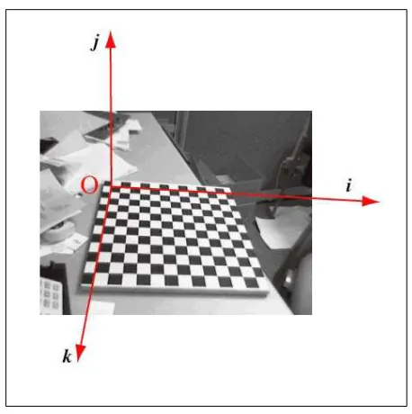
2.1.1 Perspective projection

All aspects of the pinhole model are used for the perspective projection, which for conve-nience is placed in coordinate system (O,i,j,k)—as seen in Figure 2.3—whereO is the pinhole;P is a point with imageP0_{; the image planeΠ}0 _{lies at distancef}0 _{fromO, and is}

orthogonal tok;C0_{is the image center where the optical axis intersectsΠ}0_.

PointP is mapped toP0 _by

x0 _=f0x

z (2.1)

y0 _=f0y

z (2.2)

m = f

0

z (2.3)

wheremis the magnification andz0 _=f0 _sinceP0 _{is onΠ}0_.

Figure 2.4: Weak perspective projection [12]

2.1.2 Weak perspective projection

Some approximations of the perspective projection have shown to be more practical. For example the weak perspective projection considers a group of points to all lie on the fronto-parallel plane, with depthz0as denoted in Figure 2.4 asΠ0. Effectively, perspective effects

within a single object are ignored such that pointP is mapped toP0 _by

x0 _{=−mx (2.4)}

y0 _{=−my (2.5)}

m =−f0

z0

(2.6) where physical constraints forcez0to be negative, making the magnificationmpositive.

(a) Pinhole camera

(b) With lens

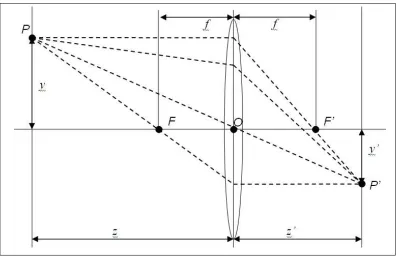
Figure 2.6: Thin lens model

2.1.3 Thin lens model

The projections presented above all assume an ideal pinhole camera, which allows only a single ray of light to reach the image plane. Real pinholes have finite size, such that smaller pinholes create faint images and larger pinholes create blurry images. As shown in Figure 2.5, lenses allow more light to pass through a small pinhole, producing a bright and sharp image.

A lens refracts, or bends, light such that it is redirected through a pinhole, or focal point

F. The lens’s shape, thickness, and material determines the nature of refraction. With the thin lens model in Figure 2.6, which assumes the thickness of the lens is infinitesimally small,z0 _{is not necessarily equivalent tof}0 _{but rather}

1 f =

1 z0 −

1

wheref =f0 _{is the focal length. The magnification is defined as}

m= z0 z =

h0

h (2.8)

where his the height of an object and h0 _{is the height of its image. For a zoom lens, the}

focal length varies, allowing the magnification to change.

A real zoom lens is generally made up of dozens of individual moving lenses. Depend-ing on the quality of the lens and the application for which the lens is used, the thin lens model can still be applied [30, 33].

For more information about projections and lenses, see [12, 27].

2.1.4 Calibration

To measure an image it is necessary not only to understand the projection, but also to know specific attributes of the camera and lens. Some intrinsic parameters include focal length, skew, principal point, distortion. Extrinsic parameters include rotation and translation.

The acquisition of these attributes is called calibration [24, 12]. Depending on the complexity of the system as well as the attributes necessary, calibration can be costly. When zooming, different methods of tracking are used, as shown in [15, 11, 28, 29, 16, 30], all of which require calibration of the zoom lens, a process more costly than constant focal length camera calibration [21].

For some applications, it is possible to consider the effect of certain parameters as negligible. Such assumptions increase the measurement error, but a closed-loop control system can reduce that error. When fixating it is essential to approximate a pixel to camera angle near the center of the image. To acquire this parameter, measurements need to be conducted as shown in Figure 2.7. Rotational calibration can be donea prioriand therefore does not affect real-time performance.

Figure 2.7: Rotational calibration

If a camera provides real-time odometry, then performance is unaffected. Since off-the-shelf cameras with zoom odometry are available, it is possible to completely model the camera in a manner that is favorable to real-time systems [30].

2.2 Tracking

Figure 2.8: Image used to train color segmentation tracker

2.2.1 Classification and clustering via color segmentation

This algorithm denotes a range of colors as being part of the target object, or foreground, while every other color is part of the background. Different color spaces of interest are RGB, rgb, and YUV. In this work, the nonlinear color space hue-saturation-value (HSV) is used, sometimes referred to as hue-saturation-intensity (HSI) or hue-saturation-lightness (HSL). Frame grabbers commonly acquire images in the linear RGB space, so an example of a conversion to HSV from [18] is

V = max(R, G, B)

S =

 



(V −min(R, G, B))∗255/V, ifV 6= 0 0, o.w.

H =

    

   

(G−B)∗60/S, ifV =R 180 + (B−R)∗60/S, ifV =G 240 + (R−G)∗60/S, ifV =B

After initial segmentation, the morphological operations of dilation and erosion im-prove the contiguousness of the foreground—known as clustering. A connected compo-nents algorithm then labels each of the separate foreground regions, with the largest of those regions denoted as the target object.

Figure 2.8 shows the image used to train the color segmentation tracker for red objects. As a sidenote, future chapters use this tracker to test ideas presented in this work. While this tracking algorithm is rather simplistic, it does provide a robust and easy-to-maintain algorithm, that is proven in real-time systems; it serves as a proof-of-concept.

2.3 Focal length selection for optical zoom

Tracking information is essential in determining the optimal focal length that maximizes resolution while maintaining fixation because focal length—or more appropriately zoom— acts as a measurement gain, amplifying both resolution and tracking error. Multiple sources present ways to accomplish that, including Tordoff in [30] and Denzleret al.in [10].

Sznaieret al.propose a different method altogether by using robust control to make an active vision system resistant to changes in focal length. Their method is limited in that wider ranges of focal length degrade performance [26, 25].

The Tordoff method, because it is proven in a real-time environment, is presented below.

2.3.1 A steady-state Kalman filter

From a practical point of view, a Kalman filter is a recursive algorithm that makes estimates and predictions about the state of a system based upon noisy data from multiple sources, such as from a model and measurements. The Kalman filter combines, in an optimal fash-ion, the data points to estimate the current state and predict future states [1, 20].

based upon its angle relative to the optical axis, with state vectorp =

³

φ,φ˙

´_>

whereφis the pan (or tilt) angle of the camera needed to fixate directly upon the target object. For simplicity, the equations only account for a single dimension (i.e.pan), but adding extra orthogonal dimensions (e.g.tilt) is trivial. The linear model is:

p_k+1 =Fkpk+uk+qk (2.9)

where subscriptkdenotes the discrete frame;uk = (−θk,0)>is the control input whereθk

is the change in camera angle between time k−1andk; andqis the process noise drawn from a zero mean Gaussian noise sequence with covarianceE£q_kq>

k

¤

=Qk. For constant

velocity motion, the state transition matrixFkis,

Fk =F=



 1 ∆T

0 1



 _(2.10)

where ∆T is the sampling time, such that ∆T = tk − tk−1 To complement the model,

measurements of an image projected as a 3D to 2D mapping such that

mk=Hkpk+rk (2.11)

wheremis the measurement;rkis the measurement noise drawn from a zero mean

Gaus-sian noise sequence with covarianceE£rkr>k

¤

=Rk; andHkis given by

Hk=H=

³

1 0

´

(2.12) where H1 = 1 exhibits fixed focal length of unity—dynamic focal length would create a

time-varying filter. The measurement is then anx-coordinate in a unit width image (−1 2 <

x < 1 2.

There are three stages in the Kalman filter: prediction, measurement, and correction.

indicates an estimation of the state at timek+ 1given all the information available at time

k.

ˆ

p_k+1|k = Fkpˆk|k+uk (2.13)

ˆ

Pk+1|k = FkPˆk|kF>k +Qk (2.14)

ˆ

mk+1|k = Hk+1pˆk+1|k (2.15)

ˆ

Mk+1 = Hk+1Pˆk+1|kH>k+1+Rk+1 (2.16)

In themeasurementstage, the expected measurement is compared to the actual mea-surement, giving the innovationνk+1 defined as

νk+1 = mk+1−mˆk+1|k (2.17)

Thecorrectionstage then recalculates the state based ona posterioriknowledge of the

measurement as follows:

Wk+1 = ˆPk+1|kH>k+1Mˆ

−1

k+1 (2.18)

ˆ

p_k+1|k+1 = ˆp_k+1|k+Wk+1νk+1 (2.19)

ˆ

Pk+1|k+1 = ˆPk+1|k−Wk+1Mˆk+1W>k+1 (2.20)

Initial values forpˆ₀, Pˆ0,Q, andRmust be provided. The derivation of the filter update

equations is available in the work of Bar-Shalomet al.[3].

2.3.2 Zoom invariant Kalman filter

Adding zoom to the filter does not change the model in Equation 2.9, but it does affect the measurement in Equation 2.11, such that

Hk =

³

fk 0

´

(2.21) wherefkis the camera’s focal length at timek. With non-constantH, the filter becomes a

To simplify the time-varying filter, Tordoff presented a method to make the filter behave identically to the steady-state filter by either scaling measurement noise with focal length

Rk = fk2R (2.22)

or scaling process noise with the inverse of focal length,αk = 1/fk

Qk = α2kQ (2.23)

By using either equation 2.22 or 2.23, the filter is unaffected by changing focal length, but using both equations actually improves fixation error—as shown by simulation.

Simulations

For proper comparisons, each of the following trials—originally presented in [30]—undergo the same motion: an object begins at position φ = −60◦ _{with velocity φ}˙ _{= 30}◦_s−1_{, and}

continues until φ = 30◦ _{whereupon constant acceleration is applied until φ}˙ _{= −30}◦_s−1_;

the object then continues until φ = −60◦_{—Figure 2.9(a) and Figure 2.9(b) illustrate that}

motion. Figure 2.9(c) shows the focal length for trials involving variable zoom.

The initial conditions for the trials arep= (m1, m1−m0)>,f = 1,r =.02

(approxi-mately 3.2 pixels in a160×120image), andQas derived in Appendix A.1 is

Q= 10−6×



 ∆T

3

3

∆T2

2 ∆T2

2 ∆T



 _(2.24)

where∆T = 1

30s. The pan/tilt platform is assumed ideal in thatθverg,k+1 = ˆφk+1|k. Noise

is added to the measurements with standard deviation of0.02.

The trial with fixed focal length, Figure 2.10, serves as a baseline; a zoom-invariant filter should match this response.

(a) (b)

(c)

(a) (b)

(c)

(a) (b)

(c)

(a) (b)

(c)

(a) (b)

(c)

Figure 2.13: Tracking with variable focal length, withQ∝ 1

(a) (b)

(c)

Figure 2.14: Tracking with variable focal length, withR∝f2 _andQ∝ 1

By scaling measurement noise with focal length, Figure 2.12 shows prediction identical to the baseline—a zoom-invariant filter. The fixation error is still affected by zoom level. Figure 2.13 presents another zoom-invariant filter while scaling process noise with the inverse of focal length.

Figure 2.14 shows that estimation actually improves when using both Equation 2.22 and 2.23. This filter is the best fitted for changing focal length; performance of the filter is not zoom invariant but rather it isimprovedby the presence of zoom.

For more details about the simulations, see [30].

2.3.3 Controlling focal length

The preceding simulations used predetermined focal length, proving that changing focal length affects fixation error. This section looks to maximize zoom while keeping fixation error bounded; the amount of fixation error is unimportant as long as the target object remains in the image.

A critical piece of zoom control is the innovation calculated from the Kalman filter, which represents the error between what is expected in the constant velocity model and what is observed. This error encapsulates target object acceleration, and other noise present in the system. The desired focal length is inversely proportional to the variance of the innovation.

From [30]:

In the context of Kalman filtering, [bounded error] can be interpreted as specifying a confidence bound on the innovation

p(|ν|< ψ)≥ζ (2.25) whereψ is the boundary location, andζthe confidence that is required. If the innovation is 1D, as in the previous simulations, then for a matched filter ν

confidence interval) then the ideal variance is var[ν] ≈ ψ2_{/24. Since ν scales}

with focal length, we wish to zoom out if the variance ofνis too high, and the control law becomes

f2

k+1 ≤

ψ2

var[νk]

(2.26) The case of a 2D innovation is similar, as ν again scales with zoom. For a matched filter ν is sampled from a 2D Gaussian, which will generally not be independent in the image axes. . . The requirement is then that the maximal variation in any direction is within the bound ψ. For the “one in a million” bound, the control law is

f2

k+1 =

ψ2

24kcovar[νk]k₂

(2.27) where the 2-norm of the covariance gives the maximum variation (i.e. the largest eigenvalue of the covariance matrix). To enforce [maximum resolu-tion,] the inequality is replaced by equality, and zoom is controlled to always make the covariance touch this boundary.

He continues:

In order to fulfil the bounding conditions, an estimate of the innovation (co–)variance is required. For changing target dynamics, this variance will change over time, and so the statistics of the most recent errors are required. A simple approach is to maintain an exponentially weighted sequential estimate of the covariance

covar[¯νk]≈γ

¡

νkν>k

¢

+ (1−γ)covar(¯νk−1) (2.28)

whereγis the “forgetting factor” in the range0< γ <1, and varyingγas1/k

(a) γ= 0.02 (b) γ= 0.10

(c)γ= 0.50

In practice, there are some subtleties to such a scheme when zoom is chang-ing. First asνkis scaled byf, the variance calculation must take into account

changes of zoom. The zoom-normalized variance is therefore calculated: covar[¯νk]≈γ

¡

νkν>k

¢

f2

k

+ (1−γ)covar[¯νk−1] (2.29)

Practically, these equations cause the camera to zoom–in when the velocity is constant and zoom–out whenever there is any acceleration. A largerγallows for quick adjustments in zoom level, while a smallγ allows for slower adjustments, see Figure 2.15.

Zooming in can cause instability as it increases the possibility of the target object leav-ing the image, while zoomleav-ing out only costs detail. Calculatleav-ing two covariances, one with a largeγ and another with a smallγ, then using the value with the small focal length cre-ates a conservative zoom–in and a faster zoom–out. This method is safe with respect to bounding the fixation error, but at the expense of resolution.

2.4 Center of expansion

The focal length determines how much zoom, but it does not determine where to zoom. Optical zoom lenses generally zoom around the center of the image, called the center of expansion, defined by Willson in [33]:

Given two images taken at different magnifications, exactly one position in the scene in both images will remain in the same place on the image plane. This position is called the “center of expansion” between the two images. More precisely, given two imagesI1 andI2taken at two magnificationsm1 andm2,

and givennreference pointsP1. . . Pnin imageI1and the corresponding points

Q1. . . Qnin imageI2, the center of expansionC satisfies the constraint

(C−Pi) = k(C−Qi) ∀ i= 1. . . n (2.30)

where

(a) Zoomed out view

(b) Zoomed with top–center center of expansion (c) Zoomed with bottom–left center of expansion

Willson describes center of expansion in the context of calibrating zoom lenses, but it applies for both optical and digital zoom. Figure 2.16 shows an example of 2.8X zoom magnification with different centers of expansion. The magnification determines the size of the image, while the center of expansion determines what is shown in the image.

For optical zooming, the center of expansion is usually the same as—or very close to— the principal point of the lens, which is the intersection of the optical axis with the image plane. The center of expansion can change slightly as other lens parameters change, but can generally be considered fixed. A fixed center of expansion is difficult when trying to zoom on a specific object; if that object is not on the principal point, then the object will eventually fall off the edge of the image when zooming in. The only way to move the center of expansion onto the target object is to either a) move the target object or b) move the image axis and image plane,e.g.pan and/or tilt the camera. Assuming that the former is not possible, the only choice is to move the camera. Therefore, the goal of scale invariance is not only limited by zoom response but also pan and tilt response.

With digital zoom or advanced zoom lenses [32], the center of expansion is more flexi-ble as it can be instantaneously placed anywhere on the image plane.

2.5 Summary

For image perception, it is important to understand how images are captured. While not well-suited for real-time applications, the perspective projection is an accurate model of a camera. The less precise weak perspective projection ignores most perspective effects, making it less computationally intensive and therefore appropriate for real-time applica-tions. Combined with a lens model and a tracking algorithm, projections describe the sensing aspect of active vision.

resolution. This compromise was addressed by maximizing resolution while bounding fixation error.

Chapter 3

Dual Camera Zoom

3.1 Introduction

The presence of zoom can improve the perceptibility of an acquired image by either mag-nifying detail or broadening the field of view. However, since higher focal lengths confine the periphery, both improvements cannot occur simultaneously.

Tordoff elaborates in [30] saying “consider a camera operator viewing a stationary ob-ject (it might be a golf ball on the fairway, or a gnu on the veld). While stationary, the operator’s instinct is to zoom in. However, as soon as the object starts to move, the camera-man will react both by attempting to track and by zooming out. As tracking is restored, say at constant angular velocity, the operator may have sufficient confidence to zoom in again, but if subsequently the tracked object moves unexpectedly he will surely once more zoom out. It appears that the camera operator is reducing tracking error to an acceptable distance in the image, where ‘acceptable’ means better than half the image dimension—at worst he wishes to retain sight of the object on the image plane.”

Now consider that the camera operator does indeed lose sight of the object. Recog-nizing that, he pulls his eye away from the camera, finds the object, and then adjusts the camera accordingly. In this case, the naked eye serves as a fixed focal length, panoramic camera.

Similar methods are presented in the works of Greiffenhangenet al.in [13] and Huang

et al.in [19]. They differ from this work in that their panoramic camera serves as a station-ary overseer—it is mounted on the ceiling. In this work, both cameras rotate from nearly the same viewpoint.

This chapter explains how to detect when fixation is lost, then subsequently how to recover. A real-time system which implements the algorithm is presented along with ex-periments that validate the method.

3.2 Recovering fixation

3.2.1 Camera view correspondence

Communication between two rotating cameras requirescamera view correspondence. Con-sider Figure 3.1 whereZandP, included as either labels or subscripts, represent the zoom-ing and panoramic cameras;kis on the optical axis of cameraZat an arbitrary but constant time t0; image centers CZ0 and CP0 are situated such that line CZ0 CP0 is parallel toi with

length d; image planesΠ0

Z andΠ0P are both orthogonal to k at timet0. The center of the

target object,T, is related to the image centers such that

¡ C0 PT ¢ i = ¡ C0 ZT ¢

i+d (3.1)

¡ C0 PT ¢ j = ¡ C0 ZT ¢ j (3.2) ¡ C0 PT ¢ k = ¡ C0 ZT ¢ k (3.3)

where subscripts k andi indicate the components of the line along the appropriate axis,

e.g.the pythagorean theorem reads as

C0

PT =

Figure 3.1: Camera correspondence The angle of lineC0

ZT on the plane with basis ofiandjis represented by pan angleθZ.

Similarly, the angle of lineC0

PT on the same plane isθP. The same lines have tilt angles

φZandφP on the plane with basis ofiandk.

SinceC0

Z andCP0 differ only by a translation in theidirection, then the tilt angles are

identical

φZ =φP (3.5)

leading to the simplified view shown in Figure 3.2 where

x = ¡C0

ZT ¢ i = ¡ C0 PT ¢

i−d (3.6) z0 =

¡ C0 ZT ¢ k= ¡ C0 PT ¢ k (3.7)

wherez0is the distance to the fronto-parallel plane. The pan angles are related by

θZ(θP, d, z0) = tan−1

"µ

cot (θP)−

d¶−1#

Figure 3.2: Camera correspondence overhead view

3.2.2 Assisted control

When fixating with a single camera, the desired camera angles—θandφ—placeT0 _atC0_.

When T0 _{is onΠ}0_{, then a tracker can be used to calculate the angles, called autonomous}

control. However if T0 _{is off the edge of Π}0_{, then assisted control is necessary, which}

requires a second camera.

Consider framek whereT0 _{is on Π}0 _{for both cameras, thenz}

0,k is the distance of the

image planes to the fronto-parallel plane

z0,k =

d

cot (θP,k)−cot (θZ,k)

(3.9) Now say for some future frame n > k that T0

Z is off image plane Π0Z, butTP0 remains on

ΠP. Then θP andφP can be computed using assisted control. Equation 3.5 givesφZ, and

θzcan be found using Equation 3.8 ifznis known. Using the basic lens equation, originally

presented as Equation 2.8,

z0

z = h0

wherehis the height of the object, then for framenandk zn =

hn

h0

n

z0

n (3.11)

zk =

hk

h0

k

z0_k (3.12) By assuming image distancez0_{and object heighthdo not change over time,i.e.}

z0_k = z_n0 (3.13)

hk = hn (3.14)

then zn zk = h 0 k h0 n (3.15)

zn = zkh

0

k

h0

n

(3.16) In addition, to account for object rotations about the optical axis, one may also consider measured widthw0_{, combining it with height to give measured areaA}0 _=h0_w0_{. Now}

zn=zk

s A0 k A0 n (3.17) which with Equation 3.8 gives the desired pan angle.

Sources of error

The performance of assisted control depends upon precision of the angle, position, and height measurements. Without accurate calibration of the cameras, camera odometry may be used for measurements of θ and φ. For that case, it is recommended that frame k

correspond to when the pointsT0

ZandTP0 are as close to their respective image centersCZ0

andC0

P as possible, to minimize the effect of inaccurate calibration.

3.2.3 Control arbitration

Like most vision tasks, switching between assisted control and autonomous control is an action naturally suited to humans, as the Cartesian Theater holds assumptions about the scene [9]. However, given the state of modern computer perception, particularly real-time perception, a single-camera has no notion of how an object shouldlook; deciphering be-tween target deformities, rotations, and fixation losses is not obvious.

In a dual-camera system, a comparison can be made between the cameras’ images—if measurements do not make sense, then fixation must be lost. An assumption that cameraP

always has the object in view is made for simplicity; cameraP is more stable, so if it loses fixation then the system is unstable.

The target object is considered in view of the zooming camera when the following conditions hold true

h0

P −∆≤h0Z

fP

fZ ≤h0

P + ∆ (3.18)

w0

P −∆≤wZ0

fP

fZ ≤w0

P + ∆ (3.19)

where ∆ is the uncertainty of the tracker’s results; w0 _{is the measured width; h}0 _{is the}

measured length; f is the focal length; and subscriptsZ andP represent the zooming and panoramic cameras, respectively. If both of these hold true, then thecontrol arbitratormay decide to allow cameraZ to resume autonomous control.

The transition from autonomous control to assisted control is seamless, but the arbitra-tor must not resume autonomous control too soon as the zooming camera’s filter will have gonen−kframes without receiving a measurement. A safety delay,tsafety, to allow camera

Z’s filter to receive measurements is recommended such that

Figure 3.3: Sony EVI-D100

wheretassisted ≡ n−kis how long assisted control was used,αis a weight appropriate for

the filter, andtmaxis the maximum possible amount of safety time needed to regain stability

in the event of lengthy object loss.

3.3 The experimental system

To test the effectiveness of assisted control, a system was constructed using a pair of Sony EVI-D100 cameras, shown in Figure 3.3.

0 0.2 0.4 0.6 0.8 1 1.2 1.4 1.6 −100 −80 −60 −40 −20 0 20 40 60 80 100 Time (s) Angle (degrees)

Pan Step Response

(a) Pan

0 0.2 0.4 0.6 0.8 1 1.2 1.4 1.6 −20 −15 −10 −5 0 5 10 15 20 Time (s) Angle (degrees)

Tilt Step Response

(b) Tilt

Figure 3.4: Step response for pan and tilt

Communication from the cameras to the controller utilized the Sony VISCA protocol over RS-232 lines, connected to a PC powered by two Pentium Xeon 2.8 GHz with Hy-perthreading CPUs. Two Osprey 100/200 were used as a frame grabber, which have the capability of capturing images at 30 fps at 320 x 240 non-interlaced or 640 x 480 interlaced.

3.3.1 Pan and tilt

Figure 3.5 shows the step response for pan and tilt. Pan and tilt have similar plants, which differ on by velocity limits: 300◦_{/s for pan and 100}◦_{/s for tilt. Through experimentation,}

the transfer function was found to be approximately

T(s) = ¡ 1

1 + s

15

¢₂ (3.21) which includes neither the velocity limit or the 100ms delay between control signal and response.

Figure 3.5: Block diagram for pan and tilt

both object motion and camera angle. Calibration parameters convert the image measure-ments back to physical angles.

3.3.2 Zoom

Since the EVI-D100 features focal length odometry, a zoom lens model is unnecessary. However, the odometry is not ready out-of-the-box as a number between 0 and 16384

inclusive—referred to as the raw reading—represents focal length. The step response of the raw reading is shown in Figure 3.6(a), showing a 150 ms delay to initial response and a settling time of1.5s. The response is velocity-limited to7000 units_s .

0 0.2 0.4 0.6 0.8 1 1.2 1.4 1.6 1.8 0 2000 4000 6000 8000 10000 12000 14000 16000 Time (s) Camera reading

Zoom Step Response

(a) Raw

0 2000 4000 6000 8000 10000 12000 14000 16000 18000 1 2 3 4 5 6 7 8 9 10 11 Camera Reading Magnification

Zoom Lookup Table

(b) Lookup table

0 0.2 0.4 0.6 0.8 1 1.2 1.4 1.6 1.8 1 2 3 4 5 6 7 8 9 10 Time (s) Magnification

Zoom Step Response

(c) Magnification

1. forn = 0toN

2. reading⇒(max reading−min reading)∗ n N

3. Zoom toreading

4. Wait for zoom to complete

5. size[n]⇒average size of target inmimages 6. magnification[n]⇒size[n] /size[0]

7. end for

Figure 3.7: Pseudocode to create magnification lookup table

(a) Magnification=1X (b) 3X

(c) 7X

Figure

3.9:

Control

arbitration

block

3.3.3 System organization

The control of each camera is almost entirely independent, as shown in Figure 3.9, allowing for parallelism to help real-time performance; control arbitration is the only step needing synchronization.

3.4 Experiments on hardware

3.4.1 Pendulum experiment

In the interest of comparison via repeatability, the first experiment is a horizontally swing-ing pendulum with a red ball as its bob. The parameters used in the test include

∆ = 3pixels

r = 0.01(3 pixels / 320 pixels)

R = r2 = 10−4

γ = 0.1

d = 13cm

∆T = 33ms

tmax = 1s

α = 1

Q = 10−6



 ∆T

3

3 ∆T

2

2 ∆T2

2 ∆T





See Appendix A.1 for derivation ofQ.

Figure 3.10 shows how the target object is lost and recovered using snapshots from the dual-camera trial. In frame 30, the ball is stationary, indicated by the large magnification of the zooming camera. By frame 43, the ball has been released, showing that the zooming camera quickly lost the ball. In frame 215 the ball has been recovered but leaves the view by frame 231, then again re-enters in frame 235 before being fully in view by frame 239.

All results of the pendulum experiment are contained in Figure 3.11. The zooming cam-era’s fixation is illustrated in Figure 3.11(a), where the expected image height is denoted by the dotted black line, and the measured image height by the solid area. When the expected and measured height do not match, fixation is lost. The camera arbitrator, Figure 3.11(d), enabled the pan angle of the zooming camera to follow the bob, Figure 3.11(c).

Because of the less aggressive zoom, the single camera trial keeps the object in view throughout Figure 3.11(b). The average zoom of the dual-camera method is 1.5X better despite frequently resorting to the panoramic view, as shown in Figure 3.11(e) and Fig-ure 3.11(f). The zoom improvementI is calculated as

I = fdual fsingle

(3.22) where fdual and fsingle are the focal lengths for the dual- and single-camera methods,

030 030

043 043

215 215

231 231

235 235

239 239

Panoramic Camera Zooming Camera

5 10 15 20 25 0 20 40 60 80 100 120 140 160 180 200 Time (s) Width (pixels)

Measured Width (Pendulum)

Zooming camera (actual) Panoramic camera Zooming camera (expected)

(a) Fixation of dual-camera method

5 10 15 20 25 30 35

0 20 40 60 80 100 120 140 160 180 200 Time (s) Width (pixels)

Measured Width (Pendulum)

Zooming camera (actual) Panoramic camera Zooming camera (expected)

(b) Fixation of single-camera method

5 10 15 20 25

−40 −30 −20 −10 0 10 20 30 40 Time (s)

Pan Angle (degrees)

Pan Angles of Panoramic and Zooming Cameras (Pendulum)

Panoramic camera Zooming camera

(c) Dual-camera pan angles

5 10 15 20 25

0 1

Time (s)

0=assisted, 1=autonomous

Control Arbitrator (Pendulum)

(d) Decisions of control arbitrator

5 10 15 20 25

1 2 3 4 5 6 7 Time (s) Magnification

Zoom Level Comparison (Pendulum)

Single camera Dual camera

(e) Side-by-side zoom level comparison

5 10 15 20 25

0.5 1 1.5 2 2.5 3 3.5 Time (s) Improvement (Magnification/Magnification)

Zoom Level Improvement (Pendulum)

3.4.2 Car experiment

Of course, the primary objective of dual-camera zoom is not to increase zoom level, but rather to increase stability in the presence of zoom. A second experiment was run to fur-ther exhibit this trait. One drawback of the pendulum experiment is that if the zooming camera loses fixation, the nature of pendulum motion allows the camera to regain fixation periodically; see Figure 3.11(b) for time 1–3 s.

A radio-controlled car provides sporadic movements that demonstrate the advantages of having a second camera. In fact, the experiment could not be run on the single-camera method without nearly eliminating zoom. This car experiment uses parameters identical to the pendulum experiment, except with ∆ = 5pixels to account for the irregular shape of the car, andψ = 4.0to keep the zoom aggressive.

Frames 85, 415, and 800 of Figure 3.12 show large magnification in the zooming cam-era, while frame 260 shows similar zoom levels between the two cameras. Frames 225 and 700 show complete losses of fixation in the zooming camera, which correspond to the fast horizontal movements shown in Figure 3.13(a). Fixation loss is especially evident att= 8

085 085

225 225

260 260

415 415

700 700

800 800

Panoramic Camera Zooming Camera

5 10 15 20 25 −60 −40 −20 0 20 40 60 Time (s)

Pan Angle (degrees)

Pan Angles of Panoramic and Zooming Cameras (Car)

Panoramic camera Zooming camera

(a) Dual-camera pan angles

5 10 15 20 25

0 1

Time (s)

0=assisted, 1=autonomous

Control Arbitrator (Car)

(b) Decisions of control arbitrator

5 10 15 20 25

0 50 100 150 200 250 300 Time (s) Width (pixels)

Measured Width (Car)

Zooming camera (actual) Panoramic camera Zooming camera (expected)

(c) Fixation of dual-camera method

5 10 15 20 25

1 2 3 4 5 6 7 Time (s) Magnification

Magnification of Zooming Camera (Car)

(d) Zooming camera zoom level method

3.5 Summary

The goal of this chapter was not to simply improve stability in the presence of zoom, but rather to make stability independent of zoom. A human camera operator’s method of object recovery was used as motivation.

The fixation system needed information about how the target object should look before a determination of quality fixation could be asserted. This information was collected using a second camera. An understanding of the geometry comprising camera view correspon-dencewas integral in understanding key concepts such asassisted control, which is when one camera is controlled using another camera’s sensors. If a camera loses fixation it must switch to assisted control to prevent system instability. When a camera has enough infor-mation to control itself, the termautonomous controlis appropriate. Thecontrol arbitrator

decides which type of control is appropriate.

Chapter 4

Digital Scale Invariance

The long time constants of zoom lenses has proven to be a hindrance not only to stability, but also to scale invariant tracking. A zoom lens must follow object motion to maintain image size, so a slow-moving lens is limited to all but slow-moving objects. An alternative way to change scale is through digital zoom—a concept integral to digital imaging—which magnifies via interpolation and decimation.

While digital zoom is fast, optical zoom’s most valuable characteristic is its ability to adjust image detail and context. The goal of this chapter is to create a hybrid zooming technique which combines the strengths of digital and optical zoom to mask their individual weaknesses.

4.1 Choosing magnification for digital zoom

The exact magnification that provides scale invariance may be obtained in real-time now that zoom changes instantaneously. To preserve image size, it is necessary that the magni-ficationf is proportional to the object distancez0. Using the measured area to approximate

z0 can handle translations in any direction, but cannot handle rotations well. This method

(a) Spinning coin. http://www.startcreative.co.uk/images/Coin rotate.jpg

(b) Adjusting focal length with image area [31]

An alternative solution to prevent unwanted zoom oscillations is to consider the mea-sured length and width separately. If height alone is used to calculatez0, then zoom

oscil-lations do not appear; the width is what oscillates. Of course, this is not a general solution because a different situation could present height as the problem instead of the width.

Therefore, to consider both height and width, the magnification m to produce scale invariance is

mk =

h0

0

max (h0

k, w0k)

(4.1) whereh0

0is the desired image dimension,h0kis the image height, andw0kis the image width.

All values are for frame at timek. This method creates a bounding square around the object which is resistant to the spinning coin.

4.2 Fixating with digital zoom

Digital images not only allow for rapid zoom, but also for movable image center which can be adjusted to match the tracker’s position measurement. Therefore, fixation error can be eliminated. The reduction of fixation error has been studied in earlier chapters, as well as in many works such as [8, 7].

4.3 Noise analysis

4.3.1 Impact of image noise

Image measurements inherently have noise. When measuring the height of an image,

h0

m,k =h0k+rk (4.2)

whereh0

m,k is the measured height,h0kis the actual height, andris image noise drawn from

a zero mean Gaussian noise sequence with covarianceE£rkr>k

¤

A large signal-to-noise ratio (SNR), i.e.h0

k À rk, can make noise effects negligible,

where

SNR= h

0

k rk

(4.3) However since the SNR varies with measured height, large magnifications are more sus-ceptible to noise. The effect of image noise varies with resolution, which manifests itself as shaky zoom. To decrease this shakiness, magnification can be calculated such that

m = h

0 0 ˆ h0 k (4.4) where ˆh0

k is the estimated image height. When SNR is large, the measurement can be

assumed more accurate than when SNR is small—consequently when measurements are noisy, a model is appropriate.

The height measurement depends not only on noise, but also upon the state of the system such that

h0

k =

fkhk

zk

(4.5) which was derived from Equations 2.8 and 2.7 where fk is the camera focal length,zk is

the distance to the target object, andz0

k =fkbecausezkÀzk0.

A filter which does not account for dynamic SNR may only be effective under certain conditions. A Kalman filter as presented in Section 2.3 will is used.

4.3.2 Simulations

To make clear the need for a proper filter, experiments are run using various filters—each of which is fed identical object motion and measurement noise. An object of height 0.35m begins at z = 0.5 m with velocity z˙ = 0.5 m/s away from the camera. Upon reaching

Filter Error (approx 2-norm)

None 318.2

High image noise covariance 1223.2 Low image noise covariance 186.1 Variable image noise covariance 111.7 Table 4.1: Filter comparison in presence of image noise

Figure 4.2(c). The focal length throughout simulation isf = 35mm. When applicable,

Q= 10−6_×



 ∆T

3

3 ∆T

2

2 ∆T2

2 ∆T





The unfiltered run is shown in Figure 4.2(a). Notice that the noise escalates for largez. Figure 4.3 shows a Kalman filter with R = 10−4_{. This filter relies substantially on}

the model, which makes it resistant to the high-noise measurements: a desirable behavior. However, when noise is low, an unwanted delay appears between actual state and estima-tion.

Figure 4.4 on the other hand has a smallerR= 10−8_{. It does not rely heavily upon the}

model for the simulated distances, which leads to less resistance to noise.

A filter which adapts itself to changing conditions is shown in Figure 4.5, whereRk =

R

h0

m2 andR = 10

−8_{. The result is a filter that is resistant to high noise without adversely}

affecting the response when noise is low.

0 2 4 6 8 10 12 14 16 18 −1 0 1 2 3 4 5 Time (s) Distance (m) Estimation Measured Estimate Actual (a) Estimation

0 2 4 6 8 10 12 14 16 18

0 5 10 15 20 25 30 35 40 45 50

error 2 norm: 318.2362

Time (s)

% error

% error

(b) Percent error

0 20 40 60 80 100 120

−1 0 1 2 3 4 5 Pixels Distance (m)

Distance vs Pixels

(c) Distance vs Pixels

0 2 4 6 8 10 12 14 16 18 −1 0 1 2 3 4 5 Time (s) Distance (m) Estimation Measured Estimate Actual (a) Estimation

0 2 4 6 8 10 12 14 16 18

0 5 10 15 20 25 30 35 40 45 50

error 2 norm: 1223.1724

Time (s)

% error

% error

(b) Percent error

0 0.5 1 1.5 2 2.5 3 3.5 4

−1 0 1 2 3 4 5 Time (s) Distance (m) Pulse Response Measured Estimate Actual

(c) Pulse response

0 2 4 6 8 10 12 14 16 18 −1 0 1 2 3 4 5 Time (s) Distance (m) Estimation Measured Estimate Actual (a) Estimation

0 2 4 6 8 10 12 14 16 18

0 5 10 15 20 25 30 35 40 45 50

error 2 norm: 186.0805

Time (s)

% error

% error

(b) Percent error

0 0.5 1 1.5 2 2.5 3 3.5 4

−1 0 1 2 3 4 5 Time (s) Distance (m) Pulse Response Measured Estimate Actual

(c) Pulse response

0 2 4 6 8 10 12 14 16 18 −1 0 1 2 3 4 5 Time (s) Distance (m) Estimation Measured Estimate Actual (a) Estimation

0 2 4 6 8 10 12 14 16 18

0 5 10 15 20 25 30 35 40 45 50

error 2 norm: 111.7112

Time (s)

% error

% error

(b) Percent error

0 0.5 1 1.5 2 2.5 3 3.5 4

−1 0 1 2 3 4 5 Time (s) Distance (m) Pulse Response Measured Estimate Actual

(c) Pulse response

4.4 Display arbitration

Similar to control arbitration in Chapter 3,display arbitrationis needed to determine when the object is in view of the zooming camera. Poorly designed display arbitration will not result in loss of fixation, but rather it will produce a final image that does not contain the object. Therefore, display arbitration parameters ∆, tmax, andα may be independent of

those used for control arbitration.

In the event of object loss on the zooming camera, the system will switch to the panoramic camera’s view. Once the zooming camera regains fixation, the arbiter can return the view to the zooming camera.

Figure

4.6:

Digital

zoom

block

4.5 System Organization

Figure 4.6 illustrates the system setup. Once again, the data path for two cameras are entirely independent with the exception of display arbitration. Please note that control arbitration is omitted from this diagram for simplicity.

4.6 Experiments on hardware

4.6.1 Pendulum experiment

The first experiment combining control and display arbitration is a pendulum swinging towards and away from the cameras to test the speed of zoom—as opposed to the hor-izontal motion in Section 3.4.1 that tested fixation. Parameters identical to the those in Section 3.4.1 were used, except withψ = 4.0.

Note that the data in the following figures was generated by post-processing the cap-tured video using color segmentation, therefore the effects of the filter may appear as inac-curacies. A better way to acquire the data would have been to use a more robust algorithm, which was not available at the time.

The effectiveness of digital zoom can be seen by comparing object size in the image before and after digital zoom, as shown in Figure 4.7. The solid curve represents image height of the original image, the dotted curve is height for the zoomed image, and the dotted horizontal line at 100 pixels represents the goal. Error is considerably decreased in the digitally zoomed image.

Figure 4.8 compares the fixation error, which exhibits the image re-centering property of digital zoom. Digital zoom appears to entirely eliminate fixation error.

5 10 15 20 25 0 20 40 60 80 100 120 140 160 180 200 Time (s)

Image height (pixels)

Captured Digitally enhanced

(a) Image height

5 10 15 20 25

0 10 20 30 40 50 60 70 80 90 100 Time (s) Error (%) Captured Digitally enhanced

(b) % Error

Figure 4.7: Scale invariance for panoramic camera

5 10 15 20 25 30 35

−0.5 −0.4 −0.3 −0.2 −0.1 0 0.1 0.2 0.3 0.4 0.5 Time (s) Image error Captured Digitally enhanced

5 10 15 20 25 0 20 40 60 80 100 120 140 160 180 200 Time (s)

Image height (pixels)

Captured Digitally enhanced

(a) Image height

5 10 15 20 25

0 10 20 30 40 50 60 70 80 90 100 Time (s) Error (%) Captured Digitally enhanced

(b) % Error

Figure 4.9: Scale invariance for zooming camera

Figure 4.10 shows this method is able to neutralize the fixation error inherent with large focal lengths.

5 10 15 20 25 −0.5

−0.4 −0.3 −0.2 −0.1 0 0.1 0.2 0.3 0.4 0.5

Time (s)

Image error

Captured Digitally enhanced

030 030

090 090

186 186

211 211

272 272

548 548

Original Digital Original Digital

Panoramic Camera (digital) Zooming Camera (hybrid)

5 10 15 20 25 0 20 40 60 80 100 120 140 160 180 200 Time (s)

Image sqrt(area) (pixels)

Captured Digitally enhanced

(a) Image height

5 10 15 20 25

0 10 20 30 40 50 60 70 80 90 100 Time (s) Error (%) Captured Digitally enhanced

(b) % Error

Figure 4.12: Scale invariance for panoramic camera

4.6.2 Car experiment

A second experiment, identical to the one in Section 3.4.2, involves a radio-controlled car moving sporadically. Once again, error in scale invariance, Figure 4.12, is considerably decreased by digital zoom, as is fixation error in Figure 4.13. Hybrid zoom is shown in Figure 4.14 and Figure 4.15.