City, University of London Institutional Repository
Citation:
D'Amato, V., Haberman, S. and Piscopo, G. (2017). The dependency premiumbased on a multifactor model for dependent mortality data. Communications in Statistics - Theory and Methods, doi: 10.1080/03610926.2017.1366523
This is the accepted version of the paper.
This version of the publication may differ from the final published
version.
Permanent repository link:
http://openaccess.city.ac.uk/17954/Link to published version:
http://dx.doi.org/10.1080/03610926.2017.1366523Copyright and reuse: City Research Online aims to make research
outputs of City, University of London available to a wider audience.
Copyright and Moral Rights remain with the author(s) and/or copyright
holders. URLs from City Research Online may be freely distributed and
linked to.
City Research Online: http://openaccess.city.ac.uk/ [email protected]
The dependency premium based on a Multifactor Model for dependent
mortality data
Valeria D’Amato1, Steven Haberman2,Gabriella Piscopo3
1
Department of Economics and Statistics, University of Salerno, via Giovanni Paolo II, n. 132 Campus Universitario, 84084 Fisciano (Salerno), Italy, e-mail: [email protected]
2
Faculty of Actuarial Science and Insurance, Cass Business School, City, University of London, Bunhill Row London, UK, e-mail: [email protected]
3
Department of Economics, University of Genoa, Via Balbi 5, 16126 Genova, Italy - e-mail: [email protected]
Abstract. As shown in the literature, the dependence structure in mortality data cannot be ignored in projecting future trends, in particular for a group of similar populations characterized by common long run relationships. We propose a new multifactor model for capturing common and specific features of the trend over time. We implement the model and investigate its impact on actuarial valuations, through the introduction of the concept of the dependency premium.
Keywords: longevity risk,coherent mortality forecasts, dependence
1. Introduction
Classical mortality projections in the actuarial literature have been developed for a single population. The main discrete time approaches belong to the Lee Carter (Lee and Carter, 1992) family with significant developments due to Renshaw and Haberman (2006), Cairns et al (2006), who introduced a new family of models, and others like Plat (2009). Nevertheless, in recent years, several multiple population models have been proposed as extensions of the aforementioned frameworks. For instance Li and Lee (2005) present an augmented common factor model for a group of populations. In a carefully chosen group, all populations will show the same long term tendency over time. If the difference for one of the populations is significant and systematic, the authors prefer to exclude the population from the group. Dowd et al. (2011) propose a gravity mortality model for two-related but different sized populations, where a gravity effect is shown whereby the larger population influences the smaller. Kleinow (2015) introduces the Common Age Effect Model (CAE model), where the common age effect in age-period model for multiple populations is estimated by a common principal component analysis. A full review of the different multiple population models in discrete time is provided by Villegas et al (2017); multi factor stochastic mortality models in continuous time for multiple population are proposed by Jevtic and Regis (2016).
implementing the Lee Carter model, they derive necessary and sufficient conditions: all of the populations must have the same factors B(x) and K(t), denoting respectively the same Lee Carter parameters b(x) and k(t) for all populations in the group. Thus, they have provided parameter estimates for the whole group, describing the mortality changes of the whole group. However, a diversified insurance portfolio could be composed of different populations and the common model could be unsuitable. To take into account specific factors and improve the goodness of fit and the resulting forecasts, we propose a modification to the model in a multifactor model. In particular, starting from the model of Li and Lee (2005), we introduce more specific factors in order to consider more specific features in a dependent dataset, as described in Section 2.
Our research aims to reflect upon the quantification of the dependency premium in an insurance portfolio with two or more populations with similar features. Highlighting common and specific features between the populations traces the route for building a case-by-case coherent mortality forecast. In particular, the multifactor model that we present includes both common and specific factors and leads to completely different estimates for the sub-populations.
The remainder of this paper is organized as follows. Section 2 introduces the multifactor model that we propose for calculating the dependency premium in a general formulation, by pointing out the “diversification” effect. In Section 3, we illustrate and interpret the numerical outcomes from an empirical application. Concluding remarks are provided in Section 4.
2. The Multifactor Mortality model for dependent data
In this study we consider mortality projections for a group of populations, which have the property of being homogeneous by socio-economic condition and other related variables.
In order to model the mortality separately for each population i without considering
dependence between the groups, the widely used Lee Carter Model (LC) describes the mortality rates at age x and time t as follows:
) exp( , , , , ,i xi xi ti xti
xt k u
m
1
where
m
xt,i is the exponential of the sum of an age specific parameter independent of timei x,
and a component given by the product of a time-varying parameter kt,i, reflecting the general level of mortality and the parameteri x,
, representing how rapidly or slowly mortality at each age varies when the general level of mortality changes. The model is fitted to historical data through the Singular Value Decomposition of the matrix of the observed mortality rates. The estimated time varying parameters are modelled as a stochastic process; standard Box and Jenkins methodology are used to identify an appropriate ARIMA model according to which kt,i are projected.
and K(t) for each population. The Common Model (CM) proposed by Li and Lee is the
following:
( ) ( ) ( ) ( ) (2)
) (x
B and K(t)should best describe the mortality changes of the whole group; therefore, they are obtained from applying the LC to the whole group, while a(x,i) are estimated separately for each group because they do not cause long run divergence. The residual matrix of the CM model ( ) ( ) ( ) ( )] is an age vector changing over time.
For setting a general formulation of dependence, Li and Lee (2005) introduce also the Augmented Model (AM) with the following structure:
( ) ( ) ( ) ( ) ( ) ( ) (3)
) , ( ) , (x i k t i
b is the specific factor for the i-th population, calculated from the first-order vectors derived from applying the Singular Value Decomposition to the residual matrix of
the CM model.
Lee and Li (2005) implement the CM without considering the specific factors because they choose a given group in which all of the populations show the same tendency over time. However, a diversified insurance portfolio could be composed of different populations and including just the common factor could not best describe the mortality trend over time. In order to capture more features in the data, we propose the introduction of other specific factors:
( ) ( ) ( ) ( ) ∑ ( ) ( ) (4)
Where ∑ ( ) ( )are the specific factors for the i-th population, calculated from the j-
order vectors of the Singular Value Decomposition of the residual matrix of the CM model.
The selection of j can be done using several approaches, like the Kaiser method, the screen test or the analysis of the explained variation.
We refer to (4) as The Multifactor Model (MM)
Following Li and Lee (2005), formula (5) denotes the explanation ratio to examine the CM’s goodness-of-fit for the i-th population:
∑ ∑ [ ( ) ( ) ( ) ( )]
∑ ∑ [ ( ) ( )]
( )
∑ ∑ [ ( ) ( ) ( ) ( ) ( ) ( )] ∑ ∑ [ ( ) ( )]
( )
Formula (7) shows how we can construct a new explanation ratio which indicates how well our proposed model works for fitting the i-th population:
∑ ∑ [ ( ) ( ) ( ) ( ) ∑ ( ) ( )] ∑ ∑ [ ( ) ( )]
( )
Based on the set-up of the CM, AM and MM, the is larger than because ∑ ( ) ( ) minimizes the modeling error (5) and (6) for the i-th population. Other measures of goodness of fit can be used to compare the aforementioned models, like AIC, as will be used in the numerical application in section 3.
In the examples in section 3, we will use the MM, because it is easy to implement, and is able to provide a good fit to the historic data used.
The effect of diversification: the calculation of dependency premium
Mortality patterns in closely related populations are likely to be similar in some aspect. It should therefore be possible to improve the mortality forecasts for given populations by taking into account both the common factor and specific factors. In order to manage the mortality risk properly, we need to assess the uncertainty coming from the mortality dynamics carefully. The pricing of long term insurance, annuity and pension products is largely influenced by the choice of the mortality projection model (Kleinow and Richards, 2016, Villegas et al, 2017).
The structure of the dependence present in mortality data cannot be ignored, in order to obtain reliable projections as demonstrated by D’Amato et al. (2012, 2014a. 2014b, 2016). The actuarial valuations have to take into account the difference between the subgroups in a portfolio for performing an appropriate integrated analysis, in cases where the dependency risk is not negligible (D’Amato et al, 2012).
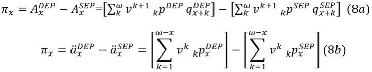
In the light of this consideration, we aim to calculate the effective dependency premium of an insurance product. We suggest a general and flexible formulation for detecting the dependency premium in order to provide an approach with wide practical applications for handling portfolio heterogeneity. For each population, the dependency premium π is quantified as the spread between the premium calculated by considering dependent forecasts and that calculated by considering separate forecasts, as in formulae (8) below. In particular,
contracts; for example, in the case of a whole life insurance or a life annuity the dependence premium would be
=[∑ ] [∑ ] ( ) ̈ ̈ [∑ ] [∑ ] ( )
where according to the standard actuarial notation v1/(1r) and r is the interest rate,
is the survival probability after kyears, is the probability of death for an insured
[image:6.595.127.489.129.199.2]aged x between ages xk and xk1, is the final age considered in the mortality
table. The survival and mortality probabilities are selected taking the central projection of mortality rates; more prudential choices can be easily introduced depending on the scope of the analysis.
The framework that we propose enables us to quantify the differential in the premiums, reserves and other key actuarial quantities.
Corollary. In the risk management of a heterogeneous portfolio, a reduction of the premium may be obtained from the “diversification” effect due to the dependence structure between sub-groups of the population. In other words, if the premium reduction were passed on to the policyholder, he/she would be able to take advantage of the “diversification” of the populations in the insurer’s portfolio that are characterized by the dependence structure.
3. Numerical Illustration
In this section, some empirical evidence is provided to illustrate our methodology. The analysis is performed on two sub-groups, male and female, of the Italian population for ages 0 up to 100, using observations for the historical window of 1982-2012. The projections are developed for the future time horizon from 2013 to 2033. The investigation compares the common forecasts obtained through the model and the separate ones obtained by the application to the dataset of the LC model.
The steps of the fitting procedure are the following:
a) We fit the LC model to the whole group and find B(X) and K(t) b) We fit the LC model to each sub-group i and find a(x,i)
c) For each sub-group i we derive the residual matrix of the common factor model Mi= log(m(x,t,i,))-a(x,i)-B(x)K(t)
d) For each population i we apply the SVD to Mi and obtain bj(x,i)K(t,i) from the first j orthogonal vectors.
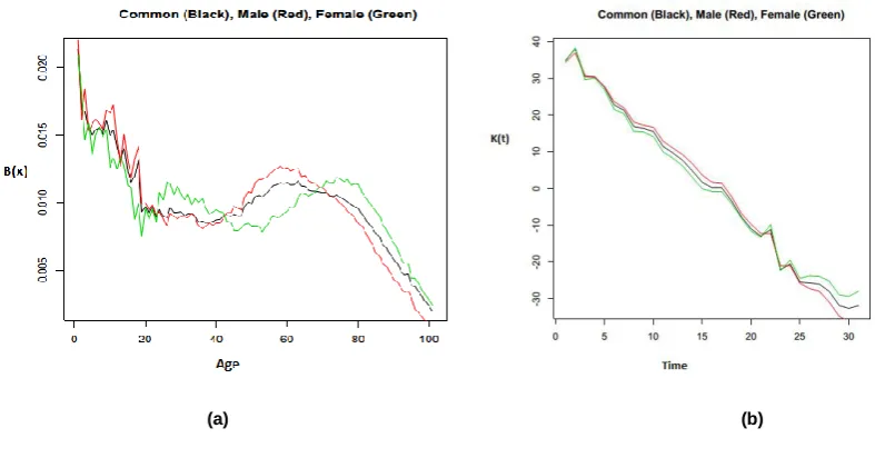
Figure 1 represents the common factors B(x) and K(t) in black and also the parameters
) (x
Kleinow and Richards (2016) show that ARIMA models better represent the trend of mortality time series than simple random work process and implement bootstrap techniques to measure uncertainty in the estimation of parameters. However, in this research, uncertainty in the model parameters is not taken into account.
In order to fit an ARIMA(p,d,q) model for each time series, we compare the AIC values for different value of p,d and q; the results and the fitted parameters are shown in Table 1.
AIC ARIMA(1,0,0) ARIMA(1,1,0) ARIMA(1,1,1) ARIMA(1,1,2) Parameters
Common 177.23 165.22 167.39 147.09 Ar1 0.99 Intercept 1.36
Male -63.27 -63.72 -62.42 -60.82 Ar1 0.10
Female -61.95 -61.53 -60.04 -59.40 Ar1 0.90 Intercept -0.09
Table 1 –AIC and parameters of the ARIMA models
Figure 2 shows the common projected trend (black line): it is an average of the lower male projected trend (red) and the higher female projected trend (green). This is due to the fact that the historical mortality trend was more downward for females than males (see Figure 2), but, since the year 2000, males have experienced a greater reduction in their mortality trend. For this reason, the gap between males and females considered separately appears widened, while if we consider just the common trend we average the effect of the greater mortality reduction for males and the smaller reduction for females. Figure 3 shows the consequences for the life expectancy at birth calculated on a period basis with the common model or separately; life expectancy at birth is defined as how long, on average, a newborn can expect to live, if current death rates do not change.
(a) (b)
[image:7.595.91.485.486.692.2]Figure 2 – Forecasting of the Kt parameter on Italian Population, CM and LC for male and female
<
(a) (b)
Figure 3 – Coherent by CM and Separate by LC Forecasts of the life expectancy at age x=0, Male (a), Female (b)
[image:8.595.183.435.92.339.2] [image:8.595.123.476.368.545.2]
(a) (b) (c) (d)
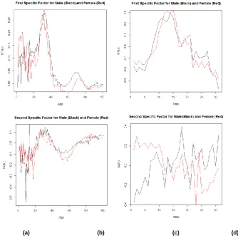
Figure 4 – First and Second Specific Factors by MM respectively from top on left (a), (b) to bottom on the right (c), (d)
Figure 4 plots the evolution of the specific factors of the parameters of the MM, where the differences between the results for males and females are more evident. In this application we have chosen to fit two specific components based on the empirical valuation of the dataset, trying to balance the need for a parsimonious model and a representative one.
Tables 2a and 2b show the explanation ratios and the AIC for the CM, AM and MM. The outcomes reveal that the MM provides a better performance in terms of goodness of fit.
EXPLANATION RATIO COMMON AUGMENTED MULTI
FACTOR MODEL
Male 0.82 0.86 0.88
[image:9.595.138.473.77.411.2]Female 0.80 0.83 0.86
Table 2 a–Explanation Ratios of the common, augmented and factor models AKAIKE INFORMATION
CRITERION COMMON
AUGMENTED MULTI
FACTOR MODEL
Male -13354.12 -13941.45 -14293.46
[image:9.595.58.519.582.779.2]Table 2b–AIC of the common, augmented and multifactor models
The second step of our application consists in verifying whether the considered models provide plausible forecasts. The backtesting procedure considers what results would have been produced if the model had been used in the past and can be used to evaluate the ex-post forecasting performance of the mortality models. Thus, Lee and Miller (2001) evaluate the performance of the LC model by examining the behaviour of the forecast errors. In order to implement a backtesting procedure, it is necessary to select the metric of interest, such as the mortality rate, the life expectancy, the prices of annuities and so on, depending on the purpose of the analysis. Since our aim is to investigate the feasibility of different mortality models, we focus on the projections of the mortality rate itself. Once we have chosen the metrics, we have to select the historical ‘lookback’ window and the forecast horizon over which forecasts are made. Wang and Liu (2010) highlight that, as the fitted period changes, models that perform better, may also change. In the present paper, we focus on long time horizon forecasts, because the performance of pension plans and life insurance companies are principally influenced by the accuracy of these long term forecasts. In particular, we fit the models from 1982 to 2002, thereby using a 20 year in-sample period, then we project the mortality rates from 2003 to 2013 and compare projections with the observed rates. The projections are derived considering only the evolution of kt: errors in ax and bx are ignored. The empirical justification is found in Lee and Carter (1992); they show that the standard errors of ax and bx become less significant over the forecast time in comparison to the standard error of kt and find that the 98 per cent of the standard error of forecasted US life expectancy at birth was accounted for by the uncertainty in kt .
(a) (b)
Figure 5– Mean Absolute Forecast Error for Male (a) and Female (b)
(a) (b)
Figure 6– Mean Forecast Error for Male (a) and Female (b)
(a) (b)
Finally, we use the mortality projections derived from the models presented to price some key life insurance products and calculate the dependency premium (along the lines of equation (8)) in a heterogeneous portfolio composed of males and females. Tables 3 and 4 report the results
for the actuarial calculations for the single premiums for a pure endowment and whole life insurance policy for a male and female policyholder in the case of the separated and MM forecasts. In the pure endowment contract, the value of the benefits increases if the insured lives longer; for this reason the premium paid by female is higher if we consider the separate projections than the MM model projections. In order to offer a wider evaluation of the issue, we calculate also the single premium for a pure endowment for males and females in the case of CM: in this case the dependency premium for male and female is equal to -0.15 and +0.06. Even if the difference with respect to the dependency premium calculated through the MM is not so large, the impact on the whole insurance portfolio can be important.
For the whole life insurance contract, the value of the benefits decreases if the insured lives longer and the results are reversed.
Tables 5a and 5b show respectively the single premium for an immediate and a deferred life annuity: since in the separate model female have a lower life expectancy, the price of the annuity appears lower than in the case of the MM model.
The resulting values of the dependency premiums suggest a potential diversification effect in a heterogeneous portfolio. The results have to be applied in light of the European Council Directive 2004/113, the so called “Gender Directive”, implementing the principle of equal treatment between men and women in the access to and supply of goods and services. While previously, the use of gender based actuarial factors was permitted, the Directive obliged insurance companies in Member States to calculate premiums and benefits on a unisex basis. In the case of a portfolio composed by both males and females, the premiums required have to be calculated as a weighted average of the single premiums of each subpopulation; taking into account dependence it is possible to obtain a well-balanced unisex premium and, potentially, one that is more competitive than that calculated without dependence.
PRICE SEPARATED MULTIFACTOR
MODEL
Male 9.99 9.82
Female 10.08 10.15
Dependency Premium
Male -0.17
[image:12.595.169.426.540.720.2]Female +0.07
Table 3– Pure endowment , with payment R=1,000, insured aged x=30, duration n=35, r=0.05
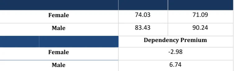
PRICE SEPARATED MULTI
Female 74.03 71.09
Male 83.43 90.24
Dependency Premium
Female -2.98
Male 6.74
Table 4 a – WholeLife Insurance, R=1,000, x=30, r=0.05
PRICE SEPARATED
MULTI FACTOR MODEL
Female 182.58 175.83
Male 202.90 217.52
Dependency Premium
Female -6.75
Male 14.62
Table 4 b – WholeLife Insurance, R=1,000, x=50, r=0.05
PRICE SEPARATED
MULTI FACTOR MODEL
Female 1709.48 1722.74
Male 1670.28 1639.79
Dependency Premium
Female 13.26
Male -30.49
Table 5a – Life Annuity, R=100, x=50, r=0.05
PRICE SEPARATED
MULTI FACTOR MODEL
Female 904.98 917.33
Male 866.41 838.05
Dependency Premium
Female 12.36
Male -28.35
[image:13.595.110.487.74.188.2] [image:13.595.109.491.224.467.2] [image:13.595.110.488.583.744.2]Finally,in order to offer a wider evaluation of the issue, we calculate also the single premium for a pure endowment for males and females in the case of CM: in this case the dependency premium for male and female is equal to -0.15 and +0.06. We highlight that, even if the difference with respect to the dependency premium calculated through the MM is not large, the impact on the whole insurance portfolio could be important. Similar calculations can be carried out for the other contracts.
4. Conclusions
The life expectancy of given sub-populations in an insurance portfolio can show a similar trend over time; taking into account the dependence could improve the calculation of the fair price of the insurance products. The calculation of the dependency premium could produce positive effects in terms of the reduction of price for some subgroups. The insurers or pension fund managers could take advantage in terms of risk diversification in a portfolio with populations which show a similar trend but negatively correlated specific effects. In light of these considerations, we propose a flexible multifactor model set-up for measuring the dependency premium by introducing specific factors in a general scheme for the dependence structure in the mortality data. The model is supported by diagnostic analysis and enriched by several comparisons. In particular, our findings appear to suggest a possible portfolio diversification for subgroups of policyholders defined by type of insurance policy – this effect arises from the differences in the gradient of improvements over time in mortality and life expectancy across the sub-groups.
Further research will be developed on the comparison of other typical portfolio subgroups with a particular emphasis on longevity basis risk.
References
Cairns A.J.G., Blake D., Dowd K., 2006, A two-factor model for stochastic mortality with parameter uncertainty: Theory and calibration, Journal of Risk and Insurance, 73: 687-718.
D’Amato V., Haberman S., Piscopo G., Russolillo M., 2012, Modelling dependent data for longevity projections, Insurance: Mathematics and Economics. 51, 694–701.
D’Amato V., Haberman S., Piscopo G., Russolillo M., Trapani L., 2014a, Detecting common longevity trends by a multiple population approach, North American Actuarial Journal 18,139–149.
D’Amato V., Haberman S., Piscopo G., Russolillo M., 2014b, Computational Framework for Longevity Risk Management, Computational Management Science, vol.11(1), p.111-137
Dowd K., Cairns A., Blake D., Coughlan G., Khalaf-Allah M., 2011, A gravity model of mortality rates for two related populations, North American Actuarial Journal 15, n. 2.
Jevtic, P. and L. Regis, A continuous- time stochastic model for the mortality surface of multiple populations, EIC Working Paper 3/2016.
Kleinow T., Richards S.J. 2016. Parameter risk in time series mortality forecasts. Scandinavian Actuarial Journal. To appear
Lee R., Carter L., 1992, Modelling and Forecasting U.S. Mortality, Journal of the American Statistical Association, 87, 659-671.
Li N., Lee R., 2005, Coherent mortality forecasts for a group of populations: An extension of the Lee–Carter method, Demography 42(3),575–594.
Plat R., 2009, On stochastic mortality modeling, Insurance: Mathematics and Economics 45, 393-404
Renshaw A.E., Haberman S., 2006, A cohort-based extension to the Lee- Carter model for mortality reduction factors, Insurance: Mathematics and Economics, 38: 556-570.
Villegas A., Haberman S., Kaishev V., Millossovich P., 2017, A comparison of two population models for the assessment of basis risk in longevity hedges, ASTIN Bulletin, To appear.