City, University of London Institutional Repository
Citation:
Broom, M. and Cannings, C. (2017). Game theoretical modelling of a
dynamically evolving network I: general target sequences. Journal of Dynamics and Games,
4(4), pp. 285-318. doi: 10.3934/jdg.2017016
This is the accepted version of the paper.
This version of the publication may differ from the final published
version.
Permanent repository link:
http://openaccess.city.ac.uk/17808/
Link to published version:
http://dx.doi.org/10.3934/jdg.2017016
Copyright and reuse: City Research Online aims to make research
outputs of City, University of London available to a wider audience.
Copyright and Moral Rights remain with the author(s) and/or copyright
holders. URLs from City Research Online may be freely distributed and
linked to.
NETWORK I: GENERAL TARGET SEQUENCES
M. Broom1,∗ and C. Cannings2 1
Department of Mathematics, City, University of London, Northampton Square, London EC1V 0HB, UK.
School of Mathematics and Statistics, The University of Sheffield, Hounsfield Road, Sheffield, S3 7RH, UK.
[email protected] *corresponding author
Abstract. Animal (and human) populations contain a finite number of individuals with social
and geographical relationships which evolve over time, at least in part dependent upon the actions of members of the population. These actions are often not random, but chosen strategically. In this paper we introduce a game-theoretical model of a population where the individuals have an optimal level of social engagement, and form or break social relationships strategically to obtain the correct level. This builds on previous work where individuals tried to optimise their number of connections by forming or breaking random links; the difference being that here we introduce a truly game-theoretic version where they can choose which specific links to form/break. This is more realistic and makes a significant difference to the model, one consequence of which is that the analysis is much more complicated. We prove some general results and then consider a single example in depth.
Keywords degree preferences; graphic sequences; Markov process; stationary distribution; Nash equilibrium.
1. Introduction
1.1. Modelling populations. When modelling biological populations, inevitably many simplifi-cations are made. Until recently, most evolutionary models (e.g. [19, 20, 21, 30, 31, 25, 26]) have considered an infinite well-mixed population where all individuals interact. Whilst the assumption of infinite size can often be reasonable, there are also important differences between finite and infinite populations, and important work on finite populations includes the classical mathematical genetic models of [16] and [52], as well as the evolutionary game model of [48].
Real populations are also not homogeneous, containing a population structure, and this has been incorporated in various ways. Models incorporating such structure include genetic models based upon a number of sub-populations [53, 27, 33, 10], and more general models of evolution on a graph originating with [28] and discussed in Section 1.2. Here we consider a model introduced in [6] in which ”evolution” takes place on the class of graphs with a fixed number of vertices, the set of edges changing according to choices made by the vertices. Details are given in Section 1.3.
1.2. Background Literature. A simple graph G= (V, E) is a set of vertices and a set of un-ordered pairsE⊆V ∗V with (i, i)∈/E. Vertices are considered indistinguishable if they have no special type over and above properties resulting from the graph itself, e.g. degree. When consid-ering some evolutionary process for graphs where vertices represent individuals and the edges are links there are several levels of complexity, depending on whether the vertices are distinguishable, whether the edges are fixed, whether the numbers of vertices and or edges changes. There can be various dependencies between the vertices and edges.
It is often desired to generate a random sample of members of some class of graphs. For example, one would like to generate elements of the set of r-regular-graphs onn nodes. Here the vertices are indistinguishable and the number of vertices fixed. Discussion of this can be found in [4]. In [3] the graph at some timetgrew by the addition of vertices and edges. New vertices were added one at a time, the one added at timet+ 1 was linked to some ”c” of those at timet, these latter vertices being chosen with probabilities proportional to the degrees of the vertices at timet. This gives rise to a power law distribution of degrees, see [5] for rigourous derivations.
A third possibility is that the graph grows by some reproductive process. Graph theory has introduced a number of products which form a new graph from two earlier ones. For exam-ple, the Tensor product of graphs G(V, E) and H(W, F) is the graph M = (V ∗W, G) where ((v1, w1),(v2, w2))∈G, if, and only if, (v1, v2)∈E and (w1, w2)∈F. Another approach is that of [44, 45, 46]. In their model each vertex at time t produces an “offspring”,current edges are retained and then edges are formed between the vertices at t and those at time t+ 1 according to some rule. This process grows indefinitely, and the authors track various properties such as chromatic number and diameter through time.
In contrast to the models above, the vertices may possess a type, which may change during time. In many of these latter models there are two types in the population (resident and mutant),and the state of the population, the set of mutant individuals, say, evolves according to an evolutionary dynamics. As per Moran’s [33] model individuals are selected, according to some fitness dependent on type, and they replace one of their neighbours chosen at random. The most important feature of such populations is the fixation probability, the probability that a randomly placed mutant will eventually replace the resident population [2, 9].
We note that for real populations both of these features change, and there has been much research considering the way in which the interactions of the individuals at the vertices affect not only their type but also the structure of the network, see for example [47]. The growth and structure of the graph can be dictated by an evolutionary game, and in particular by the prior interactions of individuals, as in [36, 37]. Here links are formed or broken at rates which depend upon the types of the individuals, and the authors consider an evolving population where evolutionary dynamics happen on a slower timescale than the linking dynamics. Alternatively [43] considered various dynamic models of network formation assuming reinforcement learning. A model where it is not past interactions but reputation that influences structure is given by [17], and one where prosperity influences the structure is given in [12]. A good review of work in this area up to 2010 is given in [39], while a more recent but less specific review is in [1]. An example of more recent work is [40] who discussed such co-evolutionary models examining the prisoner’s dilemma and the snowdrift game, together with the Birth-Death process. As stated in [1], while the details of the above models vary, a common theme to many is that cooperative behaviour is easier to achieve when cooperators can group themselves together and exclude defectors effectively.
does not change since there is no birth or death of individuals, but the connections between in-dividuals will change according to their preferences and strategic decisions. The emphasis of our papers is the evolution of the structure itself, and although there may be many types of individuals (a type being its targeted number of neighbours) our process is thus not co-evolutionary, as the types do not change. Our process could be considered as a detailed examination of a snapshot in evolutionary time of a more complicated version of the type of model from [36, 37], and it would be possible to embed our model into such an evolutionary scenario.
The kind of networks that we consider arise naturally in many contexts including in biology, economics and sociology, and this is the subject of a lot of recent research interest. Example networks are companies which trade with each other in economics, individuals who are friends in sociology or the owners of neighbouring territories or food webs ([15]) in biology. In social animals there are dominance and mutualist interactions and, for example, primate social structures can be complex and influence key behaviours such as the level of cooperation ([49, 50]).
Populations can also change in important ways over short periods of time. A population of animals may contain individuals with different degress of desire to interact with others. This phenomenon is called “sociability” and has been investigated in various species. Examples of such differences include (non-human) primates [11], bottlenose dolphins [51], [13] and sheep, where different indi-viduals differ in how close they want to be to other flock members [42].
In these examples there are temporary links between individuals. The probability of a link existing between a pair of individuals will in reality often be affected by the relatedness of those individuals, by their genders, by dominance relationships or by spatial factors. In the bottlenose dolphin case the links are reciprocal, whereas in others they might be initiated, or broken, by the action of one individual only. Similarly the absence of a connection may benefit one but not the other (for example a female and a poor quality male). An important related area of research is that concerning biological markets and partner choice [34, 35].
In this paper we do not model such complex behaviours, but simply the network of interactions. Individuals (vertices) in our networks are distinguishable only by the number of links they would like to form with others. Each individual will want to make changes which improves its number of links, but since all links involve two individuals, the actions of others can make an individual’s situation worse. The key difference with previous work [6] is that individuals will not just choose a random action which improves their situation in the short term, but will strategically choose which individuals are best to link to/ break from. As we shall see, this makes the situation much more complex.
1.3. A dynamic network population model. In [6] we considered a population of individuals represented by the setV ={1,2, . . . , n}and the simple graphG= (V,X) whereX= (xij)i6=j=1,...n
described the links/edges between pairs of individuals withxij = 1 if there is a link and xij = 0
otherwise. In particular we considered a random process in discrete time on the evolving edge set
Xt= (xij,t)i,j=1,...n, where the subscripttindicates that this is the edge set at timet. Throughout
the paper we shall use the same terminology, but we shall often drop the subscript t when we describe features of the process that are not time-dependent and this causes no ambiguity. In [7] we investigated the possible paths and end states of the process. We describe the process below. At any given time t individual i had a number of edges ei,t to other individuals, and the vector
et= (e1,t, e2,t, . . . , en,t) was referred to as thesequence et.
mi ≤Mi≤n−1. In much of the workmi=Mi =ti, withti denoted as the unique target of i,
and this is the situation in the current paper.
If i was selected with ei < mi (such a vertex is referred to as a Joiner) then it formed a new
edge, connecting to one of the other vertices it was not connected to at random. If ei > Mi (a
Breaker) then it broke one of its edges at random. Otherwise, it neither created nor broke an edge (a Neutral vertex).
At successive time points, a vertex was chosen at random, withi being selected with probability
pi > 0, and an edge (potentially) changed following the above, yielding a homogeneous Markov
chain.
The transitions at timetdepended upontonly through the state, i.e. the process was homogeneous, and were defined as follows:
1) For anyx∗ which differs fromxin a single entry, wherexij = 0, x∗ij = 1 for somei, j,
P(Xt+1=x∗|Xt=x) =
pin−11−e
i +pj
1
n−1−ej ei< mi, ej< mj pin−11−e
i ei< mi, ej≥mj pjn−11−ej ei≥mi, ej< mj
0 ei≥mi, ej≥mj.
2) For anyx∗ which differs byxin a single entry, wherexij= 1, x∗ij= 0 for somei, j,
P(Xt+1=x∗|Xt =x) =
pie1
i +pj
1
ej ei> Mi, ej> Mj pie1
i ei> Mi, ej≤Mj pje1j ei≤Mi, ej> Mj
0 ei≤Mi, ej≤Mj.
3) Similarly for any otherx∗, differing fromxin two or more entries,
P(Xt+1=x∗|Xt =x) = 0.
The probability of the sequence being unchanged is simply 1 minus the sum of the above proba-bilities.
2. An Overview
2.1. A brief synopsis of previous papers[6]and[7]. In [7] we studied graph theoretic aspects. We give a brief outline here in order to inform the current work. We introduced the notions of the deviation of a graph from a given target and the score of a sequence.
Definition 1Thedeviationof individual/vertexiis denoted asi,t= max[(mi−ei,t),(ei,t−Mi),0],
and the deviation of the above graph Xt is defined as the sum of the vertex deviations, Υt =
P
i=1,ni,t.
Definition 2 There is clearly a minimum value of the deviation for any given collection of the ranges [mi, Mi], and this is termed thescore.
If the score is 0 the sequence is calledgraphicand there is a lot of work on such sequences, see for example [22],[18],[23],[32],[41].
is always a path of allowable moves enabling the process to reach a member of the minimal set,
K(min). Since the process could never increase the deviation of the graph, onceJ(min)/K(min) is reached, that set cannot be left. It was proved that for non-graphic sequences K(min) was connected, so that the process always converged to a unique closed set of states. Note that this is not true for graphic sequences, where|J(min)|= 1 but K(min) will often have more than one element (e.g. for (1, 1, 1, 1) we have|K(min) = 3|), since once the mimimal set is reached there will be no transitions, so no pair of elements ofK(min) are connected. Finally in [7] we demonstrated how to find the score of any sequence using a modified Havel-Hakami algorithm [18],[23], and how to find all members ofK(min) (and henceJ(min)) using the methodology of Ruch-Gutman [41]. In [6] we considered the Markov chain itself. We considered the Markov chain overK(min), since all states not in this set will be transient following the above. We showed that the process was reversible and so in detailed balance, which thus yielded a unique stationary distribution over
K(min). We then demonstrated a method to find this stationary distribution.
We considered some specific classes of sequence, in particular arithmetic sequences and all or
nothingsequences, and in particular gave a form for the stationary distribution of the latter for an
arbitrary number of vertices. We revisit the former in the current paper.
2.2. Current and Future Work. The current paper considers detailed aspects of the structure ofK(min). In [7] we proved certain restrictions to exist on the its elements, e.g. that for any such graph we know that all Joiners (that is vertices have degree less than their target) must be joined. Here we extend such analysis to consider the possible sequences of Joiners, Breakers (vertices with degrees greater than their target), and Neutrals (the remaining vertices) through time. Vertices fall into four classes; those which are always neutral, those which are never Joiners, those never Breakers, and those which can be either Joiners or Breakers. We specify rules regarding the possible sequences of class memberships of the vertices as we move through the monotone decreasing of targets.
We then consider a model, which in contrast to those of [6] and [7] considers the possibility that the individual at a vertex may choose between the available possibilities according to some aspect of the future costs at that vertex. We have chosen to consider the case where an individual is capable of calculating the stationary distribution which will result from various changes. We discuss various criteria for switching including some where an increase in costs is possible. For systems where the calculation of the stationary distribution is not reasonable we introduce two threshold models, basing their decision on a recent sequence of states.
In Section 5 we consider a specific example (target {4,3,2,1,0}) calculating for each of the 64 strategy combinations over the minimal set, the payoff for each possible switch. We consider cases where a switch can only occur if there is a cost lower than the current one, cases where switches are possible when the cost is no bigger, and cases where there is a cost incurred in switching. We identify multiple pure Nash equilibria.
We consider two models which do not require the evaluation of the stationary distribution, rather being based on estimates from recently visited states, and thresholds for switching. These show different behaviour to the full model.
A number of questions have been left open here. We have discussed in detail but not resolved the question of what can occur under non-strict moves, i.e. those which allow individuals not to make their deviation as small as possible at every opportunity.
latter in particular is complicated and hard to deal with in generality, and so we have restricted ourselves to considering one example in detail, and demonstrating the important concepts to con-sider in any more extensive analysis. From this paper we see this complexity, but also that strategic choices lead to clearly different results than the simply random process from [6].
We shall discuss in a subsequent paper [8] certain classes of targets, especially those with score 1. These are the closest sequences to graphical sequences, and yield certain simplifications that will make them more amenabe to analysis. This will also involve the consideration of cases with mixed Nash equilibria.
3. A strategic model
In the model from Section 1.3 each individual has a target number of links, specified by the vector
t. The graph updates through a two stage process, where a random individual is selected to update its links, and if it is below (above) its target number of links, it picks a random link to form (break). There is no strategic element to this process, which evolves as a Markov chain.
However, it may be that it is advantageous to form/break some links rather than others. For example it would be better to form a link that is less likely to be immediately re-broken, either because the change made is for mutual benefit or because the individual linked to would be likely to break another link when given the choice (through its own preference, or if it has many links that it can break).
3.1. Strategies. The population state is denoted by the edge setXas before. In each state any individual can be selected to change one of their edges. They have ndistinct (pure) choices, to change their edge to any of the othern−1 individuals, or to make no change. We shall denote the probability that individualichooses to change edgexij, conditional onibeing selected to make the
change, byuij, withuii denoting the probability that no change is made. We have the following
pure strategies: individual i chooses to change edge xij is denoted byuij = 1, and i making no
change is denoted byuii = 1. Thus we can write all selected changes in the form of a matrixU,
withUhaving row sums equal to 1.
The strategy matrixUdepends upon the stateX, and so the full set of strategies of the population is denoted byUX(similarly its elements byuij(X)), where the strategy of individualiis represented
by the set of ith rows of this collection of matrices. For any x∗ which differs from x in a single
entry, wherexij= 0, x∗ij = 1 orxij= 1, x∗ij= 0 for a giveni, j,
(1) P(Xt+1=x∗|Xt=x) =
uij(X)+uji(X)
n .
Individuals which were rational but could only see the immediate consequences of any changes would follow the strict system, and it seems logical that real systems would often follows these rules. One consequence of following the strict system is that the score cannot increase. Thus for the strict system,uij= 0 wheneverxij = 0, ei≥ti orxij = 1, ei ≤ti, as this change would involve
a worsening move. The simple “strategies” used in [6] are consistent with the strict system, for example If we allow non-strict moves, our analysis can be significantly complicated, as we see later in Section 3.
3.2. Payoffs. Individuals want to minimise their deviation, and we shall denote their payoff as the negative of their expected long term deviation. In particular, if a process with individuals following strategies UX has a unique stationary distribution overX, denoted by π(X), then the
payoff to individuali is
(2) Ri(UX) =−
X
X
i(X)π(X),
wherei(X) is the deviation ofiin stateX.
3.3. Stability and strategy switches. Individuals can try to improve their payoffs by changing their strategy. We consider two types of strategic changes;
Local changes- individualichanges theith row ofUX for a single stateXonly;
Global changes- individuali changes theith row ofUX for any number of states simultaneously.
Making such global changes might be advantageous, since any individual change would potentially affect a number of the probabilities of occupying particular states/ taking particular paths, which then may alter the best choices elsewhere. This would depend upon a significant ability to calculate, and so it may be reasonable to assume that it is not possible for individuals to make such global changes. An individual with limited cognitive powers might, for example, only use strict moves and local changes.
Only changes by a single individual at a time are allowed. We shall say that an individuali plays
optimally if under all allowable changes UX → UiX (including no change) it chooses a strategy
which achieves maxiRi(UiX). A strategy set is a Nash equilibrium under local or global changes
if, under all allowable changes byi:UX→UiX
(3) Ri(U)≥Ri(Ui) i= 1, . . . , n.
In this section we briefly consider the process not restricted to the mimimal set K(min), strict moves or neither.
3.4. The strict system on the non-minimal set. For non-strict moves, and allowing individ-uals to play sub-optimally (where optimal play is as described above), clearly the process does not possess the nice properties from [6] and [7]. The process does not necessarily converge to the minimum set, or have a unique stationary distribution. If individuals are allowed to remain on the same deviation when there is an opportunity to improve, then the strategy of all individuals making no changes in any circumstances will clearly not lead to the minimum set, for example. Clearly for any non-graphic sequence the target can never be achieved, and so there is always at least one individual that is not achieving their target. Given that the targets are all between 0 and
following example shows that even with strict (but not necessarily optimal) play the minimal set may not be reached.
Example 1 Consider the case where vertices A and C have target 1, B and D have target 0. Suppose currently neither of A and B is linked to either of C and D. When A has no links, the strict system means that it must form a link when selected. Suppose that it always links to B. Similarly, assume that C always links to D when its score is 0. B and D will simply break the link that they have (unless they have more than one which can never occur following the above) and so the system will simply consist of two pairs A and B, C and D, repeatedly breaking and forming links, with a score of 2. The minimal set consists of the single graph with the single link A to C, which will never be reached.
However, we are principally interested in what happens when optimal play is employed by individ-uals, and so we shall restrict ourselves to finding Nash equilibria of our system. Note that we have not shown whether it is possible to have Nash equilibria that are not in the minimal set. This is a difficult open problem; we conjecture that it is possible to have such equilibria, but that it requires a sufficiently large number of individuals with a sequence of high score.
3.5. The non-strict system. Considering Example 1 above, we shall now show that it is possible for non-strict moves to be optimal under certain circumstances.
Example 1 Cont. Consider again the case where vertices A and C have target 1, B and D have target 0. Assume that B,C,D always play strictly (i.e. reduce their deviation when they can, and do nothing when they are on target) and that B will always split from A as its first choice move, D will always split from C as its first choice, and C will always link to D as its first choice, similarly to before. Then if A always links to B as its first choice, we obtain the situation where all fol-low legal strict moves but the unique minimal graph is never reached and the payoff for each is 1/2. Suppose that A is faced with the situation where it is connected to B, but C and D are split. What if it chooses to link to C? This is a non-strict move as it is currently achieving target. However, if it does this, if C and D are picked next, they will do nothing (we assumed they always behave strictly, and they are now on target). Either A (assuming it plays as previously described except in the original case) or B will split A-B, which will lead straight to achieving the target for all (in an expected time of 2 moves). Thus here is an example where non-strict play is optimal.
Note an alternative in the initial situation would be to wait until B breaks from A and then link to C as the next opportunity, but this would mean a sub-optimal decision was made at the original decision; also it would take at least twice as long to reach the minimal graph (A would have to be picked with mean time 4, and only then would the final target have been achieved if C has not linked to D in the meantime).
4. The strict system on the mimimal set
We now consider processes restricted to the strict system acting onK(min). We define the matrix
A= (akl) as the matrix of transtions on the elements of K(min), such thatakl is the probability
of moving from the minimum graph stateXk toXl, i.e.
(4) akl=P(Xt+1=xl|Xt=xk),
using equation (1). Thus given a choice of strategiesUX that lead toK(min) there is a unique
matrixA. We can (and will) consider alternative strategy combinationsUX, leading to different
matricesA.
This will, in general, greatly reduce the number of transitions that need to be made. For example, if n = 5, X has 210 elements, each yielding a potentially different 5×5 matrix, giving 25600
transition parameters to consider. In Example 3K(min) contains 8 elements and so at most 64 potential transitions, only 28 of which are non-zero.
We know from Theorem 5 from [7] that K(min) contains at least one element with no Joiners, and at least one element with no Breakers. Thus no vertex is always a Breaker, and no vertex is always a Joiner. K(min) is connected (unless the target sequence is graphic, when all vertices are neutral), and so no vertex is sometimes a Joiner and sometimes a Breaker but never Neutral. Thus every vertex is Neutral for some elements ofK(min), and we have the following:
For the setK(min) associated with any target sequence, we can divide the individuals (vertices) into four classes:
a) Those which are sometimes a Joiner and sometimes a Breaker (and also necessarily a Neutral) for some elements ofK(min); these individuals constitute the setSA,
b) those which are Joiners (or Neutrals) for some elements but never Breakers; the setSJ,
c) those which are Breakers (or Neutrals) for some elements but never Joiners; the setSB,
d) those which are always Neutral; the setSN .
Clearly, since any graphical sequence has deviation zero, it will only have individuals of type d). For non-graphical sequences, sinceK(min) contains elements with Joiners and elements with Breakers, it must contain either individuals of type a) (and possibly some of type b) and/or c) as well), or if there are no type a)’s there must be individuals of types b) and c).
Lemma 1. We cannot have individuals of type a) and individuals of type d) for the same sequence.
Proof: Suppose that we have an individual of type d). It is always Neutral, so its set of links do
not change. It cannot be joined to any Breaker, as breaking that link would leave the graph in
K(min), but change the vertex to a Joiner. Similarly it cannot be split from any Joiner, as forming that link would leave the graph in K(min), but change the vertex to a Breaker. Any vertex of type a) will be a Joiner at some times and so joined to the original vertex, but a Breaker at other times, and so split from it. Thus there can be no such vertex.
Lemma 2. Suppose we have a target t = {t1, t2, . . . , tn} on a set of vertices 1,2. . . , n where
SJ ={t1, t2, . . . tu},SN ={tu+1, . . . , tv}, andSB ={tv+1, . . . , tn}.
(i) We shall now introduce an extra vertex. For any set{wu+1, wu+2, . . . , wv}such thatwi ∈ {0,1},
t0 ={t1+1, t2+1, . . . , tu+1, tu+1+wu+1, tu+2+wu+2, . . . , tv+wv, tv+1, tv+2, . . . , tn, u+P v
i=u+1wi}
will have precisely the same transition graph as t={t1, t2, . . . , tn}, in the sense that if two states
are joined in the original graph then the augmented states will be joined in the transition graph of the augmented target, where the new vertex will be in class d).
(ii) We shall now “remove” vertexu+ 1. For any set {wu+2, wu+3, . . . , wv} such thatwi ∈ {0,1},
t00 ={t1−1, t2−1, . . . , tu−1, tu+2−wu+2, tu+3−wu+3, . . . , tv−wv, tv+1, tv+2, . . . , tn}will have
Proof: (i) Consider a graph with the original targett. Add a new vertex and link it to all elements in SJ, split it from all elements in SB, and link it to any given element i of SN if and only if
wi = 1. The new vertex will be a Neutral, and every individual will have the same deviation
(and in the same direction) as the original graph. For the given choices of the wi’s, there is a
1-1 correspondence between the set of original graphs and the set of transformed graphs; the only difference is the presence of the new vertex. But this vertex is split from all vertices that can ever be Breakers and joined to all that can be Joiners, and so its deviation will never change, i.e. it is an element ofSN.
(ii) Similarly, let us remove an element of SN. As stated in the proof of Lemma 1, this vertex
must be split from all vertices that can be Breakers, i.e. SB, and joined to all elements that can be
Joiners, i.e. SJ. This means that removing this vertex will take one from the links of all elements
of SJ and none from all elements ofSB. It will take a link away from an element ofSN if there
exists one, and so this will determine the values of wi fori ∈SN which keeps the deviations the
same (note that an element ofSN has the same links to all other elements ofSN for all elements
of K(min), so we have the same set of wis for all graphs). Thus again we have a one-to-one
correspondence between the two minimal sets.
Thus from Lemma 2, if we have individuals of types b), c) and d) then we can effectively add or remove as many elements of type d) as possible without changing the minimal set at all. This leads us to the following result.
Theorem 1. Suppose we have a targett={t1, t2, . . . , tn}whereSJ ={t1, . . . , tl},SB={tl+1, . . . , tn}
and so SN =φ. Now suppose we have a graph G ={V, E} where V ={vn+1, vn+2, . . . , vn+m},
and the degree of vi ∈ G is di. Then by Lemma 2 the target t
0
= {t1 +m, t2 +m, . . . , tl+
m, tl+1, tl+2, . . . , tn, dn+1+l, dn+2+l, . . . , dn+m+l}has precisely the same transition matrix as t.
Thus for any target t0 of the same type ast i.e. only elements in SJ and SB, there is a set of
targets whose transition graphs are isomorphic to the transition graph oft.
Example 2. Ift={3,2,1,0}, sol = (n−2) = 2 then for m= 0 we have{3,2,1,0}, for m= 1,
{4,3,2,1,0}, for m = 2, {5,4,2,2,1,0} and {5,4,3,3,1,0}, and for m = 3 ,{6,5,2,2,2,1,0},
{6,5,3,3,2,1,0},{6,5,4,3,3,1,0}and{6,5,4,4,4,1,0}. Note that the Breakers have been moved to the end of the target to give a non-decreasing sequence. The target{4,3,2,1,0} is treated in some detail later.
Theorem 2. Suppose we have a target t = {t1, t2, . . . , tn} on a set of vertices 1,2. . . , n where
SJ ={t1, t2, . . . tu} is such that vertex i∈SN is in class b), SN ={tu+1, . . . , tv} then ti ∈SJ is
in class d) and SB ={tv+1, . . . , tn} thenti∈SB is in class c). Further for some m, suppose we
have a graphGwith graphic sequence{d1, d2, . . . , dm}. Now fix the links between pairs of elements,
one from the original sequence and one from G, so that they satisfy the following: every element
of Gis connected to every element of SJ, every element of Gis not connected to any element of
SB. Elements of GandSN can be connected or not in any combination, where vertexiinSN has
wi edges intoGand vertex iin Ghas xi edges intoSN, so that 0≤wi≤m,0≤xj ≤v−uand
Pv
i=u+1wi=P m
j=1xj. Then
t0 ={t1+m, t2+m, . . . , tu+m, tu+1+wu+1, tu+2+wu+2, . . . , tv+wv, tv+1, tv+2, . . . , tn, d1+x1+
u, d2+x2+u, . . . , dm+xm+u}
will have precisely the same transition graph ast={t1, t2, . . . , tn}, with the additional mvertices
Proof: Similarly to part (i) of Lemma 2, all vertices inGare split from all vertices that can ever be Breakers and joined to all that can be Joiners, and so their deviations will never change, so they become elements ofSN for the new target. All original vertices have the same deviation, so
there is again a 1-1 correspondece between graphs from the original and new sequences, for the given set of links between the elements of the original sequence andG. But these links can never change withinK(min), and thus we have the same minimal set.
In Theorem 2 we compare two sequences, where any directed edge (or its absence) in the transition graph for the original case is present or absent in the new one, and in the new case a wider set of (non-strict) strategies are available to other states not existing in the first. If an individual is restricted to moving among the states that existed in the first case, with the links to the new vertices as described, the new states have not altered the game, so that any strategies that satisfies any given equilibrium/ stability conditions in the first case would also satisfy them in the second. Further any move which involves the new individuals will increase the score; thus disallowing all such moves, there is no difference between the two cases. Thus as long as the population starts in this irreducible set and only strict moves are allowed, the solutions are equivalent.
In [7] the conjugate vector v= (vi) of twas defined byvi = #{j :tj ≥i} (where # means “the
number of”). We writefj =Pr≤j(tr+ 1−vr) andei= maxj≤i[0, fj], so that the termsei are the
non-negative record values of the sequencef = (fi), and thendi=ei−ei−1 (withe0= 0).
Definition 3Thedeficitof the sequencetwas defined as the summationPλ
i di, where
λ= #{i:ti≥i}is theDurfee number.
From Definition 3, we can see that there is a close connection between the deficit and the sequence
f = (fj) forj= 1, . . . , λ, which we shall refer to as thedeficit profile.
Definition 4We say that the deficit profile has its peak atµ iffµ>0,fµ= max1≤j≤λfj and if
µ < λthenfµ> fµ+1. If there is no such valueµ, then we say that the deficit profile has no peak.
Clearly, the deficit is 0 if and only if there is no peak in the profile. Otherwise the deficit takes valuefµ. We show below that the deficit for a target is either equal to the score defined earlier,
and thus to the HH-score obtained using the modified Havel-Hakami algorithm, or to that score minus 1. The following example makes it clear that all combinations of odd or even deficit and odd or even score (with the score the deficit or the deficit plus one) are possible. See [7] for a discussion of some issues regarding odd and even deficits.
Example 3We can find examples of all four possibilities, with deficit odd or even, and score equal to the deficit or the deficit plus 1, as follows:
(6,6,3,3,3,0,0) has deficit 4 and score 5; (6,6,3,2,2,2,0) has deficit 3 and score 3; (7,6,3,3,3,0,0,0) has deficit 5 and score 6; (7,6,3,2,2,2,0,0) has deficit 4 and score 4.
Lemma 3. The score is equal to the deficit (the deficit plus 1) if and only if Pn
i=µ+1ti+µ2−
Pµ
i=1min(vi, ti+ 1)is even (odd), whereµ≤λis the peak as in Definition 4.
Proof: After the first µtargets are removed using the modified HH process, the remaining target
sum isPn
i=µ+1ti+µ2−P µ
i=1min(vi, ti+ 1), yielding a graphic sequence (alternatively, a sequence
Theorem 3. Suppose that we have a targett, with conjugatevand Durfee number λ, so that the
peak is at µ < λwhere tµ+ 1−vµ >0, or µ=λ wheretλ > tλ+1, then vertices 1, . . . , µ are in
class b).
Proof: Here the deficit isPµ
r=1tr+µ−P µ r=1vr,
so that the score takes this value or this value plus 1. Consider a vertexx < µ.
(i) Suppose thatxis a breaker (linked toy > tx individuals) in the firstµvertices. Let us remove
this vertex and its links, and consider the remaining graph. We note that the order of the vertices up to the originalµ+ 1 is unchanged, due to the definition of the peak (tµ> vµ−1≥vµ+1−1≥tµ+1)
ifµ < λ; or ifµ=λsince thentλ> tλ+1. Thus this will have the new deficit
Pµ
r6=xtr+µ−
Pµ
r=1(vr−1) +z,
wherezis the number of links removed from verticesµ+ 1, . . . , n. Note we must also add the value
y−tx>0 to this, which is the penalty for vertexxmissing its target. We note that the amount
that the graph misses the target will be equal to this sum or one more. Adding this we obtain
Pµ
r6=xtr+ (y−tx) +µ−P µ
r=1vr+µ+z≥Def icit+ 2(y−tx),
sincez≥y−µ, which is at least 2 greater than the deficit for the original sequence, and so greater than the score for the original sequence. This is a contradiction, since we see that such a graph cannot achieve the score. Hence no vertex 1, . . . , µcan be a Breaker, so it cannot be in sets a) or c).
(ii) To be in set b), a vertex must be a Joiner in some graphs that achieve the score. Firstly we note that if in any graph achieving the scoreµcan be a Joiner, it is simple to find a graph where
x < µcan be a Joiner, given that its target is at least as challenging.
Now consider vertex µ that is a Joiner for some graph, where it is connected to all of the other topµindividuals andzof the others (this will yield a deviation at least as low as any alternative); note that we need none of these z edges to have target 0. Removing this vertex and its links as before yields the new deficit
Pµ−1
r=1((tr−1) + 1−(vr−1))
to which we can addtµ−µ+ 1−z which is the penalty forµmissing its target. Thus the deficit
of this graph is
Pµ−1
r=1(tr+ 1−vr) + (tµ−µ+ 1)−z
which is the same as the original deficit if and only ifvµ =µ+z, i.e. vµ< tµ+ 1.
We note that the number of removed edges is µ−1 +z. In the original sequence there were µ
vertices with target at leastµ(and so at least 1) including vertexµthat we removed, thus we can certainly find theznon-zero targets we require.
We have shown that through this process we obtain the original deficit, but this might not be the same as the score.
Applying the modified HH-algorithm, removing a single vertex out of order does not affect the resulting score obtained. There is always a minimal graph which has any given vertex as a neutral, and the score will be achieved by linking it to the vertices with the biggest target; doing this is equivalent to removing the vertex out of order following the modified HH process. Thus the added termtµ−µ+ 1−z above, which is the difference between the two deficits, can also be seen to be
the difference between the two corresponding scores. Hence we have our result.
Now consider the sequences, with conjugatew, defined bysi=n−1−tn+1−i. We shall refer tos
Corollary to Theorem 3 Suppose that we have a target t, with conjugate v, so that s, with
conjugatew, defines the reverse sequence of breaks. If the reverse peak is atψwheresψ+1−wψ>0,
then verticesn+ 1−ψ, . . . , n are in class c).
Theorem 4. Suppose that we have a target t, with conjugate v and Durfee number λ, with the following properties:
(i)tr+ 1−vr<(≥) 0forr < R1(R1≤r≤λ)for someR1≤λ;
(ii) tλ+ 1−vλ>0;
(iii)Pλ
r=1(tr+ 1−vr)>0;
(iv)vr−tr+1<(≥) 0forr > R2(λ+ 1≤r≤R2)for someR2≥λ+ 1;
(v)vλ> tλ+1.
Then vertices 1, . . . , λ are in class b) and vertices λ+ 1, . . . , nare in class c), and thus there are
no vertices of class a) or d).
Proof: From (i) and (iii) the peak is at the Durfee numberλ, and so with the addition of (ii) and (v) (these imply thattλ> tλ+1) the conditions of Theorem 3 are satisfied, and all vertices 1, . . . , λ
are in class b).
We have thatwr=n−vn−r, and sosr+ 1−wr=n−1−tn+1−r+ 1−n+vn−r=vn−r−tn+1−r.
From the above (iv) and (v) are the equivalent to (i) and (ii) in the reverse direction, and then imply that the reverse peak is at vertexn−λ(counting from the back), and so verticesλ+ 1, . . . , n
are in class c).
Example 4. The following examples yield a 3-3 split between class b) and c) from the above: (5,4,3,2,1,0); (4,4,3,2,1,1); 4,4,3,2,1,0).
Theorem 5. Denoting the Durfee number from the front (back) as λ (ψ = n+ 1−λ∗), either
these vertices are neighbours with λ∗=λ+ 1 or there is a single gap, withλ∗=λ+ 2.
Proof: There are two cases to consider:
(i)tλ≥λ, tλ+1< λ⇒wn−λ =n−λ, i.e. the Durfee number is λand the Durfee number from
the back isψ=n−λso there is no gap.
(ii)tλ≥λ, tλ+1=λ⇒wn−λ< n−λ, so the Durfee number from the back is less thatn−λ.
tλ+1 =λ⇒sn−λ =n−λ−1⇒wn−λ−1≥n−λso that the Durfee number “from the back” is
greater than or equal ton−λ−1, so it must ben−λ−1. Thus there is a gap of 1.
Theorem 6. For any target sequence, consider a pair if vertices i and j. Then if ti ≥ tj then
either:
i andj are in the same set;
i∈SJ andj∈SA;
i∈SA andj∈SB;
i∈SJ andj∈SN;
i∈SN andj∈SB;
i∈SJ andj∈SB.
Proof: For any pair of vertices, there are 16 orderings. There are nine orderings above, so we need
to exclude the other seven.
Firstly from Lemma 1, we know we cannot have classes a) and d) for the same sequence, so that removes two orderings.
Consider such a pair of elements. Suppose that for a graph inK(min) thatiis a Breaker andj is a Neutral. Clearlyihas (at leastti−tj+ 1) more links thanj. Pick a vertex linked to iand not
until i is a Neutral. Clearly thenj is a Breaker. Thus for a graph in the mnimal set with order BN, there is also one with order NB.
By analogous argument if we have ordering NJ, there will be an alternative graph with JN, and if we have BJ, there will be an alternative graph JB.
This argument leads to the following cases.
Suppose a vertex is in class a). Then it can be B, N or J, so that any vertex with higher target is sometimes a J, i.e. is in class a) or b).
Thus class c) followed by class a) is not possible.
Similarly any vertex with a lower target is sometimes a B, i.e. is in class a) or c). Thus class a) followed by class b) is not possible.
Suppose a vertex is in class d). It is thus always N, so from the above cannot have a B above, or a J below. Thus class c) followed by class d), and class d) followed by class b) is not possible. Suppose a vertex is in class b). It is sometimes a J, so any vertex higher is also sometimes a J, and so is not in class c). Thus class c) followed by class b) is not possible.
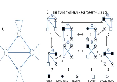
Theorem 6 implies restrictions on the possible sequences of set membership as we move through the target sequences from higher to lower value. Figure 1A shows the sequences which are not ruled out by Theorem 6. We can start at any vertex and proceed along the arrows. The number of possible paths of lengthnis (n+ 1)2, yielding an upper bound for the number of distinct set sequences. The
actual number of such sequences realised forn= 1−5 (obtained by computing the possibilities) is
{1,2,5,10,17}. Certain sequences are easy to exclude, for example we cannot have onlyb’s andd’s, orc’s andd’s. Forn= 4 we find additionally that sequencesbbba, bbaa, bbac, baac, bacc, aacc, accc
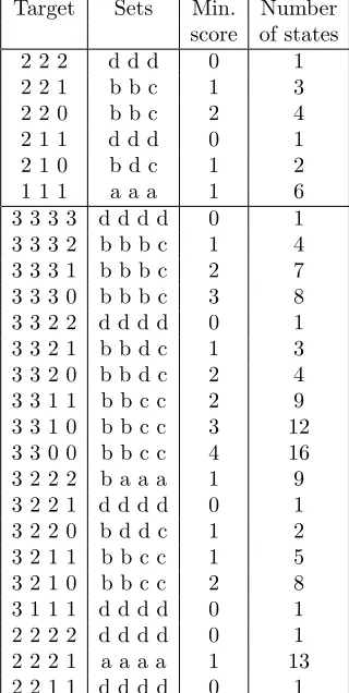
do not occur. Finally, we note that the number of ordered targets is2n−1Cn. Table 1 gives the set
membership of the vertices for the casesn= 3 andn= 4; the results for dual targets (as previously defined, if target t= (t1, t2, . . . , tn) then its dual is t∗ where t∗i = ((n−1)−ti)) can be deduced
straightforwardly. The number of states forK(min) is also given.
As stated before, a sequence with a score of 0 is graphic, and yields an end state where all individuals have payoff of zero. The next simplest case is a score of 1, where at every state of the minimum set there is a unique individual which has not achieved its target, and so has an incentive to change. This is one of the situations that we investigate in a subsequent paper. We note here that we have not considered mixed equilibria in the current paper at all, as this would require consideration of a new example and significantly lengthen the paper. That such equilibria exist will be demonstrated in the subsequent paper [8].
5. An illustrative game: the arithmetic case
In [6] we considered the following illustrative example, which is a member of the class of games that we termed “arithmetic” sequences, whereti=i−1 i= 1, . . . , n.
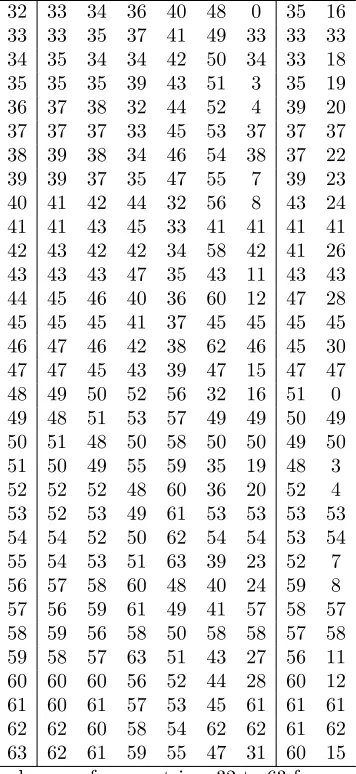
Example 5: the target {4,3,2,1,0}
The score for this target sequence is 2, yielding K(min) with eight elements. These are graphs, but we write them below in the form of their corresponding sequences, distinguishing between the two graphs that have the same sequence. We label them G1 toG8 in the following order 43221,
33220, 33211(1), 23210, 43212, 33211(2), 42211 and 32210 the state 33211(1) being the graph where the vertex with target 4 is joined to the vertex with target 0 (and thus the 3 is joined to the 1) while 33211(2) has the 4 joined to the 1 and the 3 joined to the 0. For the rest of this section, for simplicity we will simply denote the vertex with target i as ti (we note that the order from
a
b c
d
A
B
THE TRANSITION GRAPH FOR TARGET {4,3,2,1,0}
1 3 4 2
7 5 6 8
[image:16.612.137.538.109.393.2]JOINER DOUBLE JOINER NEUTRAL BREAKER DOUBLE BREAKER
Figure 1. 1A: Possible sequences of set membership. 1B: Schematic of the
transi-tion graph for the minimal graphs for target 43210. For each graph, the top symbol represents the vertex with target 2, which is always a neutral vertex. The vertices with targets 0,1,3,4 are represented by the symbols in the bottom left, bottom right, middle right and middle left positions, respectively. Each graph contains a specific set of links between the symbols, and the corresponding breaker or joiner status is given by the appropriate symbol. Possible transitions are shown by the arrows between the graphs.
Note that using Lemma 2, we can see that the target 3210 has the same set of solutions, by re-moving t2 and its edges from our original sequence. The score is, of course, again 2. If we order
the eight possible minimal graphs 3221, 2220, 2211(1), 1210, 3212, 2211(2), 3111, 2110, then the solutions are precisely the same as for the 43210 case. The transitions for target 43210 are shown in Figure 1B.
More generally for the arithmetic case with target sequence
t2m, t2m−1, . . . , tm+1, tm, tm−1, . . . , t2, t1, t0 we have that the subgraph of the m+ 1 vertices of
greatest degree is complete, and the subgraph of the m+ 1 vertices of lowest degree is empty. Thus we can replace the original target by two sequences with targets m, m−1, . . . ,2,1,0 and
m−1, m−2, . . .2,1,0 respectively, and restrict the acceptable graphs to bipartite graphs with the two sets corresponding to themof greatest degree and themof lowest degree in the original sequence. The central node, that is the originaltm with subsequent target 0 can be ignored. The
Target Sets Min. Number score of states 2 2 2 d d d 0 1 2 2 1 b b c 1 3 2 2 0 b b c 2 4 2 1 1 d d d 0 1 2 1 0 b d c 1 2 1 1 1 a a a 1 6 3 3 3 3 d d d d 0 1 3 3 3 2 b b b c 1 4 3 3 3 1 b b b c 2 7 3 3 3 0 b b b c 3 8 3 3 2 2 d d d d 0 1 3 3 2 1 b b d c 1 3 3 3 2 0 b b d c 2 4 3 3 1 1 b b c c 2 9 3 3 1 0 b b c c 3 12 3 3 0 0 b b c c 4 16 3 2 2 2 b a a a 1 9 3 2 2 1 d d d d 0 1 3 2 2 0 b d d c 1 2 3 2 1 1 b b c c 1 5 3 2 1 0 b b c c 2 8 3 1 1 1 d d d d 0 1 2 2 2 2 d d d d 0 1 2 2 2 1 a a a a 1 13 2 2 1 1 d d d d 0 1
Table 1. The set membership of vertices for targets with n= 3 and n= 4, and
number of graphs in the minimal set. The omitted sequences are all duals of those included.
Now at any point in time the system will be in some minimal graph. A vertex is picked at random with equal probabilities (i.e. 1/5), and that vertex might initiate a switch to another minimal graph, as per Figure 1B. For example suppose the current minimal graph isG1. Then if vertex
t4,t3ort2is picked no change can occur since they are currently at their target value, on the other
hand if vertext0is picked it must break its link witht4and so the minimal graph changes toG2,
while if vertext1 is picked it has a choice of breaking witht4, and thus the graph becomes G3, or
breaking witht3when the graph becomesG7. An individual’s strategy thus needs to specify which
of these to choose. We specify the transition probabilities for G1 as 3/5 to remain as 1, 1/5 to
switch to 2 andr1/5 the probability of choosingt4, ands1/5 the probability of choosing t3 where
r1+s1= 1.
There are six graphs where there are two different moves which stay within K(min). ForGi we
take probabilities ri and si when a choice is possible, that is when i = 1,2,4,5,7,8. We have
chosen the numbering of the minimal graphs so that Gi is obtained fromG9−i by reversing the
5∗A=
3 1 r1 0 0 0 s1 0
1 3 0 r2 0 0 0 s2
1 0 3 1 0 0 0 0 0 r4 s4 4 0 0 0 0
0 0 0 0 4 s5 r5 0
0 0 0 0 1 3 0 1
s7 0 0 0 r7 0 3 1
0 s8 0 0 0 r8 1 3
.
Note that had we chosen to work with the target 3210 the above matrix would have been modified by subtracting 1 from each diagonal element, and changing the scaling factor from 5 to 4, this affecting only the speed of convergence of the system, which would be quicker.
We consider only the case where each ri is either 0 or 1, i.e. pure strategies. Thus we have 64
possible transition matrices over the elements of K(min). In order to code the matrices we take the following functionf from the state number to a power of two (note that there are no choices to be made in states 3 and 6);f(1) = 1,f(2) = 2,f(4) = 4,f(5) = 8,f(7) = 16 andf(8) = 32. Then if the matrixA= (ai,j) hassi= 1 fori∈S⊆ {1,2,4,5,7,8} andsi= 0 otherwise, we take index
Σi∈Sf(i) for that matrix. There are symmetries which we can exploit. Thus if we haveA= (aij)
for someS andT ={i|(9−i)∈S}this gives matrix B= (bi,j) wherebi,j=an−i,n−j and so the
dominant eigenvector of B is the reverse of that of A. Equivalently if the binary expression for the index of Ais (i1i2i3i4i5i6) then (i6i5i4i3i2i1) is that ofB. We refer to matrix B as thedual
matrix ofA(not to be confused with the previously defined dual sequence), and the index ofBas
the dual of that ofA. Of course A is the dual ofB, as is A’s index the dual ofB’s. There are 8 matrices whereA=B, those with indices 0, 12, 18, 30, 33, 45, 51 and 63. Further discussion of the matrices and their eigenvectors is given in the Appendix.
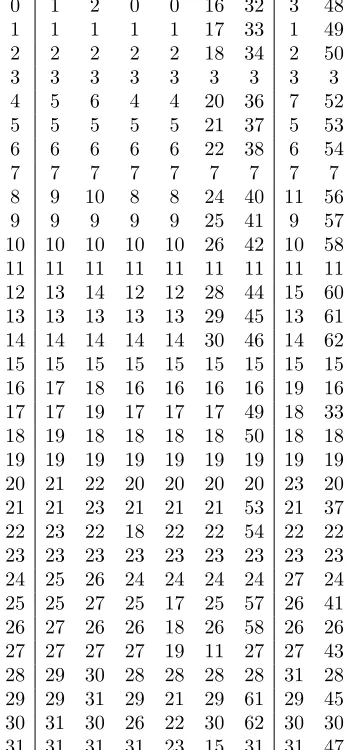
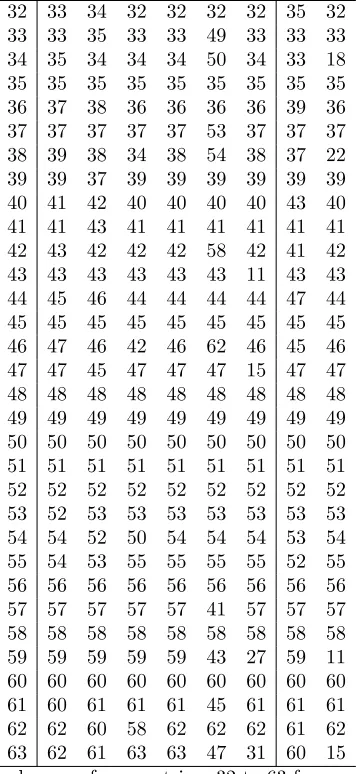
We label the matricesA0, A1, . . . , A63with connections as above. We suppose that when the current
set of strategies is specified byAithen the system will have converged to its stationary distribution,
which requires that strategic changes that lead to a change of matrix are infrequent in comparison to moves between graphs. The eigenvectors of the 64 matrices are given in Table 2 (see the Appendix). MatricesA0, A4, A8, A12have two unit eigenvalues, and thus have a two dimensional space for the
dominant eigenvectors. We denote the extreme eigenvectors of A0 by V0L = (0L,0,0,0,0) where
0L = (2,3,1,4) (see Table 2) and VR
0 = (0,0,0,0,0R) where 0R = (4,1,3,2). Similarly we have
8L = 0L, 4R= 0R, 8R= 12R= (4,3,1,2) and 4L= 12L= (2,1,3,4), and soV0L=V8L,V0R=V4R,
V8R =V12R and V4L =V12L. The matrices with indices 8,16,24,32,40,48,56 have eigenvector V0L, (note this is the set with sums of 0,8,16,32) while indices which are sums of 0,1,2,4 have eigenvector V0R, those with 8 plus sums of 0,1,2,4 have eigenvector V8R, and those with 4 plus
sums of 0,8,16,32 have eigenvectorVL
4 . The cases where the indices are 18,30,33,45,51,63 (where
A=B) have reversed eigenvectors, and when we haveA6=B the eigenvectors are the reverse of each other. Note that instead ofAi we simply writeiin much of what follows.
5.1. Payoffs and strategy switching. Given a stationary distributionπ= (π1, π2, . . . , π8), we
calculate the costci (which is minus the payoff) for each vertexti;c2= 0 since vertext2is always
neutral, and otherwise we have
c0=π1+π3+ 2π5+π6+π7,c1=π1+π2,c3=π7+π8,c4=π2+π3+ 2π4+π6+π8.
These costs are shown in Tables 3 and 4 (see the Appendix). Note that, with the exception of matrices 51, 55, 59 and 63, where all the costs are 0.5, the cost for one of vertices t0 and t4 is
always greater than 0.5, while the cost for verticest1andt3is always less than 0.5. The total cost
We consider the optimal strategies for the vertices. Suppose that the matrix has some current index from 0−63, the system currently has some particular graph from G1−G8 and a vertex
fromt0−t4is chosen at random. We consider its current payoff vis-a-vis those it would obtain by
making an allowable switch to a different strategy. Supposet0 is chosen then in graphsG2, G4, G8
the vertex is at its target, while in graphsG1, G3, G6, G7the vertex has a single link which it must
break. Accordingly no change will occur in the value of M. Vertex t0 only has a choice when
graph G5 occurs, so can switch from s5= 1 tos5= 0 or vice versa, i.e. decrease the index of the
current matrix by 8, or increase by 8, and then compare the current cost with that in the new matrix (at its new stationary distribution). In a similar manner vertext4will only have a choice if
the current graph isG4 when it can alters4so change state index by 4. For vertex 1 the situation
is somewhat different. There are two graphs where t1 has a choice, G1 andG2, which can cause
changes in the matrix index by 1 or 2 respectively. We may restrict the possible change to a single one, i.e. 1 or 2 (corresponding to local changes as defined in Section 3.3) or we may permit double changes in the index (corresponding to global changes). Similarly vertext3may change the index
by 16 or 32, or both. Thus for example if in matrix 5, fort0we can move to matrix 13, for vertex
t1 we can move to indices 4, 7 or if a double move permitted to 6, for vertex t3 to 21, 37 or with
a double move to 53 and for vertext4 to index 1. The possible choices and outcomes for matrix 5
are shown in Table 5 (see the Appendix).
We need to note that the possible invasions of states whose stationary distribution does not cover the whole space is restricted in some cases. For example suppose that the current matrix is 5. Then the possible neighbours (i.e. potential invaders) have indices 4,7,1,13,21,37 (the binary neighbours of 5 under a single change). The first three of these have the same stationary distribution as 5, the fourth has a different stationary distribution but with the same support, while the final two have stationary distributions with support the whole set. With a two-dimensional space for the dominant eigenvector we need to consider both extremes and then deduce the result for the whole space. For example if the state is 0 and the system is at the extreme 0L then switching to matrix indices 8, 16 or 32 will not change the stationary distribution. Switching to matrix 1 or 2 will cause a switch to a stationary distribution over the whole space. A switch to matrix 4 will cause a change but with the same restricted space, i.e. possibly to 4L. In general for VL there are 3 potential switches which leave the stationary distribution unchanged, one which changes the distribution but not the coverage, and two which would change to a distribution over the whole space. Whether a switch is made depends on the payoff to the vertex involved under the current matrix and that under the matrix resulting from a switch. We examine four scenarios, comprising either (1) switch only if the expected payoff increases or (2) switch if the expected payoff does not decrease, in combination with either (a) do not allow double switches or (b) allow double switches. The case where only an improvement allows a change might reflect that a cost is involved in the switch, albeit a small one. We refer to the four possibilities as 1a, 1b, 2a and 2b. We obtain radically different results, though we concentrate primarily on 1a. Later we consider the case where there is cost involved in switching.
As an example we suppose the current matrix index is 5. Table 5 gives the payoffs for the various vertices for matrix 5 and its various neighbours. The payoffs underlined are the ones that need to be compared, and those flanked with ∗’s are those payoffs which initiate a change under the various rules.
will be invasion by both 1 and 2. A similar argument implies that 3 will invade provided µ6= 0, while 16, 32 and 48 will invade providedµ6= 1. These arguments apply in all four cases, and in a similar way for the indices 4, 8 and 12. The remaining possible invasions by 4, and 8 are somewhat different. For case 1athere will be no invasion whereas in case 2a µ0L+ (1−µ)0Rwill be replaced
byµ4L+ (1−µ)4Randµ8L+ (1−µ)8R, respectively. Exceptional cases where for some state the
eigenvector is at the extreme of its two dimensional space are singular, i.e. only whenµis 0 or 1. In general we will not reach these odd states and so they can be omitted.
For both 1aand 1bit turns out that none of the 4 extreme matrices associated with indices 0, 4, 8 and 12 can invade any of the matrices outside of that set, and that each is invadable by other matrices. In each case there are 16 matrices which are absorbing (i.e. are pure Nash equilibria), (3; 48),(7; 56),(11; 52),(15; 60),(19; 50),(23; 58),(35; 49),45,51,
where those written together are the dual pairs. For 1a there are 18 states which could reach a PNE in one step, 21 which could reach a PNE in two steps and 9 which require at least three steps. The corresponding figures for 1bare 29, 15, and 4.
The first two pairs and 51 have no predecessors, i.e. there are no matrices from which our process will arrive at them. Additionally states 0,(4; 8),12,(55; 59),63 have no predecessors. For 1b we find essentially the same results, the set of eight above cannot invade outside their own set, and furthermore for the stable matrices the double change never allows an invasion.
For cases 1aand 1bthe transition matrix has no asymptotic cycles. The indexing we have intro-duced would allow for the representation of the matrices on the vertices of a 6-cube, the edges representing possible transitions. As an example of the possible flows we have illustrated the pos-sible transitions starting with matrices 4 and 8. None of the transitions when starting from matrix 4/8 involve a switch by 8/4. This allows the flow to be represented on a 5-cube, shown in Figure 2 2A.
In examining the possible changes which can be made for a given vertex we introduced the notion of a dual matrix. If the index of some matrixM is, in reversed binary notation, (i1i2i3i4i5i6) then we
refer toM∗with binary index (i6i5i4i3i2i1) as its dual; for exampleA27with binary index (110110)
has dual with binary index (011011) so matrix A∗27 = A54, and we write A∗27 = A54. Further if
we have a set of matricesT then we denote byT∗the set whose matrices are the duals of those inT. Now we have seen earlier that in 1avertext0only has a choice to exercise when the current graph
isG5, when a change alters the index by 8. We see from Tables 3 and 4 for which matrices there is
an improving change, and denote this set byT0,5 (a list of the matrices in the set is given below).
For vertext4when in graphG4a change alters the index by 4, with an improving change occurring
for the setT4,4=T0∗,5.
For verticest1andt3the situation is somewhat more complex. Fort1 there are two graphs where
a choice is available,G1 andG2. If the graph isG1 then vertext1 will have the option to change
the index by 1, while if G2 then a change by 2 is possible. Thus if t1 is chosen when the graph
is G1 then an improving change of the index by 1 will be made for the set of matrices denoted
byT1,1, 24 matrices in all. There are 16 pure Nash equilibria (PNEs) where obviously no change
would be made, and there are 24 other matrices where no change should be made. If vertext1 is
made to the matrices in setT1,2. Thus for vertext1 improvement will be made in matrices within
the setT1=T1,1TT1,2 irrespective of the graph.
Finally if vertex t3 is chosen when the graph isG7 then an improving change by index 16 should
be made for matrices in the set T3,7 =T1∗,2, and for vertex t3 in G8 improvements can be made,
changing the index by 32 in matrices T3,8 = T1∗,1. Changes at t3 should be from matrices from
the setT3=T1∗ irrespective of the graph. Note that for some matrices the stationary distribution
has zero probability for some graph. For example matrices 19,23,27,31,35,39,43,47,51,55,59,63 have zero probability forG4but these occur in pairs with the same payoff so there is not a change
in cases 1aor 1b.
T0,5={25,26,27,29,30,31}
T4,4={22,30,38,46,54,62}
T1,1={0,4,8,12,16,18,20,22,24,26,28,30,32,34,36,38,40,42,44,46,53,55,61,63}
T1,2={0,4,8,12,16,17,20,21,24,25,28,29,32,33,36,39,40,41,44,47,54,55,62,63}
T3,7={0,1,2,4,5,6,8,9,10,12,13,14,27,31,33,34,37,38,42,46,57,59,61,63}
T3,8={0,1,2,4,5,6,8,9,10,12,13,14,17,18,21,22,25,26,29,30,43,47,59,63}
T1={0,4,8,12,16,20,24,28,32,36,40,44,55,63}
T3={0,1,2,4,5,6,8,9,10,12,13,14,59,63}
The cases 2aand 2b are very different; there are no PNE’s, and both transition matrices over the 64 states are irreducible.
5.3. A switching fee. Suppose that there is a fee associated with switching. Thus if an individual has current costxand costy if it were to make a particular switch, then supposing there is a fee for switching ofzthe switch is only made ify+z < x. Thus cases 1a and 1b havez= 0+, while for
2a and 2b havez= 0. Table 10 (see the Appendix) gives the thresholds at which the set of PNEs increase. It is assumed that if a switch is made the new cost will apply for some large number of steps before a further switch is made. Thus a fee of z should be regarded as applying per time step. Figure 2B shows the possible flows, analogously to Figure 2A, when a cost of 0.1 is imposed. 5.4. Towards simpler rules. We have derived the changes which would lead to long term im-provement in the payoffs if the complex computation of the resulting stationary distribution were possible. In practice an individual at some vertex might only know its own links which for example would mean that individualt4would not be able to differentiate graphsG1,G5andG7, norG2,G6
andG8. It might know the links of all the vertices which would allow it to differentiate all the graph
states but again it would not know which matrix state applied. We discuss only the first of these cases. What information might be available to the individual? We might reasonably assume that it could keep track of the recent costs incurred, this providing an approximation to the cost incurred for this matrix. It might be able to keep track of the graphs through which it had most recently moved which would provide a proxy for the matrix. For example suppose that the system is cur-rently inG1and the most recent switches between graphs wereG8−> G2−> G4−> G2−> G1,
then under the assumption that during this period there were no changes of thesi, we can deduce
that s8 = 1, r2 = 1 and r4 = 1 so that the current matrix has 32 included in its binary index
etc. When an observation on the switch of each of graphsG1, G2, G4, G5, G7, G8 has been made
the matrix state can be determined. For example if the observed switches are respectively to
G7, G4, G1, G6, G1, G6 then one can infer that the matrix is 25. In similar manner provided that
over the period during which the information is collected there is no change of matrix, that matrix can be inferred exactly. If there is a switch of matrix then that might be immediately detected by an inconsistency in the recorded switches, and the collection of switches could be restarted. On the other hand it is possible that a switch of matrix might occur without causing an inconsistency, but since none of the earlier switches between graphs would be invalidated the individual can just update the appropriate data. In fact the individual just needs to keep track of the system until all of the six (potential) changes have been recorded.
Having obtained the matrix exactly then the correct switch, if any, would be determined from a check list for that vertex which might have evolved through time, though would require having a list of the 64 appropriate switches. Some simplification might be used. For example suppose we consider vertext0. Then we see from the 4th columns of Tables 6 and 7 (see the Appendix) that
a switch should be made only for the 6 matrices 25,26,27,29,30,31. These indices require 16 and 8, not 32, and at least one of 1 and 2. In a similar way for vertex t4 there are only six matrices
where a switch should be made 22,30,38,46,54,62 the analogues of those for vertext0, and the
matrices require 2 and 4, not 1, and at least one of 16 and 32. The situation for verticest1 andt3
is inevitably more complex.
5.5. A Threshold Model. We consider now a simple threshold model for decision-making by the individuals. Although it is unreasonable to expect the individuals to be able to compute the cost implications of making a specific change to their plays they will have a reasonable knowledge of their recent costs. Given that changes are likely to be infrequent, taking the average cost over the last few steps should approximate the true reward fairly well. Suppose then that given this good estimate any individual with a choice changes if this value is above some threshold. For simplicity suppose that individualst0 and t4 use the same thresholdh04 while individualst1 and
t3 useh13, a reasonable simplification sincet0andt4have the same distribution of costs, as dot1
andt3. Then a matrix will be stable if and only if max(c0, c4)< h04 andmax(c1, c3)< h13. For
example suppose we take thresholds h04 = 0.76 and t13 = 0.31, then{25,33,38} are the possible
stable matrices reached under this rule. Table 11 (see the Appendix) should be interpreted in the following way; for given thresholds everything to the left and below that threshold point is stable. We note that the entries which have no others below or to the left in the table are precisely those wherec0=c4and c1=c3. The other pairs of matrices have reversed costs e.g. c0 for 22 is equal
to c4 for 26. If the thresholds lie below the line joining (1.0,0.0) and (0.5,0.5) then none of the
matrices are stable. There is a switch at every matrix, and the system is irreducible.
The above presupposes that the thresholds are set at some point and are never changed. However this seems an unreasonable assumption. For example suppose that the thresholds were h04= 0.8
andh13 = 0.2 then the system will ultimately only be fixed at matrix 45. A change of threshold
h04to something less than 0.8 will make state 45 unstable, so that now all matrices are unstable.
5.6. A second threshold model. Suppose that each vertex can choose its immediate threshold i.e. h= (h0, h1, h3, h4). Now it is clear that the valuesh=cwherec= (c0, c1, c3, c4) occurs as in
Table 11 correspond to stable sets of matrices. Moreover sincec0+c1+c3+c4= 2 then theh/2’s
corresponding to these critical matrices lie in the 3-simplex. Now consider the spaceR4and define
forx≥(0,0,0,0) the set S(x+) ={z∈R4|z
i ≥xi, i= 1,4}. Now there are 31 distinct cost sets
all lying on the 3-simplex, we refer to these as critical points. Now for xandy definez=x∼y
byzi =max(xi, yi) i= 0,1,3,4. Then we have the set of critical points defined by “if x andy
4/8 5/40 20/10 21/42
22/26 23/58
6/24 7/56 18/18 19/50
38/25 39/57
34/17 35/49 54/27 55/59
52/11 53/43 50/19
36/9 37/41
1/32 2/16 4/8 16/2 32/1
C
4/8 5/40 20/10 21/42
22/26 23/58
6/24 7/56 18/18 19/50
38/25 39/57
34/17 35/49 54/27 55/59
52/11 53/43 50/19
36/9 37/41
1/32 2/16 4/8 16/2 32/1
[image:23.612.140.564.127.401.2]D
Figure 2. The transitions starting from matrices 4 and 8 on the 5-cube. The
indices of the vertices and of the edges have two numbers, corresponding to the matrix reached from matrix 4 and 8 respectively. For example matrices 22 can be reached from matrix 4 by 16 then 2 (see Table 6). From 22 one can reach 18, 23 and 54, and 22 can be reached from 6, 20 and 30. The possible transitions from 26 are 18, 23 and 58 and can be reached from 10, 24 and 30. Stable matrices are highlighted. 2A: cost=0, 2B: cost=0.1.
x andy thenSS
T is the set of critical points corresponding tox∼y, and the region in which these matrices are stable isS(x∼y)+.
For the cases 2a and 2b the system is much more complex. Tables 8 and 9 (see the Appendix) gives the possible moves. Note that if in the 1a/1b case, we have from Tables 6 and 7 that i is not invaded by some neighbourj, and j is not invaded by i, then the appropriate costs must be equal. Thus in Tables 8 and 9 we will have thatiandjcan invade each other. There are no stable matrices (PNEs) and it is easy to see that under 2a (and thus under 2b) the system is connected.
6. Discussion