Compressive techniques for sub-Nyquist data acquisition & processing in vibration-based structural health monitoring of engineering structures

(1)

City, University of London Institutional Repository

Citation: Gkoktsi, K. (2018). Compressive techniques for sub-Nyquist data acquisition &

processing in vibration-based structural health monitoring of engineering structures.

(Unpublished Doctoral thesis, City, University of London)

This is the accepted version of the paper.

This version of the publication may differ from the final published

version.

Permanent repository link: http://openaccess.city.ac.uk/19192/

Link to published version:

Copyright and reuse: City Research Online aims to make research

outputs of City, University of London available to a wider audience.

Copyright and Moral Rights remain with the author(s) and/or copyright

holders. URLs from City Research Online may be freely distributed and

linked to.

(2)

Compressive Techniques

for Sub-Nyquist Data Acquisition & Processing

in Vibration-based Structural Health Monitoring

of Engineering Structures

Thesis by

K

YRIAKI

G

KOKTSI

In partial fulfilment for the degree of

Doctor of Philosophy

C

ITY

,

U

NIVERSITY OF

L

ONDON

School of Mathematics, Computer Science & Engineering

Department of Civil Engineering

Research Centre for Civil Engineering Structures

(3)

(4)

C

ITY

,

U

NIVERSITY OF

L

ONDON

School of Mathematics,

Computer Science & Engineering

Department of Civil Engineering

Research Centre for Civil Engineering

Structures

Compressive Techniques for Sub-Nyquist Data

Acquisition & Processing in Vibration-based Structural

Health Monitoring of Engineering Structures

Doctoral Candidate: Kyriaki Gkoktsi

Supervisor: Dr Agathoklis Giaralis

Doctoral Committee: Dr

Stana Zivanovic

Dr Iasonas Triantis

(5)

(6)

Acknowledgements

First and foremost, I would like to thank my supervisor, Dr Agathoklis Giaralis for his mentorship, guidance, and continual support throughout my Ph.D studies. Over the last four years, Dr Giaralis has offered me unique opportunities that substantially contributed towards my academic and professional development, which I gratefully acknowledge. He has inspired me in various ways, and instilled great confidence in both myself and my research, being the most determining factors in making this work possible.

I am also particularly grateful to my research fellow, Dr Bamrung Tau Siesakul, for his valuable contribution in the initial stages of this research. He has introduced me to the electrical engineering discipline and helped me explore the world of signal processing. He has been a great colleague and friend, I cherish the days we were collaborating on a research project funded by EPSRC.

My sincere gratitude and appreciation is extended to Prof. Pol D. Spanos. It is difficult to express how honoured I feel for having been a visiting scholar in his research group. Prof. Spanos and his dedication to science have been an inspiration to me – thanks to him, I re-appreciated the beauty of maths. He has been a great mentor; his advice has always been invaluable to me.

I wish further to express my gratitude to Prof. Eleni Chatzi and to Dr Vasileios Dertimanis for our collaboration and for providing the field-recorded data used in Chapter 5 and Chapter 6 of this thesis. Special thanks are extended to my Ph.D committee members, Dr. Stana Zivanovic and Dr Iasonas Triantis for their insightful comments. My special gratitude goes to my supervisors on my diploma and MSc theses, Prof. ChristosIgnatakis and Prof. Kyriazis Pitilakis, for assisting and encouraging my decision to pursue a Ph.D at City, University of London.

I would like also to thank my friends and my family, especially my parents, for their unconditional love. Special thanks are extended to Angelina Damianou and Konstantinos Gkatzogias for their extremely valuable support and for being my closest companion over the last few years.

(11)

(12)

Declaration

(13)

(14)

Abstract

Vibration-based structural health monitoring (VSHM) is an automated method for assessing the integrity and performance of dynamically excited structures through processing of structural vibration response signals acquired by arrays of sensors. From a technological viewpoint, wireless sensor networks (WSNs) offer less obtrusive, more economical, and rapid VSHM deployments in civil structures compared to their tethered counterparts, especially in monitoring large-scale and geometrically complex structures. However, WSNs are constrained by certain practical issues related to local power supply at sensors and restrictions to the amount of wirelessly transmitted data due to increased power consumptions and bandwidth limitations in wireless communications.

The primary objective of this thesis is to resolve the above issues by considering sub-Nyquist data acquisition and processing techniques that involve simultaneous signal acquisition and compression before transmission. This drastically reduces the sampling and transmission requirements leading to reduced power consumptions up to 85-90% compared to conventional approaches at Nyquist rate. Within this context, the current state-of-the-art VSHM approaches exploits the theory of compressive sensing (CS) to acquire structural responses at non-uniform random sub-Nyquist sampling schemes. By exploiting the sparse structure of the analysed signals in a known vector basis (i.e., non-zero signal coefficients), the original time-domain signals are reconstructed at the uniform Nyquist grid by solving an underdetermined optimisation problem subject to signal sparsity constraints. However, the CS sparse recovery is a computationally intensive problem that strongly depends on and is limited by the sparsity attributes of the measured signals on a pre-defined expansion basis. This sparsity information, though, is unknown in real-time VSHM deployments while it is adversely affected by noisy environments encountered in practice.

(15)

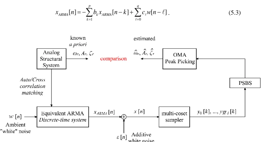
The second approach involves a novel signal-agnostic sub-Nyquist spectral estimation method free from sparsity constraints, which is proposed herein as a viable alternative for power-efficient WSNs in VSHM applications. The developed method relies on Power Spectrum Blind Sampling (PSBS) techniques together with a deterministic multi-coset sampling pattern, capable to acquire stationary structural responses at sub-Nyquist rates without imposing sparsity conditions. Based on a network of wireless sensors operating on the same sampling pattern, auto/cross power-spectral density estimates are computed directly from compressed data by solving an overdetermined optimisation problem; thus, by-passing the computationally intensive signal reconstruction operations in time-domain. This innovative approach can be fused with standard operational modal analysis algorithms to estimate the inherent resonant frequencies and modal deflected shapes of structures under low-amplitude ambient vibrations with the minimum power, computational and memory requirements at the sensor, while outperforming pertinent CS-based approaches. Based on the extracted modal information, numerous data-driven damage detection strategies can be further employed to evaluate the condition of the monitored structures.

(16)

List of Figures

Figure 1.1: Comparison of four different data acquisition schemes in wireless sensors for VSHM: (a) conventional; (b) CS-based; (c) PSBS-based; and (d) co-prime based approach…..5

Figure 2.1: Noiseless multi-tone signal in (a) time domain and (b) single-sided Fourier spectrum in frequency domain ……….……….13

Figure 2.2: Noisy multi-tone signal with SNR=0dB in (a) time domain and (b) single-sided

Fourier spectrum in frequency domain ………..………13

Figure 2.3: Compressive sensing measurement process with a random Gaussian measurement matrix Θ and the Inverse Discrete Fourier Transform IDFT matrix Ψ. The vector of coefficients u[n] is S-sparse (figure adapted from (Baraniuk 2007))…………...14

Figure 2.4: (a) Orthonormal IDFT basis Ψ N N , (b) selection of M random rows from Ψ 

 N N

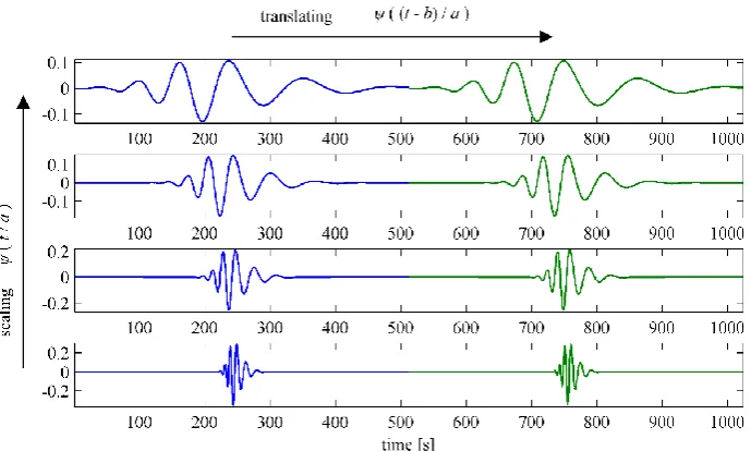
to derive (c) the partial IDFT matrix A M N ….………...16 Figure 3.1: Generation of a family of wavelet functions by scaling and translating in time the mother wavelet ψ(t) ………..28

Figure 3.2: Typical dyadic discrete wavelet transform (DWT) analysis filter bank with J=3 scales for processing N=8 long discrete-time signals ………..29

Figure 3.3: Daubechies D2 (or Haar) wavelets for four different scales j from a filter bank with J=16 total number of scales and Q= 0.49: (a) Normalised to the peak value Fourier Amplitude Spectrum, |Ψ(ω/2j)|; (b) wavelet in TD at scale j=11; and (c) wavelet in TD at scale j=14 ……….…..33

Figure 3.4: Daubechies D20 wavelets for four different scales j from a filter bank with J=16 total number of scales and Q= 0.46: (a) Normalised to the peak value Fourier Amplitude Spectrum, |Ψ(ω/2j)|; (b) wavelet in TD at scale j=11; and (c) wavelet in TD at scale j=14……….34

Figure 3.5: Meyer wavelets for four different scales j from a filter bank with J=16 total number of scales and Q= 0.68: (a) Normalised to the peak value Fourier Amplitude Spectrum, |Ψ(ω/2j)|; (b) wavelet in TD at scale j=11; and (c) wavelet in TD at scale j=14………35

Figure 3.6: Harmonic wavelets 10Hz constant bandwidth filter bank: (a) Fourier Amplitude Spectrum for 4 different scales with central frequencies denoted by broken lines, (b) real part harmonic wavelet with 15Hz central frequency, (c) real part harmonic wavelet with 35Hz central frequency………...37

Figure 3.7: Space truss FE models: (a) healthy state and (b) damaged state ……….…39

(17)

and (b) white noise excitation………..…41

Figure 3.10: Frequency domain representation of the normalised to unit amplitude response acceleration signals recorded at node 4 of the damaged space truss in Figure 7 under (a) sine-sweep and (b) white noise excitation……….……….41

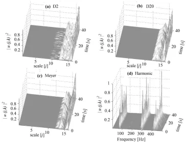
Figure 3.11: Normalised squared magnitude of wavelet coefficients pertaining to the truss acceleration response at node #4 (damaged state) under the sine-sweep excitation; discrete wavelet transform analysis with (a) D2 (Haar), (b) D20, (c) Meyer; and (d) Harmonic wavelet transform…..……….45

Figure 3.12: Normalised squared magnitude of wavelet coefficients pertaining to the truss acceleration response at node #4 (damaged state) under the white noise excitation; discrete wavelet transform analysis with (a) D2 (Haar), (b) D20, (c) Meyer; and (d) Harmonic wavelet transform ……….45

Figure 3.13: (a) Scale-dependent RWE(j) in eq. (3.18) and (b) RWE in eq. (3.10) using the Daubechies D2 (or Haar) wavelet filter bank for the space truss subject to the sine-sweep excitation ……….………48

Figure 3.14: (a) Scale-dependent RWE(j) in eq. (3.18) and (b) RWE in eq. (3.10) using the Daubechies D20 wavelet filter bank for the space truss subject to the sine-sweep excitation ………...……….48

Figure 3.15: (a) Scale-dependent RWE(j) in eq. (3.18) and (b) RWE in eq. (3.10) using the Meyer wavelet filter bank for the space truss subject to the sine-sweep excitation ………….48

Figure 3.16: (a) Scale-dependent RWE(j) in eq. (3.18) and (b) RWE in eq. (3.10) using a 128-scale harmonic wavelet filter bank (3.91Hz bandwidth per 128-scale) for the space truss subject to the sine-sweep excitation …..……….49

Figure 3.17: (a) Scale-dependent RWE(j) in eq. (3.18) and (b) RWE in eq. (3.10) using the Daubechies D2 (or Haar) wavelet filter bank for the space truss subject to the white noise excitation ………...………50

Figure 3.18: (a) Scale-dependent RWE(j) in eq. (3.18) and (b) RWE in eq. (3.10) using the Daubechies D20 wavelet filter bank for the space truss subject to the white noise excitation ………...……….50

Figure 3.19: (a) Scale-dependent RWE(j) in eq. (3.18) and (b) RWE in eq. (3.10) using the Meyer wavelet filter bank for the space truss subject to the white noise excitation ……….50

Figure 3.20: (a) Scale-dependent RWE(j) in eq. (3.18) and (b) RWE in eq. (3.10) using a 128-scale harmonic wavelet filter bank (3.91Hz bandwidth per 128-scale) for the space truss subject to the white noise excitation.………...……51

(18)

N=200 Nyquist samples; (a) sine-sweep excitation and (b) white noise excitation………...……..54

Figure 3.23: Normalised square magnitude of the reconstructed harmonic wavelet coefficients derived from the CR=30% compressed truss acceleration response (at node 4) for the (a) sine-sweep and (b) the white noise excitation……….55

Figure 3.24: (a) Scale-dependent CS-based RWE(j) in eq. (3.18) and (b) CS-based RWE in eq. (3.10) using reconstructed harmonic wavelet coefficients at CR=30% for the space truss subject to the sine-sweep excitation ………57

Figure 3.27: (a) Scale-dependent CS-based RWE(j) in eq. (3.18) and (b) CS-based RWE in eq. (3.10) using reconstructed harmonic wavelet coefficients at CR=30% for the space truss subject to the white noise excitation …...………58

Figure 3.28: (a) Scale-dependent CS-based RWE(j) in eq. (3.18) and (b) CS-based RWE in eq. (3.10) using reconstructed harmonic wavelet coefficients at CR=20% for the space truss subject to the white noise excitation …...………58

Figure 3.29: (a) Scale-dependent CS-based RWE(j) in eq. (3.18) and (b) CS-based RWE in eq. (3.10) using reconstructed harmonic wavelet coefficients at CR=10% for the space truss subject to the white noise excitation ..………58

Figure 4.1: Discrete-time model of the considered multi-coset sampling device proposed by Ariananda & Leus (2012)….………...65

Figure 4.2: Multi-coset sampling pattern with M̅ =3, N̅=8, K=4, and sampling sequence s=[0, 2, 5]T applied on a signal of 32 samples………...66

Figure 4.3: Workflow of the multi-sensor PSBS approach for OMA………...68

Figure 5.1: Adopted Monte Carlo simulation-based framework to assess the multi-coset sampling device for OMA applications ……….80

Figure 5.2: L-length simply supported beam with two degrees of freedom and the considered location of the excitation and measurement point at the 3L/8 and L/4 respectively….81

(19)

(blue curve) plotted against the target PSD in eq. (5.2) for the two adopted case studies: 2DOF with (a) well-separated and (b) closely-spaced modes of vibration……...……83

Figure 5.5: Considered frequency bands in the computation of the RMSE between recovered PSBS-PSD and target PSD for the 1st_{case study: (a) wide-band; (b) narrow-band}

around ω1; and (c) narrow-band around ω2……….……….84

Figure 5.6: Considered frequency bands in the computation of the RMSE between recovered PSBS-PSD and target PSD for the 2nd case study: (a) wide-band; (b) narrow-band around ω1; and (c) narrow-band around ω2……….……….84

Figure 5.7: RMSE versus observation’s window length, N, for the 1st case study with ω1=20rad/s

and ω2=60rad/s: (a) RMSE in the wide-band range of [0-100 rad/s]; (b) RMSE in the

narrow-band range of [10-30] rad/s (around ω1); (c) RMSE in the narrow-band range

of [50-60] rad/s (around ω2)………..………...86

Figure 5.8: RMSE versus CR for the 1st case study with ω1=20rad/s and ω2=60 rad/s: (a) RMSE

in the wide-band range of [0-100 rad/s]; (b) RMSE in the narrow-band range of [10-30] rad/s (around ω1); (c) RMSE in the narrow-band range of [50-60] rad/s (around

ω2)………..……….87

Figure 5.9: RMSE versus observation’s window length, N, for the 2nd case study with ω1=20rad/s and ω2=25rad/s: (left) RMSE in the wide-band range of [0-100 rad/s];

(middle) RMSE in the narrow-band range of [18.5-21.5] rad/s (around ω1); (right)

RMSE in the narrow-band range of [24-27] rad/s (around ω2) ………87

Figure 5.10: RMSE versus CR for the 2nd case study with ω1=20rad/s and ω2=25rad/s: (a) RMSE

in the wide-band range of [0-100 rad/s]; (b) RMSE in the narrow-band range of [18.5-21.5] rad/s (around ω1); (c) RMSE in the narrow-band range of [24-27] rad/s (around

ω2) ………..………..88

Figure 5.11: RMSE of the PSD estimates versus SNR for the two considered CRs in the 1st case study for (a) a wide frequency band, (b) a narrow band around ω1, and (c) around ω2;

N=39000 ……….………..89

Figure 5.12: RMSE of the PSD estimates versus SNR for the two considered CRs in the 2nd case study for (a) a wide frequency band, (b) a narrow band around ω1, and (c) around ω2;

N=39000 ……….………..89

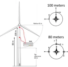
Figure 5.13: Wind turbine tower and location of sensors in the monitoring set-up (image reused from Chatzi & Spiridonakos (2015)) ………90

Figure 5.14: (a) Acceleration, (b) velocity, and (c) displacement time series acquired from sensor at 80m height (raw data)….……….90

Figure 5.15: Corrected/filtered (a) acceleration, (b) velocity, and (d) displacement time series (from sensor at 80m height) obtained from pre-processing the acceleration response in Figure 5.14………...91

(20)

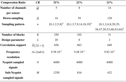
Figure 5.18: PSD estimates: Welch periodogram at Nyquist rate compared with PSBS approach for CR=11% (M̅ =14, N̅=128) in (a) logarithmic scale, and (b) linear scale……..……93

Figure 5.19: PSD estimates: Welch periodogram at Nyquist rate compared with PSBS approach for CR=21% (M̅ =8, N̅=39) in (a) logarithmic scale, and (b) linear scale …….………94

Figure 5.20: PSD estimates: Welch periodogram at Nyquist rate compared with PSBS approach for CR=31% (M̅ =5, N̅=16) in (a) logarithmic scale, and (b) linear scale ……….94

Figure 5.21: Considered space truss model………..96

Figure 5.22: Input/ output PSD estimates for the space truss in Figure 5.21; (a) input/white noise excitation signal; (b) output/acceleration responses measured at nodes #5 (blue curve) and #14 (red curve), respectively……….96

Figure 5.23: First singular values vector of the space truss response spectrum matrix in eq. (4.26) for CR={100%, 31%, 21%, 11%}……….…….99

Figure 5.24: Estimation of the 1st bending mode shape of the space truss; (a) conventional FDD at CR=100%; (b) PSBS-based FDD at CR=11%; and (c) MAC values versus CR….………100

Figure 5.25: Estimation of the 2nd bending mode shape of the space truss; (a) conventional FDD at CR=100%; (b) PSBS-based FDD at CR=11%; and (c) MAC values versus CR ………101

Figure 5.26: Estimation of the 3rd bending mode shape of the space truss; (a) conventional FDD at CR=100%; (b) PSBS-based FDD at CR=11%; and (c) MAC values versus CR ………101

Figure 5.27: Simply supported steel beam instrumented with 15 sampling devices measuring vertical acceleration response signals. ………..102

Figure 5.28: Damage states; DS0: intact/healthy structure; DS1: 50% stiffness reduction over 0.1m beam length; DS2: 50% stiffness reduction over 0.2m beam length; DS3: 80% stiffness reduction over 0.2m beam length ………103

Figure 5.29: PSBS-based FDD at CR=31% for mode shape estimation at DS0-DS3 for SNR=10dB (the horizontal axis gives the relative distance from the left support of the beam normalised with its length)………...105

Figure 5.30: Nyquist FDD versus PSBS-based FDD at CR=31% for mode shape estimation at DS0 for SNR=10dB (the horizontal axis gives the relative distance from the left support of the beam normalised with its length)………105

Figure 5.31: (a) Nyquist and (b) PSBS-based normalised modal strain energy index for DS0-DS3

and SNR=1020_{dB……….………..108}

(21)

Figure 6.1: Flowcharts of the two different sub-Nyquist sampling and spectral estimation approaches under comparison for frequency domain OMA………..113

Figure 6.2: Typical noisy acceleration response signal with SNR=10dB; (a) time history; (b): normalised single-sided Fourier spectrum magnitude; (c): Normalised magnitude Fourier coefficients in descending order. The red broken line signifies an arbitrary threshold at normalized Fourier magnitude of 0.05………...…………115

Figure 6.3: (a) Signal reconstruction error of CoSaMP algorithm versus the target sparsity level ST; (b-e) original and reconstructed DFT coefficients at CR={31%,11%}, ST={100,

290} for SNR=10 dB ………...118

Figure 6.4: PSBS spectral recovery and MSE for the low-sparse response accelerations (SNR=10 dB) at (a) CR=31% and (b) CR=11% …….………...118

Figure 6.5: Mode shape estimation for CR=31%, SNR=10dB (low-sparse signals) and target reconstruction sparsity ST=290 for the CS-based approach………..119

Figure 6.6: Mode shape estimation for CR=11%, SNR=10dB (low-sparse signals) and highest possible target reconstruction sparsity ST=290 in the CS-based approach………….119

Figure 6.7: MAC versus reconstruction sparsity level ST, obtained from the two considered

approaches, PSBS-based and CS-based FDD, for CR= 31%, SNR={1020,10}dB…120

approaches, PSBS-based and CS-based FDD, for CR= 11%, SNR={1020,10}dB….120

Figure 6.9: (a) Bärenbohlstrasse bridge in Zurich, Switzerland (image reused from Spiridonakos et al. (2016)) and (b) layout of the 18 sensors recording vertical acceleration responses under ambient excitation ……...………122

Figure 6.10: Typical acceleration-velocity-displacement time series recorded at sensor #13 pertaining to the raw data………...122

Figure 6.11: (a) Typical acceleration, (b) velocity, and (c) displacement time series recorded at sensor #13 pertaining to the corrected responses ……….……….123

Figure 6.12: (a) Normalised Fourier spectrum magnitude of the acceleration response signal measured at sensor #13, plotted within the frequency range of [0, 20] Hz; and (b) normalised magnitude Fourier coefficients sorted in descending order. The red broken line signifies an arbitrary threshold at normalized Fourier spectrum of 0.05……...123

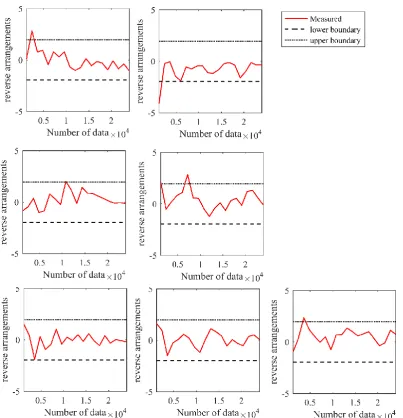
Figure 6.13: Reverse Arrangement method applied on acceleration response signal measured at sensor #13; signal is divided in 8 segments of 1min duration……….124

(22)

signal reconstruction of acceleration response signal at sensor #13 for ST=11160

(right)………127

Figure 6.16: (a) Compressive sensing at CR=21% and the acquisition of M=82 samples within a time-window of 2sec duration with N=400 Nyquist samples and (b) CoSaMP-based signal reconstruction of acceleration response signal at sensor #13 for

ST=7320……...………..127

Figure 6.17: (a) Compressive sensing at CR=11% and the acquisition of M=44 samples within a time-window of 2sec duration with N=400 Nyquist samples and (b) CoSaMP-based signal reconstruction of acceleration response signal at sensor #13 for

ST=3840……...………..127

Figure 6.18: First singular values vector of the bridge response spectrum matrix for CR={100%, 31% ,21%, 11%}………...128

Figure 6.19: Estimation of the 1st mode shape (bending) of the Bärenbohlstrasse bridge; (a) conventional/non-compressive FDD; (b) PSBS-based FDD at CR=11%; and (c) the CS-based approach for CR=11% and target reconstruction sparsity ST=3840 …..…130

Figure 6.20: Estimation of the 2nd mode shape (bending) of the Bärenbohlstrasse bridge; (a) conventional/non-compressive FDD; (b) PSBS-based FDD at CR=11%; and (c) the CS-based approach for CR=11% and target reconstruction sparsity

ST=3840………130

Figure 6.21: Estimation of the 3rd mode shape (rotational) of the Bärenbohlstrasse bridge; (a) conventional/non-compressive FDD; (b) PSBS-based FDD at CR=11%; and (c) the CS-based approach for CR=11% and target reconstruction sparsity

ST=3840………130

Figure 6.22: Estimation of the 4th mode shape (rotational) of the Bärenbohlstrasse bridge; (a) conventional/non-compressive FDD; (b) PSBS-based FDD at CR=11%; and (c) the CS-based approach for CR=11% and target reconstruction sparsity

ST=3840………131

approaches (i.e., PSBS-based and CS-based FDD) for CR= 31%...131

Figure 6.26: MAC with respect to CR; PSBS-based approach compared against CS-based

approach for ST=3600………...133

Figure 6.27: Estimates of the total energy requirements (left) and the battery life (right) with respect to CR for the bridge case study………..137

(23)

to (a) df/f=5% (f1=67Hz, f2=70Hz) and (b) df/f=6% (f1=66Hz, f2=70Hz)……..……148

Figure 7.2: Parametric analysis with respect to SNR for the MUSIC and co-prime method for df/f=5% (f1=67Hz, f2=70Hz); (a) N1=3, N2=7, resolution 23.81Hz (b) N1=5, N2=7,

resolution 14.29Hz (c) N1=7, N2=11, resolution 6.49Hz (b) N1=7, N2=13, resolution

5.49Hz………...151

Figure 7.3: Parametric analysis with respect to SNR for the MUSIC and co-prime method for df/f=6% (f1=66Hz, f2=70Hz); (a) N1=3, N2=7, resolution 23.81Hz (b) N1=5, N2=7,

resolution 14.29Hz (c) N1=7, N2=11, resolution 6.49Hz (b) N1=7, N2=13, resolution

5.49Hz………...152

Figure 7.4: Configuration details of the adopted reinforced concrete frame………...…153

Figure 7.5: Considered Chuetsu-oki (Japan, 2007) horizontal ground motion component: (a) Time-history, (b) Squared amplitude of Fourier spectrum……….153

Figure 7.6: Moment-curvature (M-φ) hysteretic curves at the left plastic hinge of the 1st storey beam for (a) damage state 1 and (b) damage state 2 ………...155

Figure 7.7: Spectrum estimation from noisy acceleration response signals with SNR=10dB at the (a) first, (b) second, and (c) third floor of the structure in Figure 7.4 (healthy state) subject to 80s duration white noise base excitation………158

Figure 7.8: MUSIC pseudo-spectra with co-prime sampling of noisy acceleration response signals with SNR=10dB at the (a) first, (b) second, and (c) third floor for the healthy and the damaged state 1 structure in Figure 7.4………...………...159

(24)

List of Tables

Table 3-1: Natural frequencies corresponding to in-plane vertical bending mode shapes for the space truss FE models………..39

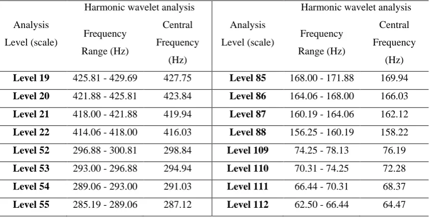
Table 3-2: Frequency domain attributes of the first 10 analysis levels for the considered wavelet filter banks………...43

Table 3-3: Frequency domain attributes of the non-constant Q harmonic wavelet transform for 16 analysis levels (in non-consecutive order) which include the first four resonant frequencies of truss in its healthy and damaged state………...………43

Table 5-1: Considered frequency ranges in the PSD estimates for the computation of the RMSE………..83

Table 5-2: Adopted multi-coset sampling values………...……..85

Table 5-3: Adopted ranges in parametric analyses………...……85

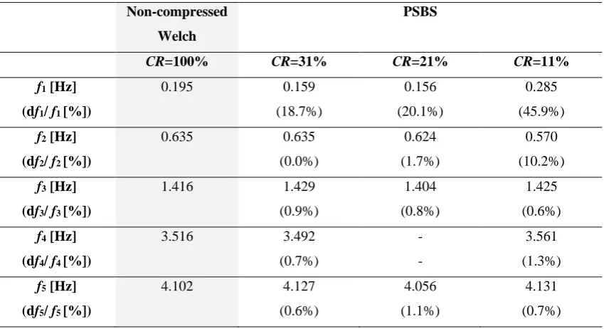
Table 5-4: Natural frequency estimates and percentage difference errors for the PSBS approach at CR={11%, 21%, 31%} and the standard welch modified periodogram applied on the full-length signal (non-compressed data with CR=100%)……….95

Table 5-5: Multi-coset pair (M̅ , N̅) and pattern sampling sequence………...………...98

Table 5-6: Natural Frequency Estimates ………..……...99

Table 5-7: Nyquist FDD versus PSBS-based FDD for natural frequency estimation at DS0-DS3

for SNR=1020dB………..…………..104

Table 5-8: Nyquist FDD versus PSBS-based FDD for natural frequency estimation at DS0-DS3 for SNR=10dB………..104

Table 5-9: Modal Assurance Criterion (PSBS-based FDD versus Nyquist FDD) on the estimated mode shapes at DS0-DS3 for SNR=1020 dB………..106

Table 5-10: Modal Assurance Criterion (PSBS-based FDD versus Nyquist FDD) on the estimated mode shapes at DS0-DS3 for SNR=10 dB……….106

Table 6-1: Considered parameters for the CS-based and the PSBS-based approaches for OMA of the structure in Figure 5.27 for two different compression ratios………...116

Table 6-2: Considered parameters for the CS-based and the PSBS-based approaches for OMA of the structure in Figure 6.9 for two different compression ratios……….125

Table 6-3: Natural Frequency Estimates from PSBS-based approach………129

(25)

Table 6-6: Daily energy consumption and remaining battery life for various CRs ………….136

Table 7-1: Adopted co-prime sampling values………...149

Table 7-2: Average secant flexural rigidity at yielding, ԐIy, at the ends of the frame structural

members of Figure 7.4………...154

Table 7-3: Flexural rigidity reduction factor (ԐIeff/ԐIy) at critical member zones of the structure in

Figure 7.4 for the two different damage states considered due to different seismic intensity excitation………155

Table 7-4: Assessment of MUSIC spectra from co-prime sampled noisy measurements for damage detection based on structural natural frequency shifts: damage state 1…….159

(26)

List of Symbols

ˆy

r

C covariance estimator matrix of output signal [ ]y k

Φ mode shape matrix

c

R pattern cross correlation matrix (R_c M2N) 2

x

 variance of input signal x[n]

O zero matrix

WMSE( )

f s cost-function of weighted mean square error criterion for the design of the multi- coset sampling pattern

( )

Λ α Diagonal matrix



Λ α( ) N N



(2L1)N

F Discrete Fourier Transform



2   



(2 2 1 1) 1 N L N

L N L

 

F

ˆ_{y y}a b

r estimated output cross-correlation matrix [ ]

i

c n filter coefficients of multi-coset sampling pattern ˆ_{x x}a b

r input cross-correlation estimate of signals x na

 

, x nb

 

[ ]

a b

x x

r k input cross-correlation function between the input signals x na

 

, x nb

 

a b x x

r

input cross-correlation matrix

(

_{x x}a b

)

N D



r

a b

x x

G input cross-power spectrum matrix of the input signals _{x n x n}a

   

, b

ˆ

a b x x

G input cross-spectrum estimate of signals x na

 

, x nb

 

1

N N

 

F

inverse discrete Fourier transform

WMSE

ˆ

s optimum design of the multi-coset sampling pattern, s

MMSE

ˆ

W optimum design of weighting matrix, W

, [ ] a b i j y y

r k _{output cross-correlation function of the compressed signals} a

 

i

y k , y kbj

 

a b

y y

r

_{output cross-correlation matrix} 2

( _{y y}a b ) M D 

r

[ ] i

(27)

( )

_n s scalar value associated with the multi-coset sampling pattern

,

ˆa b[ ]

i j

y y

r unbiased estimator of a_,b[ ]

i j

y y

r k

1/Ts Nyquist samplingrate (in Hz)

A CS partial measurement matrix of size MN, A=ΘΨ AJ+1-j “approximation” sequence of wavelet coefficients

Ar amplitude value related to mode shapes and modal participation factors

b time index/translational parameter in the wavelet transform Br sinusoidalamplitude

C constant within the CoSaMP algorithm

CR compression ratio

D number of sensors in a WSN (d=a=b=1,2,…,D) dbl diameter of the longitudinal reinforcement

DJ+1-j “detail” sequence of wavelet coefficients

E signal’s energy

e upper error bound in noisy CS reconstruction

e(f) signal’s vector

fmax highest frequency component in signal x(t)

fr natural frequency at the rth mode of vibration (in Hz)

Fs sampling frequency

fuk characteristic steel ultimate strength

fyk characteristic steel yielding strength

g[p] low-pass filter in multi-resolution analysis GMUSIC (f) pseudo-spectrum MUSIC estimator

Gq diagonal spectrum density matrix of the modal coordinates q(t)

Gx(ω) power spectrum of x(t)

h[p] high-pass filter in multi-resolution analysis

I identity matrix

j level of multi-resolution analysis – scale-related parameter of wavelet transform K number of blocks the reference signal is divided within the multi-coset sampling pattern

k translational-related parameter in the discrete wavelet transform L parameter related to correlation support

Lo shear span

Lpl plastic hinge length

(28)

M number of channels in multi-coset samplers (i, j =1,2,…,M) My bending moment at yielding

M-φ Moment-curvature pair

N̅ down-sampling parameter in multi-coset samplers

N̅ number of uniform samples in each K block in the multi-coset sampling pattern N length of original/reference/uncompressed signal

N1,N2 co-prime numbers

NR number of realizations

Q ratio of effective frequency over the effective bandwidth at each analysis level

q(t) modal coordinate matrix

qr(t) modal coordinates at the r-th mode of vibration

R number of structural modes of vibration (r



1, 2,,R



)

Rss spatially-smoothed correlation matrix

ry correlation matrix

Ryy auto-correlation function of y[k]

s sequence of multi-coset sampling pattern

S signal sparsity

si, sj coset/ delay parameter at the m-th channel of the multi-coset sampler

ST target sparsity in reconstructed time-domain signals

SWE Shannon wavelet entropy

Ts sampling rate

U unitary singular matrices holding the left singular vectors u(α,b) wavelet coefficients

u[n] discrete Fourier transform coefficients

û[n] recovered signal coefficients on the DFT domain

V unitary singular matrices holding the right singular vectors v(u) auxiliary smoothing function in Meyer wavelet functions

W weighting matrix

wj energy ratio at scale j for a potentially damaged structure

x(t) real-valued signal in time domain

X(ω) Fourier transform of signal x(t) in frequency domain x[n] input full-length discrete-time signal

(29)

α scaling parameter in wavelet transform δS restricted isometry constant

ε measurement error vector

ε[k] zero-mean complex Gaussian white noise sequences; noise sequence component η tolerance parameter in CoSaMP algorithm

Θ measurement matrix in compressive sensingof size MN

θr random phase

μφ curvature ductility

Σ diagonal positive semi-definite matrix comprising the singular values, Σrr, at the

r-th mode of vibration σ2 _{variance, signal’s power}

Το total length (duration) of the time interval

φ structural mode shapes/eigenvectors φ(t) scaling function in wavelet transform

φr structural mode shapes/eigenvectors at the r-th mode of vibration

φy curvature at yielding

Ψ Basis matrix of size NN ψ(t) wavelet function

ω circular frequency (in rad/s)

Ω set of numbers

ωc central or the dominant frequency of the (unscaled) mother wavelet

ωeff effective frequency of wavelet function

(30)

List of Operations

p

 p norm

 absolute value

 discrete-time convolution operator

x complex conjugate of x

,

n m

 Dirac delta function

ˆ

x estimated value of x

a

E {} expectation operator with respect to a



  floor operator

 

H

 Hermitian transpose

 Imaginary part of complex number

 Kronecker product operator

 

1

 matrix inverse

 

_ T

matrix transpose

 

vec



matrix vectorisation

 

†

 Moore-Penrose pseudo-inverse

(31)

(32)

Glossary of Acronyms

ADC Analog-to-Digital Converter ARMA Auto-Regressive Moving Average

CoSaMP Compressive Sampling Matching Pursuit; signal recovery algorithm

CR Compression ratio

CS Compressive Sensing

DFT Discrete Fourier Transform

DP Daubechies wavelet of an P-length finite impulse response

DS Damage State

FDD Frequency Domain Decomposition

FE Finite Element

FFT Fast Fourier Transform FRF Frequency Response Function IDFT Inverse Discrete Fourier Transform MAC Modal Assurance Criterion

MSE Mean Square Error

MSEI Modal Strain Energy Index MUSIC Multiple Signal Classification OMA Operational Modal Analysis PGA Peak Ground Acceleration PSBS Power Spectrum Blind Sampling PSD Power Spectrum Density RMSE Root Mean Square Error RWE Relative Wavelet Entropy SHM Structural Health Monitoring SNR Signal-to-Noise Ratio

SVD Singular Value Decomposition

VSHM Vibration-based Structural Health Monitoring WMSE Weighted Mean Square Error

(33)

(34)

Chapter 1 Introduction

1.1. Structural Health Monitoring

Structural Health Monitoring (SHM) of civil engineering structures such as buildings, bridges, dams, masts, etc., aims to assess their structural integrity and performance either periodically or following extreme events/actions (i.e., floods, earthquakes, structural upgrades, blast loading) (e.g., Brownjohn (2007)). Periodic structural assessment is pursued by long term SHM seeking to capture the gradual structural changes due to operational and environmental conditions (aging, degradation, thermal loading, etc.) and to provide useful information for structural maintenance and retrofitting, as well as validation of design models (e.g., Brownjohn (2007)). In the occurrence of extreme events, short term SHM involves rapid and real-time monitoring to provide information for intermediate structural integrity. Ideally, SHM should extract the maximum information at minimum time without interrupting the structure’s normal functionality.

For most of the existing structures, apart from visual inspections which tend to be qualitative and non-continuous, vibration-based SHM (VSHM) is arguably the most commonly used method for global condition assessment (e.g., Lynch & Loh (2006); Lynch (2007); Nagayama & Spencer (2007); Spencer & Yun (2010)). It relies on acquisition and processing of structural dynamic response signals (e.g., acceleration responses) measured by sensors placed on structures exposed to time-varying loads, for the purpose of (i) estimating the inherent dynamic/modal properties of linearly vibrating structures under operational conditions, and (ii) detecting potential structural damage from vibration measurements.

The first purpose above concerns the so-called modal identification problem, which is divided into experimentalandoperationalmodal analysis depending on the type of the excitation force, i.e., measured-deterministic signals or unmeasured-stochastic processes, respectively (e.g., Reynders (2012)). Traditional Experimental Modal Analysis (EMA) measures both input (excitation) and output (response) signals to infer structural vibration characteristics (i.e., natural frequencies ωr, damping ratio ζr, mode shapes φr). It is mainly applicable to laboratory

(35)

On the antipode, Operational Modal Analysis (OMA) – also known as ambient, natural excitation or output-only modal analysis– utilises unmeasured ambient/natural excitation forces (e.g., wind, vehicle, and pedestrian traffic), assumed to be wide-sense stationary stochastic processes observing a sufficiently flat spectrum across a wide frequency band that can be approximated as Gaussian white noise (i.e., stochastic quantities with unknown parameters but with known behaviour) (e.g., Zhang et al. (2005); Reynders (2012)). OMA is suitable for real-time monitoring of large-scale and complex structures with the minimum cost and network disruption, being particularly useful in cases where it is difficult or unaffordable to measure the input forces, and/or when controllable excitation of structures is not possible in practice (e.g., Amezquita-Sanchez & Adeli (2016)). However, OMA may encounter bias errors, measurement noise, and other un-modelled effects and thus validation criteria are employed to assess the quality of the extracted modal estimates (e.g., Zhang et al. (2005)).

Moving next to the structural damage detection problem in the VSHM framework, four different aims are normally set, i.e., (1) identification of the existence of structural damage; (2) detection of its location; (3) damage classification, and (4) quantification of damage severity in terms of structural serviceability/durability (e.g., Ewins (2000); Humar et al. (2006)). A plethora of damage detection algorithms have been proposed, capable to derive damage-sensitive indices by processing dynamic response signals, measured between the current (potentially damaged) and a past baseline (“healthy”) structural state (e.g., Sohn & Farrar (2001); Worden et al. (2007)).

(36)

1.2. Conventional Wireless Sensor Networks (WSN) in VSHM

Over the last two decades, the consideration of wireless sensor networks (WSNs) has been an important development in VSHM of civil structures (e.g., Lynch & Loh (2006); Lynch (2007); Nagayama & Spencer (2007); Spencer & Yun (2010)). It has emerged as a viable alternative to cabled sensor networks which are restricted by costly and labour-intensive installations of long coaxial wires. Specifically, WSNs enable dense structural instrumentation and access to remote locations on structures, offering less obtrusive, rapid, and more economical VSHM implementations, especially in monitoring large-scale and geometrically complex civil engineering structures. Compared to arrays of wired sensors, the reduction in cost is reported to be one to two orders of magnitude per sensing channel in real life applications (e.g., Spencer & Yun (2010)). Thus, WSNs are particularly suited for periodic VSHM of the large stocks of existing structures and for VSHM in the aftermath of natural disasters in densely populated areas.

Nonetheless, wireless sensors are mainly powered by batteries in need of frequent replacement (e.g., from few weeks to few months depending on the application and the sampling considerations). Apart from the environmental impact, this has a direct impact on the maintenance cost of “permanent” VSHM in large-scale deployments and poses constraints to the rapid assessment of large number of structures. Alternatively, energy harvesting solutions can be used to power WSNs by exploiting environmental energy sources (e.g., wind, solar, thermal, etc.) – however, such solutions increase the overall cost for sensor deployment and pose restrictions in sensors placement. Thus, the consensus is that WSNs will become the preferred way for low-cost VSHM in civil structures once its major limitation – energy supply and power consumption – is addressed in a cost-effective manner (e.g., Lynch & Loh (2006); Lynch (2007)).

A typical WSN used for VSHM is composed of wireless sensors – equipped with a sensing interface, computational core, and wireless transceiver – and a server (base station) that collects the transmitted measurements for further processing. In each component, the following operations are performed (see also Figure 1.1(a) and Lynch & Loh (2006); Lynch (2007); Nagayama & Spencer (2007); Novakovic et al. (2009); Spencer & Yun (2010)):

• Sensing interface (wireless sensor): Traditional analog-to-digital converters (ADCs) are utilised to acquire structural responses at the uniform Nyquist rate, which is defined as twice the highest frequency component in the measured signals (i.e., twice the signal’s bandwidth, e.g., Jerri (1977)). In practical applications, though, faster sampling rates are employed followed by low-pass filtering to eliminate any potential aliasing and to increase resolution.

(37)

lossy or lossless data compression (e.g., Duarte et al. (2012)). The main goal of this operation is to address the increased power demands and bandwidth limitations in wireless transceivers.

• Wireless Transceiver(wireless sensor): This building block is responsible for the wireless communication between sensors and server by wirelessly transmitting and receiving the measured data. Notably, wireless data transmission is by far the most power consuming operation in WSNs ((e.g., Lynch (2007)), being inextricably linked with the local energy harvesting and/or battery replacement requirements in wireless sensors. The wireless transceivers are also constrained by the limited available wireless transmission bandwidth, posing limitations on the amount of data that can be reliably transmitted within WSNs. • Server (base station): After wireless data transmission to the server, the encoded

measurements (i.e., compressed data) are de-compressed to retrieve the originally acquired signals, or an estimate of them in case of lossy compression schemes. The recovered measurements can be further processed by standard VSHM algorithms to retrieve the salient features of the monitored structures.

Despite these efforts, the power resources of current WSNs are limited by the technical specifications of conventional wireless sensors, associated with the power consumption in the above operations (i.e., sampling and analog-to-digital conversion; computational and memory requirements; wireless communications among sensors and server, e.g., Lynch & Loh (2006); Lynch (2007); Nagayama & Spencer (2007); Novakovic et al. (2009); Spencer & Yun (2010)). Within this context, the most important factors are:

• the sampling considerations, i.e., the sampling rate and resolution, continuous or periodic sampling and the pertinent duration of each monitoring interval, the length of the acquired dataset and the number of transmitted data;

• the computational efficiency, i.e., the on-board hardware and software to be executed; • the network size, i.e.,the number of wireless sensors within the network;

• the network topology and the wireless communication protocol, controlling the power consumption by minimising the wireless transmission range and increasing the communication reliability by addressing the problem of information loss (i.e., due to missing data packets and/or multipath fading when radio waves are masked by obstacles, etc.);

(38)

• other issues related to errors due to inherent measurement noise in sensors, as well as spatial issues associated with the positioning of sensors.

Figure 1.1: Comparison of four different data acquisition schemes in wireless sensors for VSHM:

(a) conventional; (b) CS-based; (c) PSBS-based; and (d) co-prime based approach

1.3. Sub-Nyquist Data Acquisition Schemes for Low-Power WSNs in

VSHM

Recent advances in sub-Nyquist sampling schemes have paved the way for the development of Analog-to-Information Converters that involve simultaneous signal acquisition and compression at the sensor front-end prior to wireless transmission (e.g., Tropp et al. (2006), (2010); Bajwa et al. (2007); Mishali & Eldar (2010); Baraniuk et al. (2011); Jingchao et al. (2015); Moon et al. (2015)). Arguably, this technological breakthrough can offer viable alternatives for low-power WSNs in VSHM deployments, leading to significant savings in wireless communications (e.g., O’Connor et al. (2014)). The latter is accomplished by considering low-rate non-uniform sampling strategies (below the Nyquist rate) capable to:

• Reduce the sampling and power requirements in the sensing interface;

• Minimise the dimensions of transmitted data, yielding drastic reductions in the consumed power during wireless communications while efficiently addressing the pertinent bandwidth limitations;

• By-pass the computational requirements for on-sensor data storage and local on-board data processing before wireless transmission; and

(39)

Motivated by the above advances, this thesis focuses on the development of novel algorithmic

approaches based on compressive/sub-Nyquist data acquisition and processing techniques to

address the power constraints in WSNs used for operational modal analysis and data-driven

damage detection in civil engineering structures.

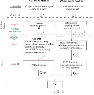
This line of research has been primarily triggered by developments in the field of Compressive Sensing (CS) (e.g., Candès et al. (2006); Donoho (2006); Baraniuk (2007)) – a recently proposed sub-Nyquist sampling scheme that exploits the signal’s sparsity (i.e., the non-zero signal coefficients) on an orthonormal basis to achieve dimensionality reduction. Based on random non-uniform in time data acquisition techniques at average sampling rates below Nyquist, Candès proved that any sparse signal can be reconstructed, with high probability, at the uniform Nyquist grid from a relatively small number of random measurements by solving an underdetermined system of linear equations subject to sparsity constraints (e.g., Candès (2008)).

Interestingly, the CS theory is valid within the VSHM framework since structural vibration responses preserve a compressible (i.e., nearly sparse) structure in various domains and co-domains (e.g., noiseless response acceleration signals from linear vibrating structures tend to be appreciably sparse in the frequency domain, since their Fourier coefficients with non-negligible magnitudes are clustered around their natural frequencies). These important findings have motivated numerous VSHM research studies in the literature over the last decade, aiming to provide quality structural estimates from compressed data while efficiently addressing the WSN challenges related to bandwidth constraints, limited power resources, and loss of information due to wireless data transmissions. In this respect, O’Connor et al. (2014) developed the CS-based approach shown in Figure 1.1 (b), which was implemented in the first long-term VSHM field deployment using customised Analog-to-Information Converters. Given its successful implementation, the approach of O’Connor et al. is treated herein as a paradigm of CS-based VSHM using low-rate randomly sampled measurements; thus, it is adopted in this study for comparative purposes. Nonetheless, the CS sparse recovery is a computationally intensive problem that strongly depends on the sparsity attributes of the measured signals on a pre-defined

vector basis. This sparsity information, though, is unknown in real-time VSHM deployments while

it is adversely affected by noisy environments encountered in practice (e.g., Bao et al. (2011); O’Connor et al. (2014); Huang et al. (2016)).

1.4. Aims and Objectives

(40)

detection algorithm is developed herein, capable to retrieve data-driven damage indices directly from compressive data without reconstructing structural responses in time-domain. The proposed method couples the CS framework with the Relative Wavelet Entropy (RWE), a well-established in the literature damage-sensitive index (e.g., Ren & Sun (2008); Yun et al. (2011); Lee et al. (2014)) derived by wavelet transforming response acceleration signals obtained from a healthy/reference and a damaged state of a given (linear) structure subject to broadband excitations.

The second goal is to develop a novel signal-agnostic sub-Nyquist spectral estimation strategy (Figure 1.1 (c)) free from sparsity constraints, which is proposed herein as a viable alternative for power-efficient WSNs in VSHM applications. The developed strategy relies on Power Spectrum Blind Sampling (PSBS) techniques (see also Leus & Ariananda (2011)) together with a deterministic non-uniform-in-time sampling scheme, known as multi-coset sampling (e.g.., Venkataramani & Bresler (2001)), which can be implemented by utilising M interleaved ADCs each operating N times slower than the Nyquist rate



M N



. Ultimately, this novel approach in Figure 1.1 (c) can retrieve auto/cross power spectral estimates of non-sparse wide-sense stationary random signals (i.e., stochastic processes) directly from compressed measurements, by-passing the computationally demanding signal reconstruction operations in time-domain. This is achieved based on a weighted least-squares optimisation criterion (e.g., Tausiesakul & Gonzalez-Prelcic (2013)) which mathematically defines an overdetermined system of linear equations that can be easily solved.

(41)

significantly reduced number of measurements with super-high resolution while filtering out additive broadband noise.

1.5. List of Referred Papers

Parts of this thesis, indicated in the next sub-sections, have already been published, or submitted for publication, in the following peer-reviewed journal papers and conference proceedings.

1.5.1. Journal papers

[J1] Gkoktsi, K. & Giaralis, A., 2015. Effect of frequency domain attributes of wavelet analysis filter banks for structural damage localization using the relative wavelet entropy index. International Journal of Sustainable Materials and Structural Systems (IJSMSS), 2(1/2), pp.134–160.

[J2] Gkoktsi, K. & Giaralis, A., 2017. Assessment of sub-Nyquist deterministic and random data sampling techniques for operational modal analysis. Structural Health Monitoring: An International Journal, 16(5), pp.630–646.

[J3] Gkoktsi, K. & Giaralis, A., 2018. A multi-sensor sub-Nyquist power spectrum blind sampling approach for low-power wireless sensors in operational modal analysis applications. Mech. Syst. Signal Process. (under review, submitted September 2017).

1.5.2. Conference proceedings

[C1] Gkoktsi, K. & Giaralis, A., 2014. On the influence of frequency selectivity of wavelet bases for relative wavelet entropy-based structural damage localization. In 6th World Conference on Structural Control and Monitoring (6WCSCM). pp. 1366–1378.

[C2] Tausiesakul, B., Gkoktsi, K. & Giaralis, A., 2014. Compressive Sensing Spectral Estimation For Output-Only Structural System Identidication. In 7th International Conference on Computational Stochastic Mechanics. pp. 1–12.

[C3] TauSiesakul, B., Gkoktsi, K. & Giaralis, A., 2015. Compressive power spectrum sensing for vibration-based output-only system identification of structural systems in the presence of noise. In SPIE Sensing Technology + Applications.

[C4] Gkoktsi, K., TauSiesakul, B. & Giaralis, A., 2015. Multi-channel sub-Nyquist cross-Spectral Estimation for Modal Analysis of Vibrating Structures. In International Conference on Systems, Signals and Image Processing (IWSSIP 2015).

[C5] Gkoktsi, K., Giaralis, A. & TauSiesakul, B., 2016. Sub-Nyquist signal-reconstruction-free operational modal analysis and damage detection in the presence of noise. In J. P. Lynch, ed. SPIE Smart Structures and Materials + Nondestructive Evaluation and Health Monitoring. International Society for Optics and Photonics, p. 980312.

[C6] Gkoktsi, K. & Giaralis, A., 2016. Assessment of sub-Nyquist deterministic and random data sampling techniques for operational modal analysis. In 8th European Workshop On Structural Health Monitoring (EWSHM 2016). Bilbao, Spain.

(42)

[C8] Gkoktsi, K., Giaralis, A. & Tausiesakul, B., 2017. A reconstruction-free sub-Nyquist sensing approach for earthquake damage detection using the MUSIC algorithm. In 16th World Conference on Earthquake Engineering.

1.6. Thesis Organisation

This thesis is divided into eight chapters. The current introductory chapter (§1. Introduction) gives a general overview of the notion of the vibration-based structural health monitoring (VSHM) in civil engineering structures using wireless sensor networks (WSN) and reports the limitations encountered in conventional and advanced approaches, concluding with the scope of this thesis and the aims and objectives set. Chapter 2 (§2.Compressive Sensing: Basic Concepts & Applications in VSHM) presents the basic principles of the Compressive Sensing (CS) theory and reviews the state-of-the-art in CS-based VSHM approaches for civil structures, underlying the main factors that limit their performance. Recognising that CS is constrained by signal sparsity requirements on a pre-defined vector basis, a comprehensive numerical study is undertaken in Chapter 3 (§3. CS-based Damage Detection Using the Relative Wavelet Entropy) to define the “sparsest” representation of structural responses on the wavelet transform domain using various wavelet analysis filter banks with different frequency domain attributes. From these findings, a novel CS-based RWE damage detection algorithm is further proposed for data-driven VSHM deployments using dense arrays of wireless sensors with reduced power demands. (Parts of Chapter 3 have been published in the journal paper [J1] of §1.5.1, and in the conference

proceedings [C1] of §1.5.2).

Compressive techniques for sub-Nyquist data acquisition & processing in vibration-based structural health monitoring of engineering structures

City, University of London Institutional Repository

Citation: Gkoktsi, K. (2018). Compressive techniques for sub-Nyquist data acquisition &

This is the accepted version of the paper.

This version of the publication may differ from the final published

version.

Permanent repository link: http://openaccess.city.ac.uk/19192/

Link to published version:

Copyright and reuse: City Research Online aims to make research

outputs of City, University of London available to a wider audience.

Copyright and Moral Rights remain with the author(s) and/or copyright

holders. URLs from City Research Online may be freely distributed and

linked to.

Compressive Techniques

for Sub-Nyquist Data Acquisition & Processing

in Vibration-based Structural Health Monitoring

of Engineering Structures

Thesis by

K

YRIAKI

G

KOKTSI

In partial fulfilment for the degree of

Doctor of Philosophy

C

ITY

,

U

NIVERSITY OF

L

ONDON

School of Mathematics, Computer Science & Engineering

Department of Civil Engineering

Research Centre for Civil Engineering Structures

C

,

U

L

School of Mathematics,

Computer Science & Engineering

Department of Civil Engineering

Research Centre for Civil Engineering

Structures

Compressive Techniques for Sub-Nyquist Data

Acquisition & Processing in Vibration-based Structural

Health Monitoring of Engineering Structures

Doctoral Candidate: Kyriaki Gkoktsi

Supervisor: Dr Agathoklis Giaralis

Doctoral Committee: Dr

Stana Zivanovic

Dr Iasonas Triantis

Contents

Acknowledgements

Declaration

Abstract

List of Figures

List of Tables

List of Symbols









 

 

 

 

r

(

)



r

   

 

 

F

 

 

r



