Standardisation of wind turbine SCADA data for gearbox fault detection

Standardisation of Wind Turbine SCADA Data for Gearbox Fault

Detection

D Ferguson*, A McDonald*, J Carroll*, H. Lee

*University of Strathclyde, Scotland, [email protected], •Offshore Renewable Energy Catapult, Blyth, UK

Keywords: Anomaly detection, gearbox, standardisation, monitoring.

Abstract

This paper presents a method of anomaly detection within a gearbox by way of standardising temperature data. Assessing measured parameters in isolation is not sufficient to detect faults within a wind turbine. This technique uses temperature, rotational speed and generator torque to detect a bearing fault within the gearbox. Standardising data allows a parameter to be analysed which also takes into consideration the operating state of the wind turbine, therefore providing a more holistic view of the health of the wind turbine and component being monitored.

1 Introduction

Wind power is now the second largest energy producer in Europe with an installed capacity of 169GW [1]. Although the cost of energy from wind power has fallen significantly in recent year’s operations and maintenance costs still account for a significant proportion (around 30% [2]) of the costs, especially for offshore wind farms. Condition monitoring systems are now beginning to play a major role in reducing the operations and maintenance costs by allowing better scheduling of maintenance and the avoidance of major component failures. Of these major component failures it is the generator and gearbox which account for the largest loss of production due to the downtime resulting from a failure [3].

The work presented here focuses on the detection of faults within the wind turbine gearbox. Unlike conventional power generation methods, detecting faults within a wind turbine gearbox is more challenging due to varying frequencies that result from the continuously changing wind speed. The varying wind speed means that the load on the generator and gearbox is continuously changing in order to allow for maximum energy capture. The ever changing operating state coupled with the changing ambient weather conditions means that a holistic view must be taken when monitoring the health of a wind turbine.

There are a number of techniques in literature which take into account the need to look at multiple parameters when attempting to detect faults and these are often known as multi-variate techniques. Guo et al. [4] present a method which is

based on the nonlinear state estimation technique (NSET). The method presented builds a model which represents normal behaviour for the wind turbine generator. This model can then be used to determine what the temperature should be at different points in time. The residuals between the modelled temperature and actual temperature can then be used to detect abnormal behaviour. Zaher et al. [5], as do many others, discuss the use of neural networks (NN) to build normal behaviour models for gearboxes. NNs have the ability to model nonlinear complex relationships between numerous input parameters and their associated outputs. They have been used with high levels of accuracy for detecting faults in a number of methods presented in literature [6, 7]. NNs however do rely on a large volume of historic data in order to train the models and the lengthy time required to train the model can be seen as a disadvantage of the technique. Schlechtingen et al. [8] seek to overcome some of the disadvantages associated with NNs through the use of Adaptive Neuro-Fuzzy Interference Systems (ANFIS). ANFIS, like NN’s, are also able to model nonlinear relationships between parameters and do this by setting up a set of fuzzy rules which can be tuned during the training phase. In comparison to NNs, ANFIS requires fewer parameters to train the models which results in faster training [9].

A number of techniques such as those discussed have been shown to be capable of detecting anomalies however their uptake within industry remains limited. This is due to the difficulty in training NNs and the complex computations required in data driven techniques [10]. Coupled with the risk of false alarms, operators are hesitant to use these more complex techniques.

The method presented in this work provides a more simplistic technique than those discussed through the use of standardised data. Within literature normalising is often something that is carried out in the pre-processing stage of analysis. The term normalisation is often used interchangeably with the term standardisation however it is worth noting the difference.

Normalisation can be defined by the equation:

𝑋new= (𝑥 − 𝑥min)/(𝑥max− 𝑥min) (1)

Standardisation on the other hand transforms the data to have a mean of zero and unit variance, as defined by:

𝑋new= (𝑥 − 𝜇)/𝜎 (2)

where µ is the mean and σ is the standard deviation of the dataset. It can be described as the number of standard deviations from the mean and is also known as a z-score.

The work presented in this paper describes a method of detecting abnormal behaviour through standardising data for multiple parameters. This standardised data can be used to construct a probability density function (PDF) for normal operating behaviour and thresholds applied based on the probability of a failure occurring. As would be expected, standardising the data produces a PDF with a normal (or Gaussian) distribution. This is convenient for anomaly detection by allowing standardised raw temperature data to be analysed in relation to the thresholds to detect a fault or abnormal behaviour.

2 Data Normalisation

2.1 The structure of the data

The SCADA and failure data used in this paper was obtained from 10 wind turbines located in 8 different wind farms throughout Europe. All turbines are the same in terms of manufacturer, turbine type, rated power, rotor diameter and so on. Exact turbine details cannot be provided for confidentiality reasons, however it can be stated that the turbines are modern multi-MW wind turbines from a leading wind turbine manufacturer and have a rated power of between 1.5 and 4MW with a rotor diameter of between 80 and 120 meters.

The failure mode used in this paper is the same for all ten turbines. It is a gearbox planet bearing issue and is located on the low speed planetary stage of the gearbox. The bearing issue initiates in the raceway of the bearing and eventually results in complete failure of the bearing and subsequently the gearbox. When this occurs the turbine is shut down and only restarted once a complete gearbox exchange takes place. Figure 1 shows a borescope image of the bearing in the lead up to failure in which indents in the raceway and rolling element can be seen.

As with all “real data” there is an element of pre-processing which must be done to allow for batches of varying length, turbine downtime, and outliers.

Figure 1: Borescope image of bearing issue showing indents [11]

2.2 Parameter Selection

Parameters were required to be selected which not only provided information about the health of the gearbox but which also provide information about the operating state of the wind turbine. Naturally there are certain parameters which will have a stronger correlation than others, such as wind speed and power output (before rated wind speed is reached). Others such as gearbox oil temperature and ambient temperature will have some level of correlation however this is often outweighed by the effect of the loading on the turbine.

Based on the available data and the type of fault it was decided that bearing temperature would provide the clearest change in signal given the presence of a fault in the bearing itself. The SCADA data included 5 different measurements for bearing temperature on the gearbox however following the initial analysis it was found that it was the high speed generator side sensor which gave the clearest indication. As previously discussed however, taking this single parameter in isolation is not sufficient to detect a fault. The other parameters that were selected were therefore based on gaining knowledge of the operational state of the wind turbine.

torque isn’t provided in the SCADA data it can be calculated using:

𝑄 ≈30𝑃

𝜔𝜋 (3)

where Q is the torque, P is the generator electrical power output and ω is the rotational speed of the generator. Equation (3) is approximate as it neglects the generator losses.

The three parameters used for the standardisation model are therefore:

 Bearing temperature  Generator rotational speed  Generator torque

It should be noted that the bearing temperature was chosen based on the type of fault being examined; however given a different type of fault it is likely that a different sensor location would provide better results.

2.3 Normal behaviour model

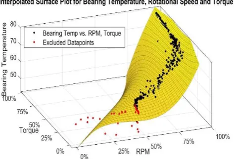
As is the case with many condition monitoring methods, this method is based on building a normal behaviour model. This was achieved through the use of data which was known to be healthy. Using the Matlab Curve Fitting Toolbox, a model was developed for bearing temperature, rotational speed and torque. The temperature function is represented by a polynomial function with three degrees of freedom for rotational speed and two degrees of freedom for torque, as represented by Equation 4 and shown in Figure 2.

𝑇(𝜔, 𝑄) = 𝑝00+ 𝑝10𝜔 + 𝑝01𝑄 + 𝑝20𝜔2+ 𝑝11𝜔𝑄 + 𝑝02𝑄2+ 𝑝30𝜔3+ 𝑝21𝜔2𝑄 + 𝑝12𝜔𝑄2 (4)

Figure 2: Normal behaviour model for bearing temperature, rotational speed and torque

To achieve an accurate result in fitting the surface plot to the data, it was necessary to remove some outliers and data that would cause the normal behaviour model to be wrongly represented. This consisted of data that was captured when the turbine was not generating any power and was removed by setting a threshold to the rotational speed. The removed data is represented by the red data points in Figure 2.

2.4 Standardising Algorithm

The aim of standardising the data was to be able to provide a measure of bearing temperature which also takes into consideration the rotational speed and generator torque. The general method of standardising data is described by equation (2) where the value being standardised has the dataset mean subtracted from it and is then divided by the standard deviation of the dataset. Rather than subtracting the mean of the dataset, this method uses the value obtained from the normal behaviour function. The data is therefore standardised using the Equation 5:

𝑇stan= (𝑇 − 𝑇(𝜔, 𝑄))/𝜎 (5)

where Tstan is the standardised temperature, T is the measured temperature, 𝑇(𝜔, 𝑄) is the healthy temperature obtained from equation (4) and σ is the standard deviation for the healthy temperature dataset.

3 Anomaly Detection

The purpose of standardising in this work is to transform the data into a format which can be used for anomaly detection. Anomaly detection has been defined as the problem of finding patterns in data that do not conform to expected behaviour [12]. By standardising as described above, data which describes normal behaviour will, as expected, have a normal distribution as shown in Figure 4.

Figure 4: Distribution for Normal Behaviour

Therefore as a standardised temperature value is fourther away from zero it increasingly indicates ‘less normal’ behaviour. This characteristic of moving away from the norm will allow anomalies to be detected.

Taking the case of the bearing fault, Figure 5 below shows how the distribution of the data changes in the presence of a fault. In this case the faulty data is ‘standardised’ with the expected value and standard deviation of the healthy data set. As can be seen, in the presence of a fault the distribution of the data has a higher mean and larger standard deviation as compared to the healthy dataset.

Figure 5: Distributions for normal behaviour and one month to failure

To define when a standardised temperature value is abnormal, thresholds can be applied to an estimate of the probability density function as shown in Figure 6.

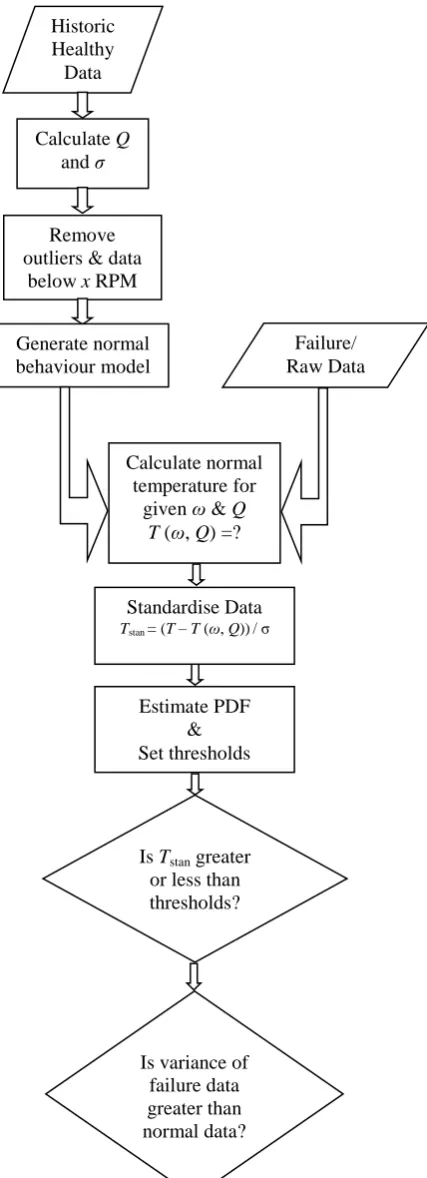
Is Tstan greater or less than thresholds? Historic

Healthy Data

Calculate Q

and σ

Remove outliers & data

below x RPM

Generate normal behaviour model

Calculate normal temperature for

given ω & Q T (ω, Q) =?

Failure/ Raw Data

Standardise Data Tstan = (T – T (ω, Q))/ σ

Estimate PDF & Set thresholds

Figure 3: Standardising methodology flowchart Is variance of

Figure 6: Probability density function showing abnormal thresholds

In this case, we would expect the higher threshold (with a standardised temperature of 0.5) to indicate a fault. The level at which to set the thresholds is an important parameter for the success of the technique in an application setting. If the probability of detecting an anomaly is too high – i.e. the upper standardised threshold is too close to the standardised temperature of 0 – then there is greater chance of false alarms. The thresholds were chosen in this case based on the data being normal when it has a probability greater than 0.01% and abnormal when the probability is less than 0.01%.

4 Results across a Fleet

Analysis using the data standardising method was carried out for the 10 wind turbines described in Section 2.1. Initially a normal behaviour model was used which represented all 10 wind turbines however it was found that although all 10 were of the exact same type and size of machine, there were significant differences between normal operating temperature ranges for each (i.e. mean and standard deviation were significantly different). It was therefore required that a normal behaviour function be generated for each specific wind turbine.

Using the standardising method of analysis, the presence of a fault could be detected in all of the wind turbines analysed. For one turbine it was possible to see the development of the fault two months prior to the failure, as shown in Figure 7, and one month before failure for all of the other cases.

Figure 7: Distribution of data for normal, one month to failure and two months to failure

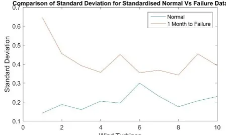
As can be seen from Figure 7, as the fault develops the distribution of data moves in the positive x-axis indicating an increase in temperature. It can also be seen that as the fault develops the standard deviation also increases. Figure 7 is an example in which the presence of the fault can be clearly seen due to the change in both mean and standard deviation, however throughout all of the data analysed the standard deviation is the more reliable indicator of a fault. This increase in standard deviation could be seen for all 10 of the wind turbines analysed as shown in Figure 8. One of way of checking this is through an F-test which checks the null hypothesis that the variance for the distributions of normal and failure data is equal and that the variance of the failure data is greater than the variance of the normal data. As expected this null hypothesis verified that the variance was always higher for the data where a fault was present. F-scores and their changes can be used to statically flag up abnormal failures.

Figure 8: Comparison of standard deviation for normal and failure data

In practice a batch of data may not be available to detect a fault but rather individual data points are assessed in relation to the thresholds shown in Figure 6.

Figure 9: Time series of standardised temperature data for Park 1 Turbine 1

relates to Figure 9 gave a clear indication that a fault was present in the gearbox. There were a few data points classed as normal behaviour but fell above the upper threshold and it may be that the thresholds require adjustment to reduce the likelihood of false alarms.

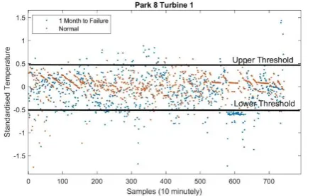
Not all wind turbines gave the same clarity of fault detection as can be seen from the wind turbine represented by Figure 10. The fault in this case doesn’t progress in the same manner as that in Figure 9. In this case it may not be possible to detect the fault until it has developed further and a more obvious increase in standardised temperature is observed. In these cases, the ability to compare samples/batches of recent data by standard deviation is a useful tool.

Figure 10: Time series of standardised temperature data for Park 8 Turbine 1

5 Conclusion

Detecting anomalies within the wind turbine gearbox is made more challenging by the stochastic nature of the wind and the different operating states of the wind turbine. This paper has presented a method of anomaly detection which uses temperature, rotational speed and torque to provide a standardised temperature value which gives a more holistic view of the condition of the gearbox. An expected temperature function for a healthy gearbox (based on a fitted polynomial function in torque and rotational speed) was used as part of the standardised process, along with the standard deviation of the healthy data set. The standardised temperature value allows gearbox anomalies to be detected, either by comparing the statistical properties of sub-populations of data to the healthy data set or by comparing individual data points to systematically chosen thresholds on the standardised temperature distribution.

Although the work in this paper has focussed on detecting a gearbox bearing using the three discussed parameters, the same technique could be applied to other types of faults within the wind turbine gearbox or generator. The success of this detection method is very much dependant on the quality of data used. Large numbers of outliers in the normal behaviour data will reduce the accuracy of the normal behaviour model. This will result in the standardised data being skewed. To avoid this care should be taken to filter out outliers for start-up and shut-down. Care must also be taken

in setting the thresholds as false alarms are detrimental to the overall success of a condition monitoring system.

Acknowledgements

The authors would like to thank the EPSRC Impact Accelerator Account programme at the University of Strathclyde and Offshore Renewable Energy Catapult for funding this work.

References

1. Wind Europe, Wind in power 2017. 2018.

2. van Bussel, G. and C. Schöntag, Operation and Maintenance Aspects of Large Offshore Windfarms. 1997.

3. Hahn, B., M. Durstewitz, and K. Rohrig, Reliability of Wind Turbines, in Wind Energy: Proceedings of the Euromech Colloquium, J. Peinke, P. Schaumann, and S. Barth, Editors. 2007, Springer Berlin Heidelberg: Berlin, Heidelberg. p. 329-332.

4. Guo, P., D. Infield, and X. Yang, Wind turbine generator condition-monitoring using temperature trend analysis. IEEE Transactions on Sustainable Energy, 2012. 3(1): p. 124-133.

5. Zaher, A., et al., Online wind turbine fault detection through automated SCADA data analysis. Wind Energy, 2009. 12(6): p. 574-593.

6. Schlechtingen, M. and I. Ferreira Santos,

Comparative analysis of neural network and regression based condition monitoring approaches for wind turbine fault detection. Mechanical Systems and Signal Processing, 2011. 25(5): p. 1849-1875. 7. Shulian, Y., L. Wenhai, and W. Canlin. The

intelligent fault diagnosis of wind turbine gearbox based on artificial neural network. in 2008 International Conference on Condition Monitoring and Diagnosis. 2008.

8. Schlechtingen, M., I.F. Santos, and S. Achiche, Wind turbine condition monitoring based on SCADA data using normal behavior models. Part 1: System description. Applied Soft Computing, 2013. 13(1): p. 259-270.

9. Jang, J.-S., ANFIS Adaptive-Network-based Fuzzy Inference System. Vol. 23. 1993. 665-685.

10. Yang, W., et al., Wind turbine condition monitoring: technical and commercial challenges. Wind Energy, 2014. 17(5): p. 673-693.

11. Carroll, J., et al., Wind Turbine Gearbox Failure and Remaining Useful Life Prediction Using Machine Learning Techniques. Wiley Wind Energy, Submitted 2017.