Comparative study of non-premixed and partially-premixed combustion simulations in a realistic Tay model combustor

City, University of London Institutional Repository

Citation:

Zhang, K., Ghobadian, A. and Nouri, J. M. (2017). Comparative study of

non-premixed and partially-non-premixed combustion simulations in a realistic Tay model combustor.

Applied Thermal Engineering, 110, pp. 910-920. doi: 10.1016/j.applthermaleng.2016.08.223

This is the accepted version of the paper.

This version of the publication may differ from the final published

version.

Permanent repository link:

http://openaccess.city.ac.uk/15540/

Link to published version:

http://dx.doi.org/10.1016/j.applthermaleng.2016.08.223

Copyright and reuse: City Research Online aims to make research

outputs of City, University of London available to a wider audience.

Copyright and Moral Rights remain with the author(s) and/or copyright

holders. URLs from City Research Online may be freely distributed and

linked to.

City Research Online:

http://openaccess.city.ac.uk/

publications@city.ac.uk

Comparative study of Non-premixed and Partially-premixed combustion

simulations in a realistic Tay model combustor

K. Zhang *

A. Ghobadian

J. M. Nouri

School of Mathematics, Computer Science and Engineering, Department of Mechanical Engineering, City University

London, Northampton Square, London EC1V 0HB, UK.

Keywords: CFD; Combustion Modelling; Gas Turbine Combustor; Non-Premixed Flame; Partially-Premixed Flame

Abstract

A comparative study of two combustion models based on non-premixed assumption and partially premixed assumptions using the overall models of Zimont Turbulent Flame Speed Closure Method (ZTFSC) and Extended Coherent Flamelet Method (ECFM) are conducted through Reynolds stress turbulence modelling of Tay model gas turbine combustor for the first time. The Tay model combustor retains all essential features of a realistic gas turbine combustor. It is seen that the non-premixed combustion model fails to predict the combustion completely due to an incorrect assumption of diffusion flame scenario invoking infinitely fast chemistry in complicated flow environments while the two partially premixed combustion models accurately predict the flame pattern in the primary region of the combustor. The ZTFSC model outperformed the ECFM model by producing a better temperature agreement with the experimental result. The latter model predicts lower temperature due to the underestimation of reaction progress. Additionally, a cross-comparison of the present RSM prediction invoking ZTFSC model with LES prediction reported in the literature is conducted. The former produces more accurate species concentration and flame pattern than the latter. This is mainly due to the incorrect assumption of premixed combustion used in LES prediction reported in the literature. It is interesting to find that when non-premixed combustion model is used for both RSM and LES predictions, the LES predicts higher temperature closer to the injection nozzle of combustor than the RSM model, though the flame shape in both cases is incorrect. This is mainly due to the fact that the traditional RANS model dissipates the energy of swirling flow too fast in the primary region of the combustor. The weaker centre recirculation zone (CRZ) created by vortex breakdown recirculate less air to the area near the injection nozzle resulting in fuel rich combustion. It indicates that the temperature difference between predicted results using RSM in conjunction with ZTFC model and experimental results can be improved by using less energy dissipating turbulence models such as scale resolving simulation (SRS).

1. Introduction

The advent of Gas-Turbine for military purposes tracks back to 1940s, and it is subsequently used for aviation and later for ground level power [1]. The main challenge of aviation industries nowadays is the efficiency, stability of combustion and pollutant control, such as the emission of carbon dioxide (CO2), nitrogen oxide, sulphur dioxide

combustion models which can incorporate detailed chemical reactions are developed under more realistic assumptions.

Due to the complexity of a realistic gas turbine combustor, most researchers focused on performing CFD simulation in a combustor-like burner where fuel and oxidizers are injected separately and no additional oxidizers are injected from other inlets [2-6]. The non-premixed combustion models which employ the infinitely fast chemistry assumptions are commonly used to predict such diffusion flames and are presumed to be an effective model in more complicated flow configuration. While, in a realistic gas turbine combustor, two major complexities make the non-premixed combustion model incorrect: the primary jets which introduce extra oxidizer to premixed mixtures and the extended flame residence time dominated by the strong swirling flow. Hence, the non-premixed combustion models are incorrect propositions when they are used in realistic gas turbine combustors where partially premixed flame occurs due to extra reactants from other inlets.

In a realistic gas turbine combustor, when primary jets introduce extra oxidizers into the premixed mixtures, the local status of premixed mixtures is assumed to be fully burnt if infinitely fast chemistry is assumed. However, in reality, chemical reactions are never infinitely fast. The local reactions amongst mixtures/reactants are only partially progressed which is tracked through the so-called progress variable. Besides, other than the extra oxidizer introduced by primary jets, the cooling airs from porous walls of realistic combustor further reduce the confidence of using non-premixed models. Although the flow rate from the porous wall is relatively low compared to the mainstream, and is commonly assumed not to be involved in any reactions, it is argued that part of these flow is actually brought into self-ignition region by the strong centre recirculation, and they do influence the reactions due to the extended flame residence time. It might be concluded that the more complex the flow configuration is, i.e., with the strong swirling flow and multiple inlet jets, the worse the performance of non-premixed combustion models will be due to the infinitely fast chemistry assumption.

In the past, many researchers have employed non-premixed combustion models to interpret the reactions in realistic gas turbine combustors where partially premixed flame occur. Although some predictions employing non-premixed assumptions are seen in reasonable agreement with experimental results particularly those using large eddy simulation (LES), the flame pattern predicted is incorrect mainly in the primary region where two side flames near the combustor walls are predicted which is inconsistent with experimental result [7-9]. Besides, the use of LES requires huge computational power and is unaffordable for most industrial problems. On the other hand, the far less computational power required Reynolds average Navier-Stoke (RANS) method fails to predict the reacting flow in realistic gas turbine combustors accurately [10]. The principle cause is attributed to the use of the unsuitable non-premixed combustion model rather than the problem of widely used RANS models. In a simple burner, both scale resolving simulation (SRS) and RANS methods are seen to provide acceptable results with the former showing a better agreement [11, 12].

for applying these models to realistic gas turbine combustors.

To compensate for these gaps, a realistic Tay gas turbine combustor which includes complicated features such as fuel injector, swirler, primary holes, dilution holes, discharge nozzle, and porous wall is simulated in this paper. The objectives of the current paper are first to investigate and provide remedies to the deficiencies that have been observed in past simulation[7] of realistic gas turbine combustors, and second to demonstrate an effective and efficient combustion model for predicting realistic gas turbine combustors by comparing the performance of the widely used non-premixed with partially premixed combustion models. The Reynolds stress turbulence model is chosen to solve the mixing problem, and steady laminar flamelet modelling (SLFM) is chosen to simplify chemical reactions. Pre-PDF (probability density function) method is employed for turbulent combustion interaction. To reduce the uncertainties that might be induced by chemistries, 247 chemical reactions and 50 species are employed to represent the full chemistries involved in the combustion of propane [19]. The flame front propagation in the partially premixed combustion model is tracked by solving a transport equation for the density weighted mean reaction progress variable.

2. Mathematical model

In this study, to predict the turbulent combustion in a realistic gas turbine combustor, the Reynolds Stress Model (RSM) is used to describe the mixing problem. The model is seen to provide better performance in simulating the strong swirling flow by abandoning the Boussinesq approximation for 2nd _{order moments and solving six Reynolds}

stress of 𝜏𝑖𝑗 appearing in 3D RANS momentum equations directly. As the main objective of this study is to

investigate the performance of different combustion models in gas turbine combustor where stationary flow assumption can be utilized, the RSM model is chosen for the very fast turn-around and far less computational resources requirements compared to inherently transient methodologies such as LES, DES, and etc.

Non-premixed combustion: In the non-premixed flame, fuel and oxidizer are injected into the combustion

chamber separately. The reaction rate is mainly controlled by the rate of mixing of fuel and oxidizer, and therefore, the generated flame due to this process is also called diffusion flame. The non-premixed combustion is said to be rate limiting process as the regimes of modelling this combustion requires the consideration of both reaction time and mixing time, and which is described by Damkohler number Da = 𝜏𝑡/𝜏𝑐. Poinsot et al. [20] introduced a

regime diagram for non-premixed flame according to the Damkohler number and the turbulence Reynolds number

𝑅𝑒𝑡= 𝑢′𝑙𝑡/𝜈 shown in Fig 1.

The figure divides the turbulent non-premixed combustion problem into three regimes.

A) When the chemical reaction time is much smaller than mixing time, i.e. for fast chemistry, the reactive layer of the flame is assumed to be thinner than the diffusion layer. The smallest Kolmogorov size which is equal to the diffusion layer has no effect on the inner reactive layer, and the turbulent flame is assumed to be composed of laminar flamelets. The flamelet regions are bounded by the flame Damkohler number and the Damkohler number of laminar flamelet assumption (LFA), Da𝑓𝑙_{= 𝐷𝑎}𝐿𝐹𝐴_{. The flame Damkohler number is defined by the ratio of}

flow time scale to chemical time scale, the former can be estimated using the averaged scalar dissipation.

B) For slightly larger chemical time scale, the reactive layer is thickened to the size of Kolmogorov length scale, the LFA is no longer valid, and unsteadiness effect is expected.

C) When the chemical reaction is too slow, the too fast diffusion of the mixture into the reactive layer is not combusted and flame tends to extinguish. The extinction region is bounded by Da = 𝐷𝑎𝑒𝑥𝑡_.

In the present paper, the fast chemistry assumption made in regime A and the steady laminar flamelet method (SLFM) is employed not only in non-premixed combustion but also in partially premixed combustion. The thermochemistry involved in non-premixed combustion is reduced to a single scalar variable, the mixture fraction, denoted by Z. Complete chemical state information can be derived from Z through chemical state relationship, ∅ = ∅(Z) where ∅ can be quantities such as species mass fraction, temperature and density. The presumed probability density function (PDF) is used to account for turbulence–chemistry interaction and is to be discussed in the following sections as well as the discussion on SLFM method.

Partially-premixed Combustion: In the majority of engineering applications, neither pure premixed nor

non-premixed combustion occurs individually. Especially in a realistic gas turbine combustor, the pure consideration of non-premixed combustion has vital defects though the fuel and oxidizer are usually injected to the combustor individually and behaves like diffusion jets. To overcome this problem, a partially premixed combustion model is employed by combining the premixed and non-premixed combustion models. The injected fuel and oxidizers in the combustor are only classified by their two statuses, either combusted or not combusted. For the combusted burnt mixtures, the regime A in non-premixed combustion model can be employed to decide the properties of the flame. For unburnt mixtures, the simple mixing problem can be easily solved without reactions. The only question is how to solve the status of local mixtures. An extra transport equation for the so-called reaction progress variable can be employed to track the position of the flame front. The method has been used in premixed combustion models for many years.

In partially premixed combustion mode, the progress variable is essentially used to compensate the deficiencies of mixture fraction theory as the mixture fraction does not contain any intrinsic information about the progress of chemical reactions. The local status of the mixtures is mainly distinguished by the amount of reactions progressed. The transport equations of the progress variable and mixture fraction are shown in equation 1.

{

𝜕𝜌𝑍

𝜕𝑡 + ∇ ∙ (𝜌𝑢𝑘𝑍) = ∇ ∙ (ρ𝛼𝑧∇𝑍) 𝜕𝜌𝐶

𝜕𝑡 + ∇ ∙ (𝜌𝑢𝑘𝐶) = ∇ ∙ (ρ𝛼𝑐∇𝐶) + 𝜌𝜔𝑐

(1)

Where 𝛼𝑧= 𝜇𝑡/𝜎𝑡, and the turbulent Prandtl number 𝜎𝑡 takes the value of 0.85, 𝛼𝒄= 𝜇𝑡/𝑆𝑐𝑡 and the turbulent

a thin flame can then be calculated as in equation 2.

∅ = C ∫ ∅₀1 𝑏(𝑍)𝑝(𝑍)𝑑𝑍 + (1 − 𝐶) ∫ ∅₀1 𝑢(𝑍)𝑝(𝑍)𝑑𝑍 (2)

Where 𝑝(𝑍) represents the presumed PDF (see equation 25). When C=1, mixtures are burnt so that the regime A in non-premixed combustion is adopted, when C=0, purely mixing problem is solved using mixture fraction theory. While, when mixture is fully burnt (C=1), as the strained steady laminar flamelet method has been used for current study, the density weighted scalar quantities are not only a function of mixture fraction, but also a function of scalar dissipation/strain rate as shown in equation 8. Besides, in order to solve the progress variable in equation 1, modelling must be provided to the reaction progress term 𝜔𝑐 (which is also called mean reaction rate).

Five regimes as shown in Fig 2 have been proposed to describe the behaviour of the flame front under the impact of turbulence and chemical reactions. In this paper, two regimes are employed to provide closure to the term 𝜔𝑐,

the Zimont Turbulent Flame Speed Closure Method and extended coherent flamelet method.

Fig. 2 Regime diagram for premixed combustion. [21]

Zimont Turbulent Flame Speed Closure (ZTFSC) Method: The mean reaction rate in equation 1 can be modelled

as [22]:

𝜌𝜔𝑐= 𝜌𝑢𝑈𝑡|∇𝐶| (3) Where 𝜌𝑢 is the density of unburnt mixture and 𝑈𝑡 is the turbulent flame speed which must be evaluated. The

ZTFSC model belongs to the group of turbulent flame speed (TFS) methods. There are many other models to decide the TFS, but are not used here [23].

The ZTFSC method computes the turbulent flame speed by considering the wrinkled and thickened flame front and the regime used locates in the region of thin reaction zones in Figure 2.The thin reaction zone regime assumes that the smallest Kolmogorov size is smaller than the diffusion layer and penetrates to the flame zone, but is still larger than the reactive layer, so the theory of laminar flamelet still applies. The thin reaction zone is quantified by Karlovitz number, Ka, larger than unity and Ka is defined as the ratio between the flame time scale and Kolmogorov time scale. The ZTFSC method computes the turbulent flame speed by:

Where A takes the value of 0.52 recommended in [22], 𝑢′ _{represents root mean square (RMS) velocity. 𝑈} 𝑙, the

laminar flame speed can be calculated either based on the proposed correlation by Metghachi and Keck [24] or from fitted curve achieved from the simulation of the laminar flame speed [25]. The latter is used in the present paper. The α in the equation 4 is the molecular heat transfer coefficient of the unburnt mixture, and 𝑙𝑡 is the

turbulent length scale calculated from 𝑙𝑡= 𝐶𝐷𝑘3/2/𝜀 where 𝐶𝐷 equals 0.37, 𝑘 represents turbulent kinetic energy

and 𝜀 represents turbulence dissipation rate. The regime used by ZTFSC model is also called Intermediate Steady Propagation (ISP) combustion regime that the flame front consumes fuel at the speed proportional to the ratio between turbulent time scale 𝜏𝑡= 𝑙𝑡/𝑢′ and chemical time scale 𝜏𝑐= α/𝑈𝑙2. The stretch effect is considered by

ZTFSC model by multiplying 𝜌𝜔𝑐, the mean reaction term with a probability stretch factor G and details are not

discussed here, but could be found in [26].

Extended Coherent Flamelet Method (ECFM): Having discussed the thin reaction zone regime used in ZTFSC

model, it is interesting to consider the region where Ka is smaller than unity in Fig 2. Two regimes of wrinkled and corrugated flamelets exist in this region and ECFM model is used to account for flame front corrugation by involving a transport equation of flame area density, denoted by Σ. For wrinkled flamelets regime, the ratio of the local turbulence velocity fluctuation to laminar flame speed is smaller than unity, indicating that turbulent eddies are unable to deform the flame front, and only slight wrinkling could occur. While this is not practical as in most engineering applications, the turbulent intensity is relatively large. The ratio of local turbulence velocity fluctuation to laminar flame speed is larger than one and the flame front is corrugated. In both of the two regimes, the smallest eddies are assumed to be larger than flame front thickness so the effect of turbulence is to wrinkle or corrugate the laminar flame sheet. As the reactive layer of the flame is not perturbed by the smallest eddies, the flame is quasi-laminar and theory of laminar flamelets applies.

The increased flame area due to wrinkling increases the fuel assumption rate and flame speed, so a transport equation of flame area density in equation 5 is needed to track their effect [27].

𝜕𝜌Σ

𝜕𝑡 + ∇ ∙ (𝜌𝑢𝑘Σ) = ∇ ∙ (ρ𝛼Σ∇Σ) + 𝑆Σ (5)

Where 𝛼Σ= 𝜇𝑡/𝑆𝑐𝑡 and the turbulent Schmidt number 𝑆𝑐𝑡takes the value of 0.7. The 𝑆Σ is composed of four

production terms and one dissipation term but the details are not provided here. Various models are proposed to close these terms, and the closure method provided by Colin et al. [28] is employed in this paper. The computed flame area density is then used to provide closure to the reaction progress term 𝜔𝑐 in equation 1:

𝜌𝜔𝑐= 𝜌𝑢𝑈𝑙Σ (6)

Steady Laminar Flamelet Method (SLFM): As it has been discussed above, the SLFM is suitable for both the

ECFM and ZTFSC models. The basic concept of this method views the turbulent flames as an ensemble of 1D-thin, laminar flamelets embedded in the turbulent flow field [23, 29-30]. Therefore, the concept is only applicable when the smallest Kolmogorov eddies in the flow field are assumed to be larger than the reactive layer of the flame.

The strain rate can be defined as 𝑎𝑠= 𝑣/2𝑑, but is often replaced by the scalar dissipation represented as:

X = 2D|∇Z|2 ₍₇₎

Where D is the diffusion coefficient. The equation defines the scalar dissipation as a function of diffusion rate and gradient of mixture fraction. A zero scalar dissipation represents the status of chemical equilibrium. The general laminar counterflow diffusion flame equations can be described in the mixture fraction space transformed from the physical space by:

{ 𝜌

𝜕𝑌_𝑖 𝜕𝑡 =

1 2𝜌𝑋

𝜕2_𝑌 𝑖

𝜕𝑍2+ 𝜔̇𝑖

𝜌𝜕𝑇_𝜕𝑡−1₂𝜌𝑋𝜕_𝜕𝑍2𝑇2−

1

𝐶𝑝∑ 𝐻𝑖 𝑖𝜔𝑖̇ −

1 2𝐶𝑝𝜌𝑋

𝜕𝐶𝑝𝜕𝑇

𝜕𝑍2 −

1

2𝐶𝑝𝜌𝑋 ∑ 𝐶𝑝,𝑖

𝜕𝑌𝑖𝜕𝑇

𝜕𝑍2

𝑖 = 0

(8)

Where 𝑌𝑖 is the ith species mass fraction, 𝐶𝑝,𝑖 and 𝐶𝑝 are the specific heat of ith species and the mixtures. 𝐻𝑖 and 𝜔̇𝑖

are the specific enthalpy and species reaction rate for the ith _species.

In an SLFM approach, the first term on the L.H.S. of equation 8 disappears. The approach is strictly applicable to fast chemical reactions and turbulence induced chemical non-equilibrium is mainly due to aerodynamic strain. By employing this approach, the 247 chemical reactions and 50 species detailed chemical reactions [19] employed in this study can be used to calculate the laminar opposed-flow diffusion flame in the mixture fraction space. The steady laminar flamelets are tabulated beforehand considering the full scalar dissipation rate from chemical equilibrium of 0/s to flame extinction of 58/s for accuracy purpose and to avoid high computational power required in solving species in physical space.

Presumed Probability Density Function (Presumed-PDF):

In order to account for the turbulence-chemistry interaction, a Presumed-PDF method is employed. The method considers the fluctuation of local mixture fraction by the turbulence through the mixture variance 𝑍′2_{by employing}

analytical solution of Beta-function:

P(Z) =Γ(𝑎+𝑏)𝑍_Γ(a)Γ(b)𝑎−1(1−𝑍)𝑏−1 (9)

Where Γ is the gamma function, a and b are PDF parameters expressed as:

{ 𝑎 = 𝑍[

𝑍(1−𝑍) 𝑍′2 − 1]

𝑏 = (1 − 𝑍)[𝑍(1−𝑍)_𝑍′2 − 1]

(10)

To determine the probability function, an additional transport equation for mixture fraction variance 𝑍′2 _{must be}

given:

𝜕 𝜕𝑡(𝜌𝑍

′2_{) + ∇ ∙ (𝜌𝑢}

𝑘𝑍′2) = ∇ ∙ (𝛼z′∇𝑍′2) + 𝐶𝑔𝜇𝑡(∇Z)2− 𝜌𝑋 (11)

Where 𝛼z′= 𝜇𝑡/𝜎𝑡 and model constants 𝜎𝑡(Prandtl number), 𝐶𝑔 are defined to be 0.85 and 2.86. 𝑋 = 𝐶𝑑𝑍′2𝜀/𝑘

3. Solution methods

In this study, the segregated semi-implicit algorithm simple method is used for pressure-velocity coupling scheme. Transport equations, which are density weighted, are solved by commercial CFD code, Ansys Fluent 14.5 (Finite volume method based) [32]. Hexahedral rather than tetrahedral mesh is constructed through Ansys ICEM to improve the accuracy of prediction. Grid independence is checked by mesh refinement strategy and three mesh densities of 0.7, 1.2 and 2 million are tested that the last one of 2 million meshes is chosen for present study to ensure the highest accuracy. Second order upwind is applied to the momentum, progress variable, mean mixture fraction, mixture fraction variance as spatial discretization method [33].

Experiment Simulated:

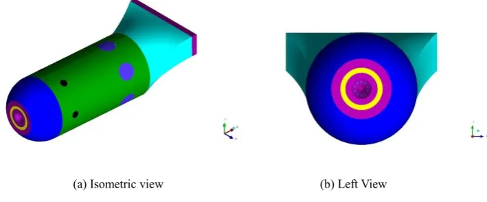
Fig. 3 shows the configuration of the model can type combustor described in Bicen, Tse and Whitelaw [34]. It represents a realistic industrial Tay combustor retaining the essential components of the hemispherical head (blue), cylindrical barrel (green), circular to rectangular discharge nozzle (cyan), swirler (yellow), fuel device, primary holes (black) and secondary/dilution holes (purple). The wall of the combustor including head, barrel, and discharge nozzle are made of ‘Transply’, a kind of porous material.

According to the experiment, six primary holes and six dilution holes are equally distributed around the cylindrical barrel with the former having a diameter of 10mm, and the latter 20mm. However, it was shown that the radial velocity profile of flow through primary holes has a tremendous impact on the flow field in the primary region. Different peak values instead of the plug flow assumptions of radial velocity in the hole affect the central part of combustor by promoting a stronger penetration of the jets. It was recommended by McGuirk and Palma [35] that an artifice such as the reduction of the hole diameter by 14% corresponding to the discharge coefficient CD of 0.74

seems to be a good compromise in case no reasonable guess can be made about the shape of the profile. The use of reduced diameter from 10mm to 8.6mm decreases the maximum axial velocity at a position closer to injection nozzle and provides better velocity agreement with the experimental data. The swirler, mounted on the hemispherical head, comprises 18 curved vanes and each of them was originally designed with a thickness of 0.56mm. To reduce the complexity of meshing, swirler vanes are not created. Instead, annular shape of swirler (yellow) is used that the effective area at the swirler exit is computed and axial velocity component is determined from the datum swirler exit area. The tangential velocity is obtained by taking into account of turning efficiency of the vanes and blockage effects following the procedures of determining swirler boundary conditions suggested in

[36, 37]:

ω = η 𝑊𝑠𝑤

𝐴𝑠𝑒𝜌𝐶𝑑(1−𝑏)𝑡𝑎𝑛𝛼 (12)

Where the blockage factor is taken as 0.1, and the turning efficiency is 0.92. Value of 0.75 is assigned to the discharge coefficient, 𝐶𝑑. The flow characteristics of the swirler used in the original experiment and this prediction

is available in the technical paper of Bicen and Palma [38].

The propane fueling device has 10, 1.7mm diameter holes equally distributed on a central cone section shown in

(a) Isometric view (b) Left View

Fig. 3 Configuration of model can type combustor

A summary of the experimental conditions used in this prediction is given in Table 1. According to the experiment, 6.9% of total air was injected through swirler, 13.6% through primary holes and 53.3% through dilution holes into the combustor. To simplify the porous media problem, fixed mass flow rate of 6.6% of total air is assigned to the hemispherical head (blue), 13.8% to the cylindrical barrel (green), and 5.8% to circular to the rectangular discharge nozzle (cyan).

Table 1 Experimental condition

Exp ma

(g/s)

mg

(g/s)

Swirler Vane Angle

P

(atm)

Tinlet

(K)

AFR

1 100 1.76 45 1 315 57

The computation of the current study was carried out on a 20 processing element solon cluster at City University London. The steady RSM model based simulation greatly reduces the computational time that total wall clock time of around 10 hours are spent for one prediction (2 million mesh). The past prediction based on LES requires total wall clock time of 26,432 hours using 64 processing elements of Cray T3E at the University of Manchester is unaffordable by most industries (1 million mesh) though the prediction is done in 2004 [7].

4. Result and Discussion

4.1 Behaviour of flow field and scalar variables

(a) (b)

(c)

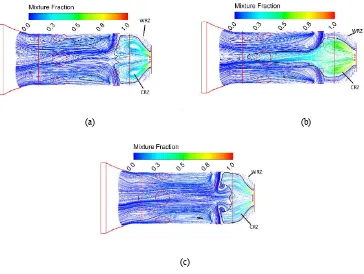
Fig. 4 Streamline of flow field coloured by mixture fraction. (a) ZTFSC model, (b) Non-premixed model, (c) ECFM model. Black solid line: stoichiometric mixture fraction=0.0639.

Although two results from the partially premixed combustion models of ZTFSC and ECFM show a similar distribution of mixture fraction in the primary region, differences between them are noticed as well. The predicted size of CRZ using ECFM model is seen to be much smaller than the one predicted by ZTFSC model. As the energy trapped in the CRZ is initially generated by swirling jets, smaller CRZ may indicate higher angular momentum but lower axial momentum. With lower axial momentum, the CRZ is not penetrating to the downstream and stopped by primary jets. Instead, two smaller vortices are formed just after the CRZ due to the high lateral momentum of primary jets. On the other hand, with higher angular momentum, the increased intensity of CRZ has trapped more fuels in the primary region leading to a lower mixture fraction in the secondary zone (Disappear of the black solid line). The intensity of CRZ in the primary region is simply represented by the vorticity of the flow shown in Fig 5. The highly swirling core (HSC) is broken up for the prediction using ZTFSC model, while the result from ECFM preserves the HSC indicating higher angular momentum. The preserved HSC from ECFM model is believed to have increased the stability of flame.

In addition, as the main objective of this paper is to demonstrate the performance of different combustion models in a realistic combustor, more focuses are put on the performance of non-premixed combustion model in Fig 4b

(a) (b)

Fig. 5 Intensity of CRZ in primary region represented by vorticity = 9776.83/s for (a) ZTFSC model, (b) ECFM model.

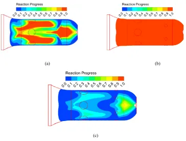
Fig 6 shows the progress variable (reaction progress) contour for all three combustion models. The reaction progress of unity indicates the local mixtures are fully combusted while the reaction progress of zero represents no reaction. In non-premixed combustion, whenever the fuel meets with the oxidizer, combustion completed immediately within the flammability limit. The reactions are said to be fully progressed under this condition and the progress variable is assigned to be unity implicitly. While, the prediction by ZTFSC model has limited the reaction progress in the region closer to the porous wall where cold jets extinguish the flame. Attentions are given to the performance of ECFM model that the reactions in the primary region are greatly limited probably due to the underprediction of the strength of turbulence.

(a) (b)

(c)

Fig. 6 Progress variable (reaction progress) contour. (a) ZTFSC model, (b) Non-premixed model, (c) ECFM model.

from porous walls. While predicted flame by non-premixed combustion penetrate to the downstream of the combustor that the flame temperature near the secondary holes is much higher than the temperature in the primary zone (incomplete combustion in the primary zone). Not surprised that due to the limited reaction progressed predicted by ECFM model, the combustion is not properly captured though the highest temperature occurs in the primary region of combustor shown in Fig 7c.

(a)

(b)

(c)

In Fig 8, the predicted temperature by Di Mare et al. [7] using large eddy simulation (LES) and non-premixed combustion model is compared with the result by using partially premixed and RSM model in this study. Although large temperature difference near the combustor walls is observed that Fig 8b has two side flames compared to Fig 8a, the flame of highest temperature is similar. Regardless of the turbulence models used, the main reason for this differences can only be caused by the combustion models chosen.

(a) (b)

Fig. 8 Temperture in the primary zone: horizontal midplane. (a) ZTFSC & RSM model, (b) LES & Non-premixed model, Colour scale: five levels between pink = 2200K and blue = 315K [7].

By observing Fig 6a and b at the position where two side flames occur, the ZTFSC model presents much lower progress variable of around 0.20.3 compared to the non-premixed combustion model. Such a low value of progress variable indicates the unburnt or partially burnt nature of local mixtures. The statistical comparisons of the temperature and species concentration with experimental results are presented in the following section. The two side flames are confirmed to be non-existent illustrating the importance of employing partially premixed assumptions in complicated flow environment.

4.2 Statistical Results

In this section, the statistical results of the computation are discussed and compared with measurement [33], as well as the prediction by Di Mare et al. [7]. Because of limited information about the shape of circular to rectangular part at downstream of the combustor, only statistical result in the primary region is used for comparison. The flame in the primary region is of the most interest to most researchers due to the complicated multi-jets, highly swirling flow condition. The proper prediction of the flame in this region will usually indicate a good estimation in the downstream of the combustor.

attributed to its ability to account for the imperfect/slow mixing of fuel and swirler air as well as the addition of air through other routes such as porous wall and primary holes.

By comparing the result from Di Mare et al. [7] and the non-premixed prediction from our result, the temperature difference can only be attributed to the different turbulence models employed in the predictions. It is widely accepted that LES model is less dissipative and less energy of CRZ will be dissipated compared to RANS model used in our prediction. It is believed that the more intensive CRZ allows the unburned fuel to be recirculated back to upstream for further combustion and will certainly improve the local temperature.

(a) (b)

(c)

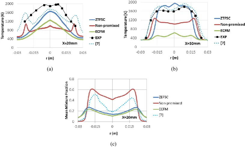
Fig. 9 Profile of temperature and mixture fraction in the horizontal midplane of the combustor.

Due to the fact that the CRZ predicted by RANS model is less intensive due to over prediction of mixing, more fuel is held near the primary holes without being recirculated to the upstream of the combustor. This extra amount of fuel mixes with oxidizers thoroughly allowing the combustion to happen at approximately stoichiometric mixture fraction. Meanwhile, insufficient oxidizers from primary holes are recirculated to the upstream of primary region resulting in fuel rich combustion at x=20mm. Therefore, the temperature predicted by RANS model is seen to be higher than the one by LES [7] shown in Fig 9b. In addition, in Fig 9c, the mean mixture fraction predicted by the two partially premixed combustion models are seen to be the same, the temperature differences predicted can only be caused by the underestimation of progress variable by ECFM model shown in Fig 6.

(a) (b)

(c) (d)

Fig. 10 Profile of species mole fraction in the horizontal midplane of combustor (x=20mm).

Although the prediction of oxygen mole fraction is seen to be far from experimental result, with more consumption of propane at a radial position of 0.0225m, the mole fraction of oxygen will be in reasonable agreement with experimental result, i.e. there is an underprediction of combustion near the injection nozzle, shown in Fig 6a.

Finally, the prediction of carbon monoxide in Fig 10b is problematic that none of the available models properly captures its profile. It was concluded by Di Mare et al. [7] that the CO level may not be well represented by steady laminar flamelet method due to its slower reaction rate. All the other species other than carbon monoxide are less sensitive to this and are more strongly influenced by transport effects. As 247 chemical reaction, 50 species and full scalar dissipation rate are employed in our prediction, it confirms the conclusion made in Di Mare et al. [7]

that more detailed reaction mechanism and the consideration of strain effects have little influence on the prediction of CO concentration.

5. Conclusions:

Comparative studies of the partially premixed and non-premixed combustion models have been presented. The chosen geometry retained all features of a commercial aviation used can-type combustor and provides an excellent test case to illustrate the effectiveness of using well coupled partially premixed combustion model in complicated, three-dimensional, multi-jets swirling flow environment. The RSM model is used to solve the mixing problem. Tabulated chemistry and SLFM are chosen to simplify the employed detailed chemical reactions and to reduce the computational time. Pre-PDF method is used for turbulent combustion interaction. The main findings of the present papers are:

 For the first time, the partially premixed combustion model has been applied to a Tay model combustor

and the performance is seen to be completely different from that predicted by non-premixed combustion

in a simple burner, far less attention has been focused on the performance of two models in complicated

flow structures.

 It is noticed that although the use of RSM and non-premixed combustion model fails to predict the

combustion in complicated flow configuration completely, the use of LES does improve the result at the

position closer to the primary jets of combustor. However, both LES and RSM models fail to predict

flame pattern and species concentration based on non-premixed combustion model near the injection

nozzle.

 For the first time, the comparative study of two partially combustion models of ZTFSC and ECFM is

performed in the Tay model combustor. The predicted mixture fraction by ZTFSC model is similar with

that predicted by ECFM in the primary region of the combustor, while the latter model predicts much

lower temperature due to the underprediction of reaction progress. Both models predict the flame shape

reasonably more accurate in the primary region as compared to the non-premixed combustion

predictions regardless of whether RANS or LES is used.

 The temperature and species concentration predicted by the RSM model in conjunction with ZTFSC

model are in reasonable agreement with the experimental result. Although there is still temperature

difference between the prediction and the experimental result, the flame pattern is accurately captured.

The use of SRS models such as LES will compensate for this defects though not presented in this paper.

 The predicted species concentration of fuel, O2 and CO2 are in reasonable agreement with experimental

results while CO concentration may not be well captured by SLFM method. All the other species other

than CO are less sensitive to SLFM method and are more strongly influenced by transport effects. More

detailed reaction mechanism and the full consideration of strain effects have little influence on the

prediction of CO concentration.

Finally, it is concluded that a more realistic assumption based on partially premixed combustion model must be properly coupled with either RANS or SRS turbulence models in order to predict the combustion in a complicated flow environment (such as Tay combustor) efficiently and accurately. In current study, for the first time, the coupling of a RSM turbulence model with ZTFSC combustion model invoking tabulated chemistry successfully predicts the combustion in the Tay model combustor within 10 hours by a 20 processing elements of Solon cluster at City University London (2 million mesh), while the excessive time of 26,432 hours by coupling LES with a non-premixed combustion model using 64 processing elements of Cray T3E at University of Manchester is unaffordable by most industries (1 million mesh) [7].

Acknowledgements The authors would like to thank the City University London for partial financial support for this research.

References:

[2] Wang, P., Fröhlich, J., Maas, U., He, Z.X. and Wang, C.J., 2015. A detailed comparison of two sub-grid scale combustion models via large eddy simulation of the PRECCINSTA gas turbine model combustor. Combustion and Flame.

[3] Liu, Y., Tang, H., Tian, Z. and Zheng, H., 2015. CFD Simulations of turbulent flows in a Twin Swirl Combustor by RANS and Hybrid RANS/LES Methods. Energy Procedia, 66, pp.329-332.

[4] Philip, M., Boileau, M., Vicquelin, R., Riber, E., Schmitt, T., Cuenot, B., Durox, D. and Candel, S., 2015. Large Eddy Simulations of the ignition sequence of an annular multiple-injector combustor. Proceedings of the

Combustion Institute, 35(3), pp.3159-3166.

[5] İlbaş, M., Karyeyen, S. and Özdemir, İ., 2015. Investigation of premixed hydrogen flames in confined/unconfined combustors: A numerical study. International Journal of Hydrogen Energy, 40(34), pp.11189-11194.

[6] Li, S., Zheng, Y., Zhu, M., Martinez, D.M. and Jiang, X., 2015. Large-eddy simulation of flow and combustion dynamics in a lean partially premixed swirling combustor. Journal of the Energy Institute.

[7] Di Mare, F., Jones, W.P. and Menzies, K.R., 2004. Large eddy simulation of a model gas turbine combustor.

Combustion and Flame, 137(3), pp.278-294.

[8] Di Mare, F. 2002. Large eddy simulation of reacting and non-reacting turbulent flows. PHD thesis. Department of Mechanical Engineering, Imperial College London.

[9] Jones, W.P., 2002. Large eddy simulation of turbulent combustion processes. Computer Physics

Communications, 147(1), pp.533-537.

[10] Krieger, G.C., Campos, A.P.V., Takehara, M.D.B., da Cunha, F.A. and Veras, C.G., 2015. Numerical simulation of oxy-fuel combustion for gas turbine applications. Applied Thermal Engineering, 78, pp.471-481. [11] Yang, Z., Li, X., Feng, Z. and Chen, L., 2016. Influence of mixing model constant on local extinction effects and temperature prediction in LES for non-premixed swirling diffusion flames. Applied Thermal Engineering, 103, pp.243-251.

[12] Ziani, L., Chaker, A., Chetehouna, K., Malek, A. and Mahmah, B., 2013. Numerical simulations of non-premixed turbulent combustion of CH 4–H 2 mixtures using the PDF approach. International Journal of Hydrogen

Energy, 38(20), pp.8597-8603.

[13] Baudoin, E., Bai, X.S., Yan, B., Liu, C., Yu, R., Lantz, A., Hosseini, S.M., Li, B., Elbaz, A., Sami, M. and Li, Z.S., 2013. Effect of partial premixing on stabilization and local extinction of turbulent methane/air flames. Flow,

turbulence and combustion, 90(2), pp.269-284.

[14] Bajaj, P. 2001. NOx Reduction in Partially Premixed Combustion. PHD thesis. Technical University of Stuttgart.

[15] Ramaekers, W.J.S., Albrecht, B.A., van Oijen, J.A., de Goey, L.P.H. and Eggels, R.G.L.M., 2005. The application of flamelet generated manifolds in modelling of turbulent partially premixed flames. RGLM Eggels. [16] Chrigui, M., Gounder, J., Sadiki, A., Masri, A.R. and Janicka, J., 2012. Partially premixed reacting acetone spray using LES and FGM tabulated chemistry. Combustion and flame, 159(8), pp.2718-2741.

[17] Andreini, A., Bertini, D., Facchini, B. and Puggelli, S., 2015. Large-Eddy Simulation of a Turbulent Spray Flame Using the Flamelet Generated Manifold Approach. Energy Procedia, 82, pp.395-401.

[18] Kuenne, G., Ketelheun, A. and Janicka, J., 2011. LES modeling of premixed combustion using a thickened flame approach coupled with FGM tabulated chemistry. Combustion and Flame, 158(9), pp.1750-1767.

[19] Chemical-Kinetic Mechanisms for Combustion Applications", San Diego Mechanism web page, Mechanical and Aerospace Engineering (Combustion Research), University of California at San Diego (http://combustion.ucsd.edu).

[21] Peters, N., 1999. The turbulent burning velocity for large-scale and small-scale turbulence. Journal of Fluid mechanics, 384, pp.107-132.

[22] Zimont, V., Polifke, W., Bettelini, M. and Weisenstein, W., 1997, June. An efficient computational model for premixed turbulent combustion at high Reynolds numbers based on a turbulent flame speed closure. In ASME 1997 International Gas Turbine and Aeroengine Congress and Exhibition (pp. V002T06A054-V002T06A054). American Society of Mechanical Engineers.

[23] Bray, K.N.C. and Peters, N., 1994. Laminar flamelets in turbulent flames. Turbulent reacting flows, pp.63-113.

[24] Metghalchi, M. and Keck, J.C., 1982. Burning velocities of mixtures of air with methanol, isooctane, and indolene at high pressure and temperature. Combustion and flame, 48, pp.191-210.

[25] Göttgens, J., Mauss, F. and Peters, N., 1992, December. Analytic approximations of burning velocities and flame thicknesses of lean hydrogen, methane, ethylene, ethane, acetylene, and propane flames. In Symposium (International) on Combustion (Vol. 24, No. 1, pp. 129-135). Elsevier.

[26] Zimont, V.L. and Lipatnikov, A.N., 1995. A numerical model of premixed turbulent combustion of gases. Chem. Phys. Rep, 14(7), pp.993-1025.

[27] Candel, S.M. and Poinsot, T.J., 1990. Flame stretch and the balance equation for the flame area. Combustion Science and Technology, 70(1-3), pp.1-15.

[28] Colin, O., Benkenida, A. and Angelberger, C., 2003. 3D modeling of mixing, ignition and combustion phenomena in highly stratified gasoline engines. Oil & gas science and technology, 58(1), pp.47-62.

[29] Peters, N., 1984. Laminar diffusion flamelet models in non-premixed turbulent combustion. Progress in energy and combustion science, 10(3), pp.319-339.

[30] Peters, N., 1988, December. Laminar flamelet concepts in turbulent combustion. In Symposium (International) on Combustion (Vol. 21, No. 1, pp. 1231-1250). Elsevier.

[31] Spalding, D.B., 1971, December. Mixing and chemical reaction in steady confined turbulent flames. In Symposium (International) on Combustion (Vol. 13, No. 1, pp. 649-657). Elsevier.

[32] ANSYS® , Academic Research, Release 14.5.

[33] Barth, T.J. and Jespersen, D.C., 1989. The design and application of upwind schemes on unstructured meshes. [34] Bicen, A.F., Tse, D.G.N. and Whitelaw, J.H., 1990. Combustion characteristics of a model can-type combustor. combustion and Flame, 80(2), pp.111-125.

[35] McGuirk, J.J. and Palma, J.L., 1992. The influence of numerical parameters in the calculation of gas turbine combustor flows. Computer methods in applied mechanics and engineering, 96(1), pp.65-92.

[36] Crocker, D.S., Fuller, E.J. and Smith, C.E., 1997. Fuel nozzle aerodynamic design using CFD analysis. Journal of engineering for gas turbines and power, 119(3), pp.527-534.

[37] Lefebvre, A.H., 1983. Gas Turbine CombustionMcGraw-Hill. New York, pp.492-495.