Observations on the ponderomotive force

Observations on the ponderomotive force

D.A. Burton

_{, R.A. Cairns}

_{, B. Ersfeld}

_{, A. Noble}

_{, S. Yoffe}

_{, and D.A. Jaroszynski}

a

_{University of Lancaster, Physics Department, Lancaster LA1 4YB, UK}

b

_{University of St Andrews, School of Mathematics and Statistics, St Andrews KY16 9SS, UK}

_{University of Strathclyde, Department of Physics, Glasgow G4 0NG, UK}

ABSTRACT

The ponderomotive force is an important concept in plasma physics and, in particular, plays an important role in many aspects of the theory of laser plasma interactions including current concerns like wakefield acceleration and Raman amplification. The most familiar form of this gives a force on a charged particle that is proportional to the slowly varying gradient of the intensity of a high frequency electromagnetic field and directed down the intensity gradiant. For a field amplitude simply oscillating in time there is a simple derivation of this formula, but in the more general case of a travelling wave the problem is more difficult. Over the years there has been much work on this using Hamiltonian or Lagrangian averaging techniques, but little or no investigation of how well these theories work. Here we look at the very basic problem of a particle entering a region with a monotonically increasing electrostatic field amplitude and being reflected. We show that the equation of motion derived from a widely quoted ponderomotive potential only agrees with the numerically computed orbit within a restricted parameter range and that outside this range it shows features which are inconsistent with any ponderomotive potential quadratic in the field amplitude. Since the ponderomotive force plays a fundamental role in a variety of problems in plasma physics we think that it is important to point out that even in the simplest of configurations standard theories may not be accurate.

Keywords: Laser plasma, ponderomotive force

1. INTRODUCTION

The ponderomotive force, produced by a high frequency electromagnetic field whose intensity varies in space over a scale length long compared to the particle oscillation amplitude in the wave, is a fundamental concept in plasma physics that is widely used when considering laser-plasma interactions, but is by no means confined to this part of the subject. With an electric field of the form

E=E0(r) cos(ωt) (1)

the familiar form of the ponderomotive force is

F =−1 4

q2

mω2∇E 2

0 (2)

where q and m are the particle charge and mass respectively. This formula holds for both electrostatic and electromagnetic waves, but here we will be concerned only with longitudinal waves with the field and the spatial variation of its amplitude in thexdirection, for which a simple derivation of the formula can be given as follows. Neglecting the spatial variation of the amplitude, the displacement of the particle from its mean positionx0due

to the wave is given by

x−x0=−

qE0

mω2cos(ωt) (3)

and if we now take account of the spatial variation by making the approximation

E(x, t) =

E0(x0) + (x−x0)

dE0

dx

use (3) and take the time average we get (2).

If we have a travelling wave withE=E0(x) cos(kx−ωt) then the problem becomes more difficult since there

is no simple solution for the particle displacement. One obvious way forward is to take the local solution

x=x0+V t+ξ (5)

withV an average velocity only varying over the long length scale, then neglectξin the argument of the cosine. This leads to

ξ=− q

m(ω−kV)2E (6)

and, if the procedure above is followed, an average force on the particle of −1 4

q2 m(ω−kV)2∇E

2

0.1 However, as

we shall see this is not a good approximation and later work concentrated on obtaining the force by more sophisticated Hamiltonian or Lagrangian methods.2–5 _{These references are just a sample from a very extensive} literature on the subject, from which we will concentrate particularly on the work of Bauer, Mulser and Steeb4 since it gives an explicit formula relevant to our problem. The argument leading to their expression can be paraphrased as follows. With a displacementξ, the resultant change in potential energy is -ξEand if we assume

ξ=− q

m(ω−kV)2E0cos(kV t−ωt) (7)

E=E0cos(kV t−ωt) (8)

the average potential energy becomes1 2

q2 m(ω−kV)2E

2

0 and the average kinetic energy due to the oscillatory motion

is half of m₂ qE0

m(ω−kV)

2

. The result is an average Lagrangian

L= 1 2mV

2₋1

4 q2

m(ω−kV)2E 2

0. (9)

The standard Lagrange equation is now used to obtain the variation over the long time and space scales, the result being

mdV dt =−

q2

4m

(ω−kV)(ω−3kV)

(ω−kV)4₋3 2

q2

m2k2E2

dE2 0

dx . (10)

Clearly there are approximations involved in the calculation of the average potential and kinetic energy, the assumed particle displacement and velocity not being exact, so the question arises as to how well this formula works. Despite the fact that it is a simple matter to integrate the equation for the exact particle orbit in the field we describe, little or no work has, so far as we know, been done to verify the accuracy of the various expressions for the ponderomotive force that have appeared in the literature. We shall do this for the very basic case of a particle moving in an electrostatic travelling wave with a monotonic intensity profile and show that in certain parameter ranges the motion is not described by the above equation and, indeed, cannot be predicted from any averaged Lagrangian with a potential that is proportional to the square of the field intensity. This suggests that it is necessary, in these regimes, to consider ponderomotive potentials to higher order in the field amplitude, a problem we do not believe to have been considered in the previous literature.

2. NUMERICAL RESULTS

Here we look at particle orbits described by the equation

d2x dt2 =

q

mE0(x) cos(kx−ωt) (11) withE0varying on a scale much longer than the amplitude of the rapid oscillations of the particle. For convenience

we scale the variables with time in units ofω−1_,E

0(x) in terms ofE0(0) and the length in units ofX0=E0(0)_mωq2,

the oscillation amplitude of a particle with zero average velocity in the reference field. The scaled value ofkis

k=2πX0

withλthe wavelength. The scaled version of (11) is then

d2_x

dt2 =E0(x) cos(kx−t) (13)

where, for convenience, we retain the same notation for the scaled variables. For the most part we take the scaled field to have an exponential dependenceE0 = exp(−x_a) and unless otherwise stated a scaled value of a

equal to 500.Our general conclusions are not sensitive to the exact profile used. We then look at the orbit of a particle starting with velocity−_√1

2 at largex, the behaviour of this according to the basic ponderomotive force

equation (2) being reflection atx= 0 and outward motion just the reverse of the inward motion. If we take the force to be given simply by−1

4

q2

m(ω−kV)2∇E02 in unscaled variables then there is a first integral

1 2mω

2_V2₋2

3mωkV

3₊1

4mk

2_V4₊ q 2

4mE

2

0 =const. (14)

If this holds then it is clear that the asymptotic velocity in the outward direction is no longer the reverse of the initial inward velocity unless k = 0. However, numerical integration, for the scaled value of k below a critical value that we will discuss later, gives an exactly reversed velocity. This is given also by the equation (10), a result that follows from the fact that it is obtained from a time independent Lagrangian that has a constant of motion V∂L_∂V −L which tends to 1₂mV2 _{as E}

0 →0. For scaled values of k up to around 0.45 the formula (10)

agrees well with the numerically averaged∗ exact solution as can be seen from Figure 1.

Figure 1. The average velocity from the numerical solution (red dots) and from the analytic formula (blue line) fork= 0.45 as a function of position.

However, as we increasekthe analytic formula runs into the problem that its denominator goes to zero and the equation of motion encounters a singularity. A simple indication of the point at which this happens can be found by noting that according to (10) dV_dt →0 as V → ω

3k, or

1

3k in scaled units, so if V starts below this value it can approach it but never cross it. On the other hand, by the argument already given, the asymptotic outward velocity must be √1

2 if the motion is described by a time independent Lagrangian. There is, therefore,

a contradiction if the scaled value ofkexceeds

√

2

3 ≈0.47.

For values ofkabove

√

2

3 there is a regime in which the exact solution still behaves smoothly with asymptotic

velocity √1

2, suggesting that it can still be described by an averaged Lagrangian, but not that given by Baueret

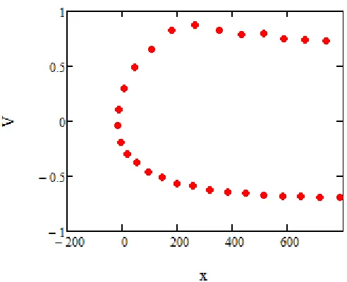
al. There is a range in which, as shown in Figure 2, the averaged velocity decreases along part of the outward trajectory.

∗

Figure 2. The average velocity from the numerical solution fork= 0.6.

Such behaviour can be given by (10), called “uphill acceleration” by Baueret al., if the scaledV is between

1 3k and

1

k,but the average velocity can never cross from the uphill to downhill acceleration regimes in the way that the numerical solution does. In general, if we have any potential quadratic in the electric field, so that the Lagrangian is of the form,

L=1 2mV

2_+F(V)E

0(x)2 (15)

then the equation of motion is

dV dt =−

V F0−F m+F00_E2

0

dE2 0

dx . (16)

With a monotonic intensity profile the acceleration can only change sign if the denominator changes sign, in which case the equation has a singularity, or if the numerator goes through zero. However, using the same argument already given for the Baueret al. formula, the velocity can tend asymptotically to the value at which the numerator goes to zero if the intensity gradient is long enough, but never cross it. Another argument for the impossibility of a Lagrangian with a potential of this form is that the invariant V_∂V∂L −L is of the form

1 2mV

2_{+ (V F}0_−F)E2

0.For a given value ofV this means that there must be a unique value ofE 2

0 , while in our

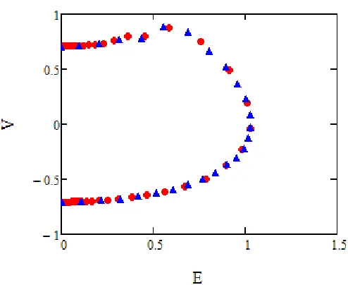
numerical solution the average velocity goes through the same value at different positions with different values ofE02.That there is still an invariant associated with some more complicated form of Lagrangian is suggested

by comparing solutions with exponential and linear intensity dependence (the latter with E0 = 1−₁₀₀₀x for

x <1000, zero otherwise) and plotting the relation betweenE0 andV along the particle orbits, with the result

Figure 3. The relation between the electric field amplitude and the average velocity for the exponential (red circles) and linear (blue triangles) profiles, both withk= 0.6.

3. CONCLUSIONS

We have looked at a very basic problem concerning ponderomotive force, the orbit of a single particle being reflected by an electrostatic wave with a monotonic intensity profile, comparing the numerical solution of the equation of motion with the predictions of averaged Lagrangian theory. While we have concentrated on a particular theory of the ponderomotive force given by Bauer et al., mainly because it gives an explicit formula for the force relevant to our problem, the averaged ponderomotive potential is the same as that quoted by other authors using a variety of methods. Our work shows that for small enough values of the wavenumber the analytic theory and the numerical solution agree well, but that there are parameter ranges where the analytic formula encounters a singularity. In some cases the orbit of a particle goes from a region with acceleration down the wave intensity gradient to one where the acceleration is in the opposite direction. While the analytic theory due to Baueret al. can give such uphill acceleration, we show that it cannot give rise to a transition between downhill and uphill acceleration along a single particle orbit. Indeed, we show that no Lagrangian with an average potential which is quadratic in the electric field amplitude can produce such a transition. This leads us to the conclusion that standard theories must, in some regimes, be extended to include higher order terms in the field amplitude, a problem on which we are currently working. The ponderomotive force is a fundamental idea, widely applied in plasma physics, so we believe that it is of interest to note that even in a very basic configuration there are circumstances in which widely used theoretical models do not apply.

4. APPENDIX: NUMERICAL METHODS

The numerical calculations were carried out using Mathcad 15, but could easily be reproduced on Maple, Mathe-matica or any other matheMathe-matical software with ordinary differential equation solvers. Both Adams and adaptive Runge-Kutta routines were used and shown to give consistent results. In scaled units throughout, the particle was started fromx= 4000 and followed for 104 _{time steps, sufficient to follow the particle through reflection}

ACKNOWLEDGMENTS

This work was supported by the UK Engineering and Physical Sciences Research Council grant EP/N028694/1 “Lab in a bubble” and the UK Science and Technology Facilities Council grant ST/G008248/1. All of the figures were produced using Mathcad 15 on a standard desktop computer, and the data in the figures can be entirely generated using the methods specified in the paper.

REFERENCES

[1] A. A. Vedenov, A . V. Gordeev and L. I. Rudakov, Plasma Phys.9, 719 (1967) [2] J.R. Cary and A.N. Kaufman, Phys. Rev. Lett.39, 402 (1977)

[3] G.W. Kentwell, J. Plasma Phys.34, 289 (1985)