3D Gaze Point Localization and Visualization Using LiDAR-based 3D Reconstructions

Rochester Institute of Technology

RIT Scholar Works

Theses Thesis/Dissertation Collections

12-2015

3D Gaze Point Localization and Visualization

Using LiDAR-based 3D Reconstructions

James Pieszala

[email protected]

Follow this and additional works at:http://scholarworks.rit.edu/theses

Recommended Citation

3D Gaze Point Localization and Visualization Using

LiDAR-based 3D Reconstructions

APPROVED BY

SUPERVISING COMMITTEE:

Dr. Reynold Bailey, Supervisor

Dr. Joe Geigel, Reader

3D Gaze Point Localization and Visualization Using

LiDAR-based 3D Reconstructions

by

James Pieszala, B.S., B.A.

THESIS

Presented to the Faculty of the Golisano College of Computer and

Information Sciences

Rochester Institute of Technology

in Partial Fulfillment

of the Requirements

for the Degree of

Master of Science

in Computer Science

Department of Computer Science

Rochester Institute of Technology

Acknowledgments

This material is based on work supported be the National Science

Foun-dation under Award No. IIS-0952631. Any opinions, findings, and conclusions

or recommendations expressed in this material are those of the author(s) and

do not necessarily reflect the views of the National Science Foundation.

We would like to express appreciation to FARO for donating their

time, equipment and resources; and specifically to account manager Scott

Ger-showitz who preformed all scanning at the West Virginia University’s mock

crime scene facility. We also thank Jacqueline Speir for hosting us at West

Virginia University and assisting in our data collection.

I would personally like to thank Professor Reynold Bailey for his

con-tinual support and faith in this project over the last two years; it was his

research interests that first inspired me to embark on this exploration. Others

to thank: Professor Joe Geigel for extending his resources and time, the RIT

Computer Graphics and Applied Perception Lab for fostering creative insights,

Abstract

3D Gaze Point Localization and Visualization Using

LiDAR-based 3D Reconstructions

James Pieszala, M.S.

Rochester Institute of Technology, 2015

Supervisor: Dr. Reynold Bailey

We present a novel pipeline for localizing a free roaming eye tracker

within a LiDAR-based 3D reconstructed scene with high levels of accuracy. By

utilizing a combination of reconstruction algorithms that leverage the strengths

of global versus local capture methods and user-assisted refinement, we reduce

drift errors associated with Dense Simultaneous Localization and Mapping

(D-SLAM) techniques. Our framework supports region-of-interest (ROI)

an-notation and gaze statistics generation and the ability to visualize gaze in 3D

from an immersive first person or third person perspective. This approach

gives unique insights into viewers’ problem solving and search task strategies

Table of Contents

Acknowledgments iii

Abstract iv

List of Figures vii

Chapter 1. Introduction 1

Chapter 2. Background 5

2.1 SLAM . . . 5

2.2 Requirements . . . 6

2.3 LiDAR . . . 7

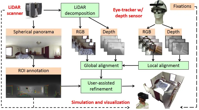
Chapter 3. System Design 9 3.1 Overview . . . 9

3.2 Equipment and Data Collection . . . 10

3.3 Local Alignment . . . 12

3.3.1 2D Feature Projection . . . 13

3.3.2 RANSAC 3-Point Algorithm . . . 15

3.3.3 Local Camera Tracks . . . 17

3.4 Global Alignment . . . 17

3.4.1 LiDAR Decomposition . . . 17

3.4.2 Perspective N Point Algorithm . . . 18

3.5 ROI Annotations . . . 19

3.6 Simulation and Visualization . . . 21

Chapter 4. Results and Discussion 24 4.1 Alignment Accuracy . . . 25

4.2 Statistical Tools . . . 27

Chapter 5. Conclusion 32

5.1 Novelty . . . 32

5.2 Limitations . . . 32

5.2.1 Alignment Range . . . 32

5.2.2 High End LiDAR . . . 33

5.2.3 Scene Complexity . . . 33

Chapter 6. Future Work 35 6.1 Improved Depth Map Accuracy . . . 35

6.2 Improved Global Registration . . . 36

6.3 Addressing LiDAR Based Reconstructions . . . 36

6.4 Improved Dense-SLAM Results . . . 37

Bibliography 38

List of Figures

1.1 Early 3D gaze analysis . . . 2

1.2 Alignment of single frame from an eye-tracker with 3D recon-structed scene . . . 4

3.1 Pipeline overview . . . 10

3.2 Head mounted capture rig setup . . . 11

3.3 Depth to RGB registration . . . 13

3.4 Depth map projection . . . 14

3.5 Estimating a rigid transformation. . . 15

3.6 LiDAR decomposition . . . 18

3.7 Eye tracker offset . . . 19

3.8 LiDAR annotation tool . . . 20

3.9 Utilizing ROI annotations . . . 22

3.10 Hi-Def LiDAR UV texturing . . . 23

4.1 Locally-aligned camera chunks . . . 25

4.2 Point cloud alignment comparison . . . 26

4.3 RGB-D frame to LiDAR error metric . . . 27

4.4 Global alignment error via RANSAC . . . 29

4.5 Global alignment error via RANSAC plus ICP . . . 29

4.6 Gaze collision via ray casting . . . 30

4.7 Breakdown of attended ROIs . . . 30

4.8 Heat map visualizations . . . 31

Chapter 1

Introduction

The field of 3D scanning and geometric reconstruction has been

chang-ing at an unprecedented rate over the past 20 years. The commercialization

of competing 3D data acquisition technologies has served to lower prices and

empower practitioners in many disciplines including medical imaging, cultural

heritage documentation, gaming, craft and remodeling, and 3D printing.

Au-tomated scanning techniques are also increasingly being used to document

crime scenes. These scans are valuable to forensic scientists as they can be

revisited as many times as desired, and by as many experts as needed, over

the course of an investigation.

The ability to localize a head-mounted eye-tracker and visualize the

3D point-of-regard within these reconstructed environments provides valuable

insights into viewers’ problem solving and spatial processing strategies.

How-ever, the existing visualization techniques, developed for remote eye-tracking

systems, are not directly applicable with head mounted eye-trackers. In

re-mote systems, the relationship between the eye-tracker and display on which

the stimuli are presented is fixed, making it straightforward to visualize the

eye-trackers, the viewer can move freely about the 3D environment, hence both

the perspective and stimuli will differ across subjects. Early approaches to

ad-dress this challenge relied on the creation of a panorama using key frames from

one subject’s eye-tracker scene camera video [21]. The gaze points gathered

from all subjects performing the task were then mapped onto this panorama

as shown in Figure 1.1. This work was later extended to map multiple

view-ers’ fixations onto a high-resolution ‘Gigapan’ image captured from a central

location [16]. However such approaches require that viewers observe the scene

from roughly the same vantage point and do not preserve the relative positions

of objects in the scene.

More recently, with the advances in 3D scanning, reconstruction

tech-nologies and computer vision algorithms, more robust techniques for 3D gaze

analysis are beginning to emerge [3, 14, 20]. However, techniques for

localiza-tion of the head and eye-tracker within the 3D scene often still rely on external

motion capture cameras [7] which require considerable setup and calibration

time. The external cameras installations also change the context of scene

which my compromise certain search tasks experiments. These restrictions

often render such systems impractical or unfeasible for many applications.

The pipeline described in this paper enables simulation and

visualiza-tion of gaze data from multiple viewers on a single 3D model of the scene

without the need for an external motion capture system. The subjects are

free to move about the scene which leads to more natural task performance.

Furthermore, since it is not necessary to warp the scene camera video into a

flat panorama, our system preserves the relative positions of the objects in the

scene during the visualization process.

Our pipeline utilizes a combination of global and local 2D and 3D

regis-tration techniques to align the imagery from a head-mounted eye-tracker and a

head-mounted depth camera with depth and RGB data from a high resolution

LiDAR scanner. Our pipeline supports region-of-interest (ROI) annotation

which facilitates the generation of ROI-based gaze statistics. The user-created

ROI annotations are also leveraged to further refine the alignment between the

eye-tracker scene-camera imagery and the LiDAR 3D data. Figure 1.2 shows

two perspectives of one frame of this alignment - a first-person view and a

third-person view. This approach solves the problem of maintaining the 3D

scene context and grants researchers increased insight into subjects’ problem

solving strategies. Visualizations can be created which highlight the regions

of the scene that were attended to (or not attended to) by the subjects.

The remainder of this paper is organized as follows: relevant

Figure 1.2: Alignment of single frame from an eye-tracker with 3D recon-structed scene. (Left) First-person perspective - the blue marker indicates the current fixation point and the 3D model is shown without RGB texturing. (Right) Third-person perspective - showing eye-tracker scene camera pose and corresponding 3D point-of-regard, 3D model is depicted with high resolution LiDAR texturing.

of our pipeline is presented in Chapter 3, results highlighting the capabilities

of our solution are presented in Chapter 4, overall contributions and

limita-tions are discussed in Chapter 5, and the paper concludes in Chapter 6 with

Chapter 2

Background

Our approach is general enough to find a home in many applicable

ar-eas of spatial cognition research; however, it’s main impetus and field of direct

applicability is that of crime scene investigation. CSI generally requires

in-vestigative scenes to remain static and without the introduction of external

equipment such as a motion capture apparatus. Along with these

require-ments, any solution must also have a minimal set up time, as to facilitate ease

of use for practitioners. Our initial approach begins by leveraging recent

ad-vances in 3D reconstruction that utilize RGB-D sensors. While techniques of

this nature are attractive because they require no previous preparation of the

scene, certain inherent limitations have demanded a more elaborate solution.

The following sections aim at highlighting relevant technologies and

method-ologies that have informed our overall approach of localizing and visualizing

3D gaze data.

2.1

SLAM

The challenge of localizing a free roaming head mounted eye tracker

and is closely related to the Simultaneous Localization and Modeling (SLAM)

problem. SLAM arising from the question of whether a sensing entity can

build a map of its surroundings while also locating itself within such a map.

In the last 30 years SLAM based solutions have continually evolved with ever

available technologies and increased processing power. Of late, SLAM

solu-tions continue to benefit from the introduction of relatively inexpensive

RGB-D sensors, such as the Microsoft Kinect. Solutions of this type generally fall

under the category of Dense-SLAM. Microsoft Research’s Kinect Fusion [19]

is credited as being the first Dense-SLAM solution to produce real time

sub-centimeter 3D reconstructions. Since this seminal work of 2011, a wealth of

literature has been published that continue to exploit the capabilities of these

new inexpensive sensors [30]. A common theme of this continual research is

that of addressing concerns of drift error, and limitations of scan size in real

time operations.

2.2

Requirements

Owing to the unpredictable nature inherent in human search task

strate-gies, localizing a head mounted sensor presents a unique set of requirements to

the SLAM paradigm. Foremost in our requirements is that any solution should

not place any restrictions on natural human temporal-spatial movements. Due

to this requirement and its consequences, a strict SLAM only solution will not

entirely suffice as they generally require relatively slow capture movements and

gaps and in some circumstances result in sensor trajectories with zero

correla-tion. In order to resolve the sequences of disparate trajectories some type of

a global map is required.

We propose that by augmenting a SLAM based solution with a certain

number of LiDAR scans, limitations of a SLAM-only solution can be addressed,

while at the same time, improving SLAM accuracy for when it is required. In

order to maintain a reasonable set up time for practitioners, we aim to use

the least number of LiDAR scans as possible. Here a balance must be struck

between allowing SLAM to gather model data in complex scenes (occluded

in a LiDAR scan), and having fair LiDAR coverage to keep SLAM localized

and accurate. As we envision this framework would be applied to scenes

constructed in the interest of spatial cognition research, it is reasonable to

expect that these balances can be controlled to ensure complete eye tracker

alignment. For on-the-fly real world scenarios, a more formal criteria will need

to be in place for determining the optimal number of LiDAR scans needed

[27]. The data used in this thesis has come from a mock crime scene; which is

well suited for this approach’s applicable context.

2.3

LiDAR

LiDAR based scanners are increasingly being used to document crime

scenes. Their ability to document a scene as a highly accurate 3D

reconstruc-tion has many addireconstruc-tional benefits over tradireconstruc-tional photographic

real world geometry; which, for example, is extremely useful in blood spatter

and ballistics analysis. Owing to LiDAR’s continual rise as a CSI tool, we see

this as additional evidence of the feasibility of its use in our pipeline.

The nature by which a LiDAR scanner, like a FARO Focus3D captures

data, makes it ideally suited for tracking a roaming RGB-D sensor. It provides

a highly accurate spherical RGB-D data that the roaming sensor can operate

Chapter 3

System Design

3.1

Overview

Our goal is to incorporate recent advances in Dense-SLAM based 3D

reconstruction with the global accuracy of LiDAR point clouds to facilitate

the localization of head mounted eye trackers and associated 3D

points-of-regard. To accomplish this, we seek to balance the disadvantages of some

stand-alone solutions with the advantages of others. For instance, low-cost

RGB-D capture devices such as the Microsoft Kinect provide ease of use and

mobility but often suffer from noisy alignments and global drifting; on the

other hand, LiDAR based scanners produce highly accurate global 3D point

clouds but are often restricted to rigid anchor points. Recent innovations

in Dense-SLAM reconstructions [5, 29, 31] have mitigated drift and erroneous

alignments to varying degrees, and our strategy proceeds by leveraging these

existing solutions and augmenting them with LiDAR tie points. This technique

will ultimately allow us to extend the many benefits of a Dense-SLAM solution

to handle the added difficulty of tracking unpredictable sensor movements. As

it is generally impractical to have a complete LiDAR scene representation,

Dense-SLAM will ensure that all viewed scene geometry will be accounted

Figure 3.1: System overview and data flow.

to validate and refine the alignment between the eye-tracker scene camera

imagery and the LiDAR 3D data. This approach produces high accuracy

camera frame alignments with correspondingly high quality 3D models that

can be used in the research of 3D gaze behavior. Figure 3.1 provides an

overview of our system and illustrates the general flow of information through

our pipeline.

3.2

Equipment and Data Collection

The data used in this paper to demonstrate the capabilities of our

pipeline were collected at a crime scene training facility at West Virginia

Figure 3.2: Head mounted capture rig: an SMI eye tracker with a rigidly positioned RGB-D sensor.

FARO Focus3D laser scanner. A typical indoor scan consists of 10.8 million

data points with millimeter accuracy. In addition, each scan also captures a

high resolution spherical panorama which we later use for global alignment,

texture mapping and ROI annotation.

For eye-tracking, we used a SensoMotoric Instruments Eye Tracking

Glasses (ETG) with a 1280 x 960 scene camera operating at 24 fps and 640

x 480 binocular eye-cameras operating at 60 fps. A PrimeSense Carmine

depth sensor was fixed to the head of the viewer in close proximity to the

SMI eye-tracker. The PrimeSense sensor is equipped with 640 x 480 RGB

and depth cameras operating at 30 fps. Experiments were also conducted

using a Microsoft Kinect sensor. While not an elegant solution, this approach

facilitates higher accuracy alignments and the depth information from the

PrimeSense sensor is used to fill gaps in the LiDAR data. Future head-mounted

approach. Members of our research team took turns walking through the crime

scene facility using this system to collect pilot data.

3.3

Local Alignment

Local alignment refers to the serial alignment of consecutive camera

frames from the same device. Local alignment is performed on the RGB-D

video feed from the head-mounted sensor. We urge the reader to note that

following alignment techniques pertain only to the RGB-D sensor. The actual

eye tracker location is calculated relative to the RGB-D sensor as the last stage

of the pipeline before final simulation and visualization.

Each RGB frame is first processed using a wavelet based blur detector.

If a frame exhibits significant blur due to rapid head movement, it is flagged

and ignored in order to mitigate local alignment errors. In the event that

an entire fixation is lost due to blurry frames, the least blurry flagged frame

(within a fixation) can be reintroduced and aligned with manual input during

the final refinement stage. We have found this approach to be reasonable for

relatively deliberate tasks, such as crime scene examinations.

Once the blurriest frames have been removed, the remaining camera

frames are fed into a Dense-SLAM alignment algorithm. Our approach is

adapted from Xiao et al.[31]. We use their SIFT feature-based serial alignment

technique where corresponding depth coordinates are fed into a RANSAC

3-point-algorithm which solves for relative camera pose. This SIFT based

because it is able to align frames over larger distances. Additional fine tuning

is done with ICP and generalized bundle adjustment. In our implementation,

we omit their loop closure module since the corresponding LiDAR associations

make it mostly unnecessary. The reason for performing these local alignments

first is that if a subsequent LiDAR alignment fails, the relative local

associ-ations will have already been computed and maintained. The following two

sections delve deeper into the alignment algorithm for consecutive RGB-D

frames.

3.3.1 2D Feature Projection

RGB-D sensor recordings were performed using the OpenNI software

suite. We have also utilized OpenNI’s built in support for depth-to-RGB

frame registration in order merge both sets of data into the same RGB camera

coordinate system. Figure 3.3 shows one such registration. Note how the

depth image has been adjusted. Subsequent projection calculations can now

Figure 3.3: Depth to RGB registration. (Left) A depth frame automatically aligned to its (Right) RGB frame.

general 3D to 2D projection using the RGB camera intrinsic matrix retrieved

by OpenNI; where,fx, andfy are the focal lengths in pixels, andcx andcy are

principal point offsets. By inverting this transformation, equations 3.2 and 3.3

can be used to back project the 2D depth map into 3D. This same approach

is used to obtain the corresponding 3D point of any 2D SIFT features that

have been detected. Figure 3.4 shows a simplified visualization of this back

projection process.   x y 1  =  

fx 0 cx

0 fy cy

0 0 1

    X Y Z   (3.1)

X= (x−cx)(Z/fx) (3.2)

Y = (Y −cy)(Z/fy) (3.3)

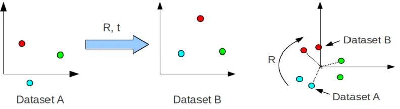
3.3.2 RANSAC 3-Point Algorithm

The 3 point algorithm is a solution for estimating the rigid

transfor-mation between successive pairs of camera poses [8, 12]. Input points into

the algorithm are the projected depth map points that directly correspond to

the 2D SIFT matches. Below is the algorithmic flow for estimating a rigid

transform from points Pa to Pb. First, centroids of each set of 3D points are

computed. Relative point offsets from these centroid origins are then found

for each point set and multiplied against each other to form matrix H. Single

Value Decomposition solves for the rotational component of the rigid

trans-form, and the translation component arises from applying this rotation to one

centroid origin and computing the shift from the other.

B =R∗A+t

P = [x, y, z]T

centroidA=

1

N

N

X

i=1

P_Ai

centroidB=

1

N

N

X

i=1

P_Bi

H=

N

X

i=1

(P_Ai −centroidA_)(Pi

B−centroidB)

[U, S, V] =SV D(H)

R=U VT

t=−R∗centroidA+centroidB

In order to detect and eliminate outliers, RANSAC is used with the 3

point algorithm being its fitting function. The algorithm proceeds as follows:

(1) randomly sample 2D SIFT point pairs between the frames in question,

(2) Fit the model using the fitting function (3-Point Algorithm), (3) check

all original points pairs fitting this model and form a consensus, (4) refit the

model on all consensus points, and lastly (5) repeat on consensus points if we

are still above the error threshold, or reject model and start with a fresh set

of random point pairs. The algorithm will succeed and stop once consensus

points fitting the model are within a predetermined error range. Otherwise, if

3.3.3 Local Camera Tracks

Due to any large and rapid head movements that may have been present,

local sequential alignment may produce a number of disparate camera tracks

that are uncorrelated. The next section shows how a global map solves this

issue.

3.4

Global Alignment

Global alignment refers to aligning the frames from a head mounted

RGB-D sensor with the LiDAR 3D data. As a first step we prep the LiDAR

data to be in a comparable format as our roaming RGB-D frames, in what

we refer to as LiDAR Decomposition. Once in this format, we can perform

planar 2D feature matching techniques with the locally aligned frames. In

the following section we detail this process along with the final step of solving

for the offset between the eye-tracker and head-mounted depth sensor using a

general perspective-n-point algorithm.

3.4.1 LiDAR Decomposition

Since the LiDAR scanner uses spherical data acquisition, we project the

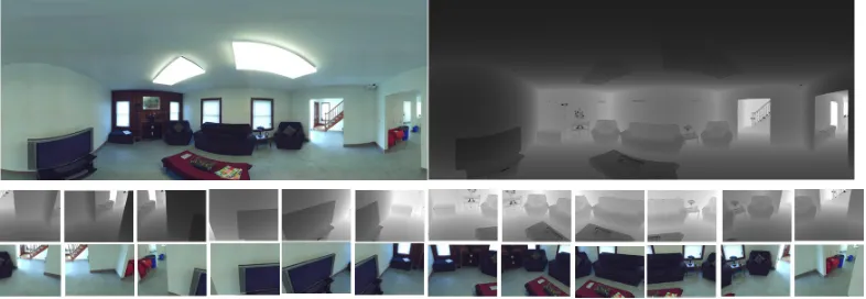
RGB and depth data onto 640 x 480 virtual planar frames, similar to Zhang

et al. [32]. Figure 3.6 shows this decomposition for one horizontal sweep. To

increase possible matching perspectives we use a %50 overlap for the LiDAR

frames. To further increase matching perspectives, this technique is easily

Figure 3.6: LiDAR Decomposition: 12 planar frames used in global alignment

The global alignment process follows a similar methodology as the local

alignment procedure described above. We perform brute force matching of

each decomposed LiDAR frame against each roaming frame using a modified

version of the Xiao et al. algorithm [31], discussed above. The LiDAR frame

that produces the highest number of successful inliers will be used to align the

roaming RGB-D. Frames that do not globally register are adjusted relative

to their closest globally aligned neighboring frame. If necessary, additional

bundle adjustment can be done to further reduce alignment errors.

3.4.2 Perspective N Point Algorithm

In order to calculate the eye tracker offset relative to the RGB-D

sen-sor we use 3D to 2D point correspondences. First, 2D matching SIFT

fea-tures are found between eye tracker frames and RGB-D sensor frames that

share the same time stamp. Figure 3.7 shows the relative alignment of the

Figure 3.7: SIFT matching between eye tracker and RGB-D sensor. (Left) Relative camera placement in capture rig. (Middle) RGB frame of depth sensor. (Right) Eye tracker frame.

pair. Using the depth data from the RGB-D SIFT matches we are supplied

with 3D to 2D points correspondences for the eye tracker. In general, for

the computation of a camera pose matrix the minimal solution requires 6

point correspondences. These correspondences can be fed into a direct linear

transformation algorithm. In cases where certain assumptions can be made,

a restricted camera estimation can be performed [9]. Specifically, if the

cam-era calibration matrix is known before hand, certain algorithms can compute

the pose matrix with as few as 3 point correspondences. Such algorithms

in-clude variants on Levenberg-Marquardt minimization. Throughout my test

cases I’ve used OpenCV’s routine SolvePnP which is based on an iterative

Levenberg-Marquardt implementation.

3.5

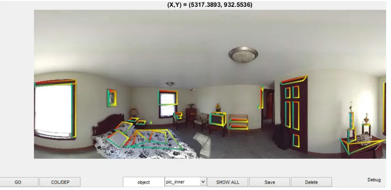
ROI Annotations

Typically in eye-tracking experiments, task-relevant objects or regions

in the reporting of gaze statistics. In our pipeline, the user-created ROIs are

also utilized to verify the accuracy of the recovered scene-camera alignments.

Figure 3.8 shows our Matlab based LiDAR annotation tool. Regions are

man-ually chosen by clicking out boundary boxes, and the underlying 3D points

are then saved out in appropriate data structures.

Figure 3.8: LiDAR annotation tool

After the alignment stages have been completed a second Matlab based

user interface is used for refinement and validation. This is accomplished

by projecting the 3D LiDAR ROIs (previously recorded), onto the localized

camera frames. Once this is done, misaligned regions are easily noticed and can

be manually adjusted. Figure 3.9 (Bottom) displays this second Matlab based

GUI. Notice that as with the previous interface, the depth map can also be

used to assist in this process. Any adjustments will result in a camera matrix

further ROI annotations for regions that may not have been available in the

LiDAR data.

3.6

Simulation and Visualization

The finalized camera frame parameters, ROI annotations, eye-tracker

event data, and relevant 3D models are sent to a simulation and visualization

application. This application constructs virtual camera models corresponding

to the recovered camera parameters and projects 2D gaze events onto the 3D

scene model. The application is built using the Unity3D framework, and

al-lows for a variety of interactive options including first-person and third-person

playback perspectives, 3D heat map generation, active ROI visualization, and

3D gaze statistics generation. Using the registered RGB data from the FARO

LiDAR scanner, we can easily apply high resolution texturing to the scene.

For real-time interaction and rendering, the high resolution textures can be

applied to decimated meshes and still maintain visual detail, as seen in

Fig-ure 3.10. Our visualization system is fully operable as a VR solution with

Chapter 4

Results and Discussion

As expected, camera tracks at slower speeds exhibited the highest

au-tomated local alignment accuracy due to less motion blur. Currently our

wavelet-based blur detector uses a manually set conservative threshold to flag

blurry frames. Using this approach across all of our data sets we observe a

worst-case of 36% of frames being flagged. We found this threshold to be good

compromise between maintaining fixation data integrity and labor necessary

for manual refinement. As the threshold is increased to allow more frames to

pass through, greater effort may be required in the refinement stage if no global

align exists. The occurrence of blurry frames drops off significantly when the

viewer is engaged in deliberate visual scanning of the scene. We envision using

more elaborate threshold optimization techniques and higher-speed cameras

to improve local alignment percentages.

Figure 4.1 illustrates the five longest locally aligned camera tracks from

the head-mounted depth sensor. This particular data set was the worst in

terms of the number of blurry frames. Figure 4.2 (Top) shows the

correspond-ing local and global alignments. Notice that there is little correspondence

align-Figure 4.1: Locally-aligned camera path groups from the head-mounted depth sensor shown in different colors.

ment step is able to resolve this (Top right). For comparison, the bottom

images show the local and global alignments from a deliberate visual scan

(best-case).

4.1

Alignment Accuracy

Alignment error metrics are achieved by comparing 2D pixel distances

between matched features used in the global alignment stage. The underlying

3D points associated with 2D LiDAR features are projected onto the newly

aligned roaming frame and compared against their matched 2D roaming frame

features. Figure 4.3 displays the 2D SIFT features used to align one such

roaming frame. The red toruses show the corresponding 3D LiDAR features

that have been projected onto this newly aligned frame. By taking the average

Figure 4.2: Alignment Comparison. (Top) Local and global alignments from our worst-case (most rapid visual scan of the scene). (Top left) Local alignment showing five main continuous frame groups. (Top right) Corresponding depth cloud after global alignment with LiDAR model. (Bottom) Local and global alignments from a deliberate visual scan (best-case).

for frame alignment accuracy. Figure 4.4 shows the global alignment results for

all 2016 frames contained in the kitchen dataset. Figure 4.5 shows the results of

this same error analysis technique after the additional step of iterative closest

point (ICP) fine tuning. As can be observed, ICP increases the effective gaze

projection error from 0.5 angular degrees in the RANSAC-only case to 0.65

degrees. The fact that the ICP algorithm is actually producing an increase in

average alignment error is a direct consequence of the roaming depth sensor’s

Figure 4.3: Frame Alignment Accuracy. (Right) A roaming frame being glob-ally aligned. SIFT features in Blue, corresponding LiDAR features in red. (Left) The decomposed LiDAR frame used in alignment. SIFT features dis-played in red.

and depth map de-noising, our method could achieve pixel accuracy projection

(0.1 degrees).

4.2

Statistical Tools

The effective output our pipeline and main statistical resource is the

list of 3D points-of-regard. 3D points-of-regard are computed by ray casting

the gaze vector for each aligned eye-tracker frame by way of appropriately

constructed pinhole camera models. Collision detection is computed against

the 3D scene reconstruction and recorded accordingly. Additional outputs

include time stamps for each collision along with which, if any, ROI that has

been attended to. Figure 4.7 displays a basic histogram of the relative time

4.3

Additional Tools

We have developed a technique to present 3D gaze information in a 2D

panoramic format. This facilitates the reporting and analysis of gaze behavior

for certain scene contexts; specifically, those that are able rely solely on

gaze-to-LiDAR statistics. A 2D heat map is computed based on a conical search

initiated from a depth dependent radius at the 3D point-of-regard that affects

only the corresponding 2D projected pixels. Figure 4.8 (Bottom) shows an

Figure 4.4: Global alignment error via RANSAC for the kitchen dataset. Average pixel and angular error per globally aligned frame.

Figure 4.6: Gaze collision via ray casting. The red upper shelf shows an ROI collision has occurred.

Chapter 5

Conclusion

By augmenting Dense SLAM-based reconstruction techniques with the

global accuracy of LiDAR clouds, our results have shown a feasible solution

to eye-tracker localization and accurate 3D point-of-regard recovery for indoor

static scenes. We believe our solution supplies a much needed tool in order to

fully exploit and research data obtained from head-mounted eye-trackers.

5.1

Novelty

Our solution’s novelty arises from applying a unique combination of

existing computer vision techniques to address the new and challenging

prob-lem of how to extract complete 3D gaze data from head mounted eye trackers.

We believe that by utilizing our framework, new experiments in 3D spatial

cognition and processing will now be possible.

5.2

Limitations

5.2.1 Alignment Range

Our technique is indeed more applicable to certain eye-tracking

strategies placing the viewer within the proper depth sensor range;

gener-ally, between 0.4 meters to 4 meters of scene geometry. For our main design

context, this is generally not an issue as we target search tasks requiring

de-liberate examination of objects (such as crime scene investigation); which,

typically fall within this range.

5.2.2 High End LiDAR

We argue that a global map is needed to effectively localize an eye

tracker subject to natural head movements. And while this can be

accom-plished using external motion capture devices, such approaches are often not

feasible due to significant setup time and the need for several synchronized

cameras. Placing these cameras in the scene also changes the content of the

scene which may compromise the task at hand. The alternative is to rely on

3D scans of the environment which is the approach we employ. Due to cost, the

ability to obtain a high end LiDAR scanner may be seen as a limiting factor.

However, the reader should note that LiDAR costs are similar to that of head

mounted eye trackers, and are continuing to fall in price. And, although our

system can be used with lower quality scanners, as with all computer vision

techniques, better quality input leads to better quality results.

5.2.3 Scene Complexity

Complexity of a scene will dictate results. As scene complexity

scans, or (2) relay more on local SLAM results. How this choice dictates

final results is highly dependent on the eye tracking task being performed.

For example, if complex scene geometry is combined with a task expecting

rapid and large head movements, then more LiDAR scans will be needed to

retain high levels of automatic global alignment. On the other hand, even

in highly complex scenes, if slower or smaller head movements are expected,

extra LiDAR scans will not be a necessity as Dense-SLAM techniques should

maintain tracking. In the event of no overlap between local and global data,

we can rely on manual alignment or utilize existing methods to automatically

identify additional locations where the LiDAR scanner can be positioned to

provide additional data [27].

As our technique is primarily a tool for researchers of 3D gaze behavior,

we believe our solution leaves researchers a sufficient context to perform many

meaningful experiments. Specifically, for those researchers who are able to

control their scene contexts, it is possible to design experiments that could

achieve full global alignment.

As pertaining to a plug-and-play tool for crime scene investigation,

LiDAR is increasingly being used to document crime scenes, and LiDAR

tech-nicians are trained to capture the scene with optimal placement and with as

Chapter 6

Future Work

We look forward to putting our solution into practice within an

ap-propriate research study; which, inevitably would supply us with necessary

feedback for future improvements. The following sections detail our present

areas of focus for improved applicability.

6.1

Improved Depth Map Accuracy

First and foremost, a robust RGB-D sensor calibration is needed [13].

The present rudimentary intrinsic matrix consisting of focal lengths and

princi-pal offset points is seen as the main road block to achieving the highest possible

3D point-of-regard accuracy. Further work is also needed to improve the

ac-curacy of individual depth frame maps. A depth map can be denoised [31]

by accumulating neighboring depth frames into a voxel grid and re-sampling

from the depth map’s perspective. We believe that once these improvements

6.2

Improved Global Registration

As alluded to in the introduction, a formal study will need to be done

to find the optimal number of LiDAR scans required. Metrics will need to

be formulated to address scene complexity and extent of local drift expected

when LiDAR scan data is not present. Also, for higher probabilities of global

registration we could increase the number of LiDAR frames used in the

decom-position stage. We presently have restricted our pipeline to 12 decomposed

LiDAR frames mainly due to the inefficiency of the brute force global matching

algorithm. By instead setting an acceptable error threshold for registration,

we can stop checking all possible LiDAR frames when this threshold is reached

and then start matching the subsequent frame at this location. Another option

for increased global registration would be to explore and implement additional

registration techniques, such as 3D feature matching.

6.3

Addressing LiDAR Based Reconstructions

We are presently working on a solution to automatically use data from

the head-mounted depth sensor to fill gaps in the LiDAR data. This will be

invaluable for additional ROI annotation, complete 3D point-of-regard

statis-tical analysis, and better visualization coverage. Figure 6.1 shows some results

of this present work. Visualization concerns will need to be addressed as issues

will arise when choosing between the LiDAR’s seamless texturing, and meshes

captured with alternate lighting perspectives. Whichever final model solution

Figure 6.1: Model Merging. (Left) LiDAR model, (Middle) Roaming depth mesh from one frames perspective, (Right) Merged result

real time simulations [24].

6.4

Improved Dense-SLAM Results

Our work thus far has focused mainly on how LiDAR global maps can

extend the applicability of a Dense-SLAM solution to a head mounted sensor.

We propose that the LiDAR data can also improve local alignment accuracy,

Bibliography

[1] Sameer Agarwal and Keir Mierle. Ceres solver: Tutorial & reference.

Google Inc, 4, 2012.

[2] C. Antonya. Accuracy of gaze point estimation in immersive 3d

inter-action interface based on eye tracking. In Control Automation Robotics

Vision (ICARCV), 2012 12th International Conference on, pages 1125–

1129, Dec 2012.

[3] Thomas Booth, Srinivas Sridharan, Vasudev Bethamcherla, and Reynold

Bailey. Gaze3d: Framework for gaze analysis on 3d reconstructed scenes.

In Proceedings of the ACM Symposium on Applied Perception, SAP ’14,

pages 67–70, New York, NY, USA, 2014. ACM.

[4] Jiawen Chen, Dennis Bautembach, and Shahram Izadi. Scalable

real-time volumetric surface reconstruction. ACM Transactions on Graphics

(TOG), 32(4):113, 2013.

[5] Sungjoon Choi, Qian-Yi Zhou, and Vladlen Koltun. Robust

reconstruc-tion of indoor scenes. In Proceedings of the IEEE Conference on

Com-puter Vision and Pattern Recognition, pages 5556–5565, 2015.

[6] Gabriel Diaz, Joseph Cooper, Dmitry Kit, and Mary Hayhoe. Real-time

environment. Journal of vision, (12):1–14, January 2013.

[7] Kai Essig, Daniel Dornbusch, Daniel Prinzhorn, Helge Ritter, Jonathan

Maycock, and Thomas Schack. Automatic analysis of 3d gaze

coordi-nates on scene objects using data from eye-tracking and motion-capture

systems. InProceedings of the Symposium on Eye Tracking Research and

Applications, pages 37–44. ACM, 2012.

[8] David A Forsyth and Jean Ponce. A modern approach. Computer

Vision: A Modern Approach, 2003.

[9] R. I. Hartley and A. Zisserman. Multiple View Geometry in Computer

Vision. Cambridge University Press, ISBN: 0521540518, second edition,

2004.

[10] Richard I Hartley. Estimation of relative camera positions for

uncali-brated cameras. InComputer VisionECCV’92, pages 579–587. Springer,

1992.

[11] Peter Henry, Michael Krainin, Evan Herbst, Xiaofeng Ren, and Dieter

Fox. Rgb-d mapping: Using depth cameras for dense 3d modeling of

indoor environments. InIn the 12th International Symposium on

Exper-imental Robotics (ISER. Citeseer, 2010.

[12] Nghia Ho. Finding optimal rotation and translation between

[13] Kourosh Khoshelham and Sander Oude Elberink. Accuracy and

reso-lution of kinect depth data for indoor mapping applications. Sensors,

12(2):1437–1454, 2012.

[14] Morten Lidegaard, Dan Witzner Hansen, and Norbert Kr¨uger. Head

mounted device for point-of-gaze estimation in three dimensions. In

Pro-ceedings of the Symposium on Eye Tracking Research and Applications,

ETRA ’14, pages 83–86, New York, NY, USA, 2014. ACM.

[15] Michael Maurus, Jan Hendrik Hammer, and J¨urgen Beyerer. Realistic

heatmap visualization for interactive analysis of 3d gaze data. In

Pro-ceedings of the Symposium on Eye Tracking Research and Applications,

pages 295–298. ACM, 2014.

[16] Brandon. May. Imaging methods for understanding and improving

vi-sual training in the geosciences. Master’s thesis, Rochester Institute of

Technology, 2013.

[17] Susan M Munn and Jeff B Pelz. 3d point-of-regard, position and head

orientation from a portable monocular video-based eye tracker. In

Pro-ceedings of the 2008 symposium on Eye tracking research & applications,

pages 181–188. ACM, 2008.

[18] Richard A Newcombe and Andrew J Davison. Live dense reconstruction

with a single moving camera. In Computer Vision and Pattern

[19] Richard A Newcombe, Shahram Izadi, Otmar Hilliges, David Molyneaux,

David Kim, Andrew J Davison, Pushmeet Kohi, Jamie Shotton, Steve

Hodges, and Andrew Fitzgibbon. Kinectfusion: Real-time dense surface

mapping and tracking. In Mixed and augmented reality (ISMAR), 2011

10th IEEE international symposium on, pages 127–136. IEEE, 2011.

[20] Lucas Paletta, Katrin Santner, Gerald Fritz, Albert Hofmann, Gerald

Lodron, Georg Thallinger, and Heinz Mayer. Facts-a computer vision

system for 3d recovery and semantic mapping of human factors. In

Computer Vision Systems, pages 62–72. Springer, 2013.

[21] J. Pelz, T. Kinsman, and K. Evans. Analyzing complex gaze behavior

in the natural world. SPIE-IS&T Human Vision and Electronic Imaging

XVI, pages 1–11, 2011.

[22] Thies Pfeiffer. Measuring and visualizing attention in space with 3d

attention volumes. In Proceedings of the Symposium on Eye Tracking

Research and Applications, pages 29–36. ACM, 2012.

[23] Thies Pfeiffer, Marc Erich Latoschik, and Ipke Wachsmuth. Evaluation

of binocular eye trackers and algorithms for 3d gaze interaction in virtual

reality environments. JVRB-Journal of Virtual Reality and Broadcasting,

5(16), 2008.

[24] Thies Pfeiffer, Cem Memili, Patrick Renner, Thies Pfeiffer, Sven Wachsmuth,

Stellmach, et al. Gpu-accelerated attention map generation for dynamic

3d scenes. Journal of Pragmatics, 8684:90–109, 2015.

[25] Fiora Pirri, Matia Pizzoli, and Alessandro Rudi. A general method for

the point of regard estimation in 3d space. In Computer Vision and

Pattern Recognition (CVPR), 2011 IEEE Conference on, pages 921–928.

IEEE, 2011.

[26] Vivek Pradeep, Christoph Rhemann, Shahram Izadi, Christopher Zach,

Michael Bleyer, and Steven Bathiche. Monofusion: Real-time 3d

re-construction of small scenes with a single web camera. In Mixed and

Augmented Reality (ISMAR), 2013 IEEE International Symposium on,

pages 83–88. IEEE, 2013.

[27] Katie N Salvaggio and Carl Salvaggio. Automated identification of voids

in three-dimensional point clouds. In SPIE Optical Engineering+

Ap-plications, pages 88660H–88660H. International Society for Optics and

Photonics, 2013.

[28] Sensormotoric. Smi eye tracker and gaze tracking, 2014.

[29] Thomas Whelan, Michael Kaess, Maurice Fallon, Hordur Johannsson,

John Leonard, and John McDonald. Kintinuous: Spatially extended

kinectfusion. 2012.

[30] Thomas J Whelan. Real-time Dense Simultaneous Localisation and

Ireland Maynooth, 2014.

[31] Jianxiong Xiao, Andrew Owens, and Antonio Torralba. Sun3d: A

database of big spaces reconstructed using sfm and object labels. In

Computer Vision (ICCV), 2013 IEEE International Conference on, pages

1625–1632. IEEE, 2013.

[32] Yinda Zhang, Shuran Song, Ping Tan, and Jianxiong Xiao. Panocontext:

A whole-room 3d context model for panoramic scene understanding. In

Vita

James Pieszala was born in Buffalo, New York on October 30th, 1981,

the son of Kevin and Kathleen Pieszala. He received the Bachelor of Science

degree in Electrical Engineering and the Bachelor of Arts degree in

Mathemat-ics from the State University of New York at Buffalo, in 2005. He is currently

pursuing his Master of Science degree from Rochester Institute of Technology,

United States of America. His research interest includes Graphics,

Visualiza-tion, Rendering, and Computer Vision.

Permanent address: 12483 Clinton St

Alden, New York 14004

This thesis was typeset with LA_TEX† _{by the author.}

†_LA_{TEX is a document preparation system developed by Leslie Lamport as a special}