Internal rationality, learning and imperfect information

City, University of London Institutional Repository

Citation

:

This is the published version of the paper.

This version of the publication may differ from the final published

version.

Permanent repository link:

Link to published version

:

Copyright and reuse:

City Research Online aims to make research

outputs of City, University of London available to a wider audience.

Copyright and Moral Rights remain with the author(s) and/or copyright

holders. URLs from City Research Online may be freely distributed and

linked to.

Discussion Papers in Economics

DP 08/17

School of Economics

University of Surrey

Guildford

Surrey GU2 7XH, UK

Telephone +44 (0)1483 689380

Facsimile +44 (0)1483 689548

Web

www.surrey.ac.uk/economics

ISSN: 1749-5075

I

NTERNAL

R

ATIONALITY

,

L

EARNING AND

I

MPERFECT

I

NFORMATION

By

Szabolcs Deák,

(University of Surrey)

Paul Levine,

(University of Surrey)

Joseph Pearlman,

(City University)

&

Bo Yang

(Swansea University,)

Internal Rationality, Learning and Imperfect

Information

Szabolcs De´ak, Paul Levine†, Joseph Pearlman‡, Bo Yang§

December 1, 2017

Abstract

We construct, estimate and explore the monetary policy consequences of a New Key-nesian (NK) behavioural model with bounded-rationality and heterogeneous agents. We radically depart from most existing models of this genre in our treatment of bounded ratio-nality and learning. Instead of the usual Euler learning approach, we assume that agents are internally rational (IR) given their beliefs of aggregate states and prices. The model is inhabited by fully rational (RE) and IR agents where the latter use simple heuristic rules to forecast aggregate variables exogenous to their micro-environment. We find that IR re-sults in an NK model with more persistence and a smaller policy space for rule parameters that induce stability and determinacy. In the most general form of the model, agents learn from their forecasting errors by observing and comparing them with those under RE making the composition of the two types endogenous. In a Bayesian estimation with fixed propor-tions of RE and IR agents and a general heuristic forecasting rule we find that a pure IR model fits the data better than the pure RE case. However, the latter with imperfect rather than the standard perfect information assumption outperforms IR (easily) and RE-IR com-posites (slightly), but second moment comparisons suggest that the RE-IR composite can match data better. Our findings suggest that Kalman-filtering learning with RE can match bounded-rationality in matching persistence seen in the data.

JEL Classification: E03, E12, E32.

Keywords: New Keynesian Behavioural Model, Internal Rationality, Heterogeneous Ex-pectations, Reinforcement Learning, Imperfect Information

∗

Previous versions of this paper were presented at the CEF 2015 Conference, Taiwan, June 2015; seminars at the Universities of Surrey and Leicester; workshops at the Bank of England, March 2015 and the Tinbergen Institute, October, 2015; a keynote lecture for the third annual workshop of the Birkbeck Centre for Applied Macroeconomics, Birkbeck College, May 20, 2016 and at a end-of-ESRC-project Conference at the University of Surrey, 25-26 January, 2017. Comments from participants are gratefully acknowledged, particularly from discussants Cars Hommes and Domenico Massaro. We acknowledge financial support from the ESRC, grant reference ES/K005154/1.

†

University of Surrey, UK; De´ak: [email protected]; Levine: [email protected] ‡

City University London, UK; [email protected] §

Contents

1 Introduction 1

2 The Standard NK Behavioural Model 3

2.1 The Workhorse NK Model . . . 3

2.2 The Brock-Hommes Behavioural NK Model . . . 4

3 The Non-Linear New Keynesian Model 5 3.1 Households . . . 5

3.2 Firms . . . 7

3.3 Closing the Model . . . 9

3.4 Recovering the NK Workhorse Model . . . 9

4 Perfect versus Imperfect Information 11 5 Internal Rationality 13 6 Stability Analysis 15 7 Heterogeneous Expectations across Households and Firms 15 7.1 Exogenous Proportions of RE and IR Agents . . . 17

7.2 Endogenous Proportions of RE and IR Agents . . . 18

7.3 Wealth Distribution . . . 19

8 Bayesian Estimation 20 8.1 The Measurement Equations and Priors . . . 21

8.2 Identification Checks and Estimation of the Posterior Distribution . . . 22

8.3 Bayes Factor Comparison . . . 24

8.4 Parameter Estimation Results . . . 25

9 Matching Second Moments 26 10 Posterior Impulse Responses and Endogenous Persistence 29 11 Conclusions 31 A Summary of Composite RE-IR Model 35 B Balanced Growth Steady State 40 C Proof of Lemma 42 C.1 Proof of Equation 29 . . . 43

D Addition to Section 7 44

F Solution of Linearized Models under Imperfect Information 47

F.1 Perfect Information Case . . . 50

1

Introduction

This paper constructs, estimates and explores the monetary policy consequences of a New

Keynesian (NK) behavioural model with bounded-rationality and heterogeneous agents. It departs from existing models of this genre in its approach to bounded rationality and learning.

There are broadly two choices made by the learning literature at this point: Euler learning or internal rationality. The first, Euler learning (EL), follows the pioneering work of Evans and Honkapohja (2001) and assumes, in the case of households, that agents forecast their own

consumption decision next period. Furthermore they know the minimum state variable (MSV) form of the equilibrium (equivalent to the saddle-path under rational expectations) and use direct observations or VAR estimates of these states to update their estimates each period

using a discounted least-squares estimator. Then a statistical learning equilibrium is one where this perceived law of motion and the actual one coincide. For firms the same applies except the

decision is on prices made by firms who are no longer locked into a contract.

Although this form of bounded rationality responds to what many regard as an extreme assumption of model-consistent expectations, the departure is only a modest one in that agents

still need to know the MSV form of the equilibrium. The defining characteristic of behavioural macro-models is to limit the cognitive skills of at least a group of agents in the model and this

is achieved by introducing simple ‘heuristic’ learning rules. However this raises the opposite concern regarding the bounds on bounded rationality: with heuristic rules agents may fall considerably short of building rational expectations and such models are particularly vulnerable

to the Lucas critique when policy scenarios are studied. The problem is that agents can depart from rationality in an infinite number of ways leading into the ‘wilderness’ of Sims (1980).

In response to the wilderness concern, the literature on behavioural models adopts a basic general framework pioneered by Brock and Hommes (1997). To limit the departure from ra-tionality and rule out stupid behaviour the approach of reinforcement learning proposes that,

although adaptation can be slow and there can be a random component of choice, the higher the ‘payoff’ (defined appropriately) from taking an action in the past, the more likely it will be taken in the future.1

The alternative approach to learning adopted in this paper assumes that agents are

inter-nally rational (IR) given their beliefs of aggregate states and prices which are exogenous to

their decisions.2 As with the Euler equation approach, agents cannot form model-consistent expectations and instead learn about these variables using their knowledge of the MSV form of the equilibrium. The two approaches then differ with respect to what agents learn about

-their own decisions in the first approach, and variables exogenous to the agents in the second

1_{See Young (2004) for a general treatment of this approach.} 2

approach.3

Proceeding to the linearization about a deterministic steady state, as is usual in the

litera-ture, we show that if we require non-rational agents in the model to forecast only macro-variables exogenous to their decision rules, EL of Evans and Honkapohja (2001) then makes two implicit assumptions: agents (1) know they are all identical and (2) observe the state vector including

the shock processes. Our formulation, by contrast, makes neither of these assumptions. We adopt heuristic rules for IR agents which can be thought of as parsimonious forms of forecasting rules (as in Branch and Evans (2011)) which, for sophisticated agents, would take the form of

high-order VARs. This, we argue, fits well the behavioural approach of assuming agents in the model with limited cognitive skills.

The main contributions of this paper are as follows: first, we start with the full non-linear formulation to provide rigorous foundations for NK behavioural models based on rational ex-pectations (RE) or internal rationality (IR) without assumptions (1) and (2) above; second, we

examine empirically the support for a composite RE-IR model of the Brock-Hommes variety by Bayesian estimation; third, in our comparisons of different composites including the pure RE

and IR cases, we impose what we term informational consistency where RE and IR agents in the model share the same information as the econometrician estimating the model.

The nearest paper to ours is Massaro (2013) which presents a calibrated composite

het-erogeneous expectations model of RE and IR-anticipated-utility agents. As in our paper he emphasizes the need for policymakers to design robust rules that stabilize the economy across

different composite models; but here we focus on the informational assumptions made by the two sets of agents and we seek empirical support for the modelling choices. We also relax an implied assumption in his and other models of this genre, that the two groups of agents do not

lend to each other thus leading to a wealth distribution.4

The rest of the paper is structured as follows. Section 2 sets out the standard linear NK RE model used in the literature and then proceeds to the Brock-Hommes composite model of

rational and boundedly rational agents. Section 3 goes back to the non-linear foundations of the model and demonstrates why assumption (1) above is required in the Euler learning set-up.

Section 4 examines the information assumptions that are made explicitly or implicitly in the RE and boundedly rational forms of the NK model. Section 5 sets out our IR model with heuristic adaptive expectations forecasting rules. Then Section 6 provides numerical results

on the dynamic properties of three possible models of expectations, rational (RE), boundedly rational with Euler learning (EL) and boundedly but internally rational (IR).5 This section assumes homogeneous expectations for which all agents (households and firms) form either RE or IR or EL or expectations. Then in Section 7 we introduce heterogeneity in a full Brock-Hommes NK model with a composite model of IR and RE agents allowing for a wealth distribution

between the two groups. Section 8 estimates the latter, alongside the pure IR and RE models by Bayesian methods, and conducts a likelihood race. This section estimates the behavioural model

3

See Graham (2011) for a discussion of this distinction. 4

IR also fits into the Agent-Based Modelling (ABM) framework: Sinitskaya and Tesfatsion (2014) introduce forward-looking optimizing agents into an ABM model. They use essentially the IR concept which they refer to as constructive rational decision-making. This results in a novel AB macro-model in having internally rational optimizers: households maximize expected intertemporal utility over an infinite time-horizon and firms do the same with their utility being taken as profit.

in which the adaptive expectations assumption used by IR agents is generalized to a heuristic forecasting rule. The section provides alternative estimation results imposing different fixed

proportions of rational agents. It first assumes RE agents have perfect information regarding current state variables. Then it adds an additional learning mechanism assuming that RE agents do not observe all current state variables and only have an imperfect information set.

Section 9 examines the ability of these estimated variants of the NK model to match the second moments in the data. Section 10 examines the impulse response functions of the estimated model and discusses endogenous persistence. Section 11 concludes the paper. A summary of

the full non-linear model is set out in a separate on-line Appendix which also contains details of the estimation results and the imperfect information solution procedure.

2

The Standard NK Behavioural Model

This section discusses the standard New Keynesian behavioural model framework used by Jang and Sacht (2012), Jang and Sacht (2014), De Grauwe (2012a), De Grauwe (2012b), Branch and

McGough (2010), Massaro (2013), Corneaet al.(2014), Di Bartolomeoet al.(2016) and others.

2.1 The Workhorse NK Model

We first set out the most basic three-equation linearized workhorse NK model with RE

yt = Etyt+1−(rn,t−Etπt+1) +u1,t (1)

πt = βEtπt+1+λyt+u2,t (2)

rn,t = ρrrn,t−1+ (1−ρr)(θππt+θyyt) +u3,t (3)

where yt, πt and rn,t are the output gap, the inflation rate and the nominal interest rate

re-spectively. All variables are expressed in log-deviation form about the steady state. The shock processesui,t, i= 1,2,3 should be interpreted as exogenous shocks to demand (or preferences),

the supply side and monetary policy respectively and are usually AR(1) processes.6 Expecta-tions up to now are formed assuming RE and perfect information of the state vector (which includes the shock processes). Equation (1) is the linearized Euler equation for consumption

which is equated with output in equilibrium (there is no government expenditure). (2) is the NK Phillips curve and (3) is the nominal interest rate rule in ‘implementable form’ in that it

responds to output relative to the steady state rather than the output gap.

Before relaxing the RE assumption two points about this formulation need to be made. First, there are no the lagged term in yt in the demand curve (1) nor a lagged term in πt

in the Phillips curve (2). These can enter through the introduction of external habit in the consumers’ utility function and price indexing respectively. But we choose to focus on learning

as a persistence mechanism, so both these features are omitted. Second, the linearization even without these persistence terms is only correct about a zero-inflation steady state.

6

2.2 The Brock-Hommes Behavioural NK Model

In the Brock-Hommes framework, which we later follow, the model becomes behavioural by a departure from the RE assumption and the introduction of two groups of agents. One group is

rational and the other forms expectations through simple ‘heuristic’ learning rules. RE agents form model-consistent expectations fully aware of the existence of IR agents in the composite model. General adaptive learning rules7 that encompass those adopted by Brock and Hommes (1997), Hommes (2013), Branch and McGough (2010), De Grauwe (2012b), and De Grauwe (2012a) are

E∗tyt+1 = E∗t−1yt+λy(yt−j−E∗t−1yt) ; λy ∈[0,1], j= 0,1 (4)

E∗tπt+1 = E∗t−1πt+λπ(πt−j−E∗t−1πt) ; λπ ∈[0,1], j= 0,1 (5)

where we can in principle allow for both current and lagged observations of output and inflation,

j = 0,1, respectively. Throughout the rest of the paper we make the following information assumptions: for observations of aggregate output and inflation, j = 1, which is assumed in the EL approach. Later in the IR approach we need to model observations of market-specific

variables consisting of factor prices, profits and marginal costs. These we assume can be observed without a lag and thereforej = 0.

Let ny,t, nπ,t be the proportions of rational agents forecasting output and inflation

respec-tively. The IS and NK equations then become

yt = ny,tEtyt+1+ (1−ny,t)E∗tyt+1−[rn,t−(nπ,tEtπt+1+ (1−nπ,t)E∗tπt+1)] +u1,t (6)

πt = β[nπ,tEtπt+1+ (1−nπ,t)E∗tπt+1] +λ(yt−yFt ) +u2,t (7)

To complete the model we need expressions for the weights ny,t and nπ,t. These follow the

reinforcement learning literature by choosing probabilities

nx,t =

exp(−γΦRE_x,t({xt}))

exp(−γΦRE_x,t ({xt})) + exp(−γΦAEx,t({xt}))

(8)

where ΦRE_x,t ({xt)}) and ΦAEx,t ({xt)}) are ‘fitness’ measures respectively of the forecast performance

of the rational and non-rational predictor of outcome {xt} ={yt},{πt} given by a discounted

least squares error predictor

ΦRE_x,t({xt}) = µREΦREx,t−1({xt}) + (1−µRE)([xt−Et−1xt]2+Cx) (9)

ΦAE_x,t({xt}) = µAEΦAEx,t−1({xt}) + (1−µAE)[xt−j−E∗t−1−jxt−1]2;j= 0,1 (10)

whereCx represents the relative costs of being rational in learning about variable xt. Thus the

proportion of rational agents in the steady state is given by

nx=

exp(−γCx)

exp(−γCx) + 1

which is pinned down by the γCx. Equations (3) and (4) – (10) constitute the linearized NK

behavioural model.8

3

The Non-Linear New Keynesian Model

So far in the linearized model the justification for the form of adaptive forecasts needs to be established. In order to address this we step back to the underlying non-linear model and introduce the distinction between internal decisions and aggregate macro-variables. We start

with the non-linear RE model and proceed from full to bounded rationality in stages.

3.1 Households

Household j chooses between work and leisure and therefore how much labour it supplies. Let

Ct(j) be consumption and Ht(j) be the proportion of this available for work or leisure spent

at the former. The single-period utility we choose, compatible with a balanced growth steady state, is

Ut(j) =U(Ct(j), Ht(j)) = log(Ct(j))−

Ht(j)1+φ

1 +φ

and the value function of the representative household at time t dependent on its assets B is given by

Vt(j) =Vt(Bt−1(j)) =Et

"_∞ X

s=0

βsU(Ct+s(j), Ht+s(j))

#

(11)

The household’s problem at timet is to choose paths for consumption {Ct(j)}, labour supply

{Ht(j)} and holdings of financial savings to maximize Vt(j) given by (11) given its budget

constraint in periodt

Bt(j) =RtBt−1(j) +WtHt(j) + Γt−Ct(j)−Tt (12)

whereBt(j) is the given net stock of financial assets at the end of periodt,Wtis the wage rate,

Ttare lump-sum taxes, Γt are profits from wholesale and retail firms owned by households and

Rt is the real interest rate paid on assets held at the beginning of period tgiven by

Rt =

Rn,t−1

Πt

whereRn,t and Πt are the nominal interest and inflation rates respectively. Wt,Rn,t, Πtand Γt

are all exogenous to household j. As usual all real variables are expressed relative to the price

of final output. The standard first order conditions are

Et[Λt,t+1(j)Rt+1] = 1

8

De Grauwe (2012b), and De Grauwe (2012a) construct a rather different composite EL-type model consisting of ‘fundamentalist’ rather than rational agents alongside adaptive learners. For the former RE_E(·) are replaced withEfyt+1 =ytF and Efπt+1= 0. Thus fundamentalists always believe next period’s output gap is zero and the net inflation rate will return to its steady-state value of zero. The same author also assumesCx= 0 in (9).

UH,t(j)

UC,t(j)

= −Wt

where Λt,t+1(j)≡βU_UC,t+1(j)

C,t(j) is the stochastic discount factor for householdj, over the interval

[t, t+ 1]. For our choice of utility function UC,t = _C1_t and UH,t=−Htφ so these become

1

Ct(j)

= βEt

Rt+1

Ct+1(j)

(13)

Ct(j)Ht(j)φ = Wt⇒Ht(j) =

Wt

Ct(j)

1_φ

(14)

We now express the solution in a form suitable for moving from a RE to a learning equilibrium. Solving (12) forward in time and imposing the transversality condition on debt we can write

Bt−1(j) = PVt(Ct(j))−PVt(WtHt(j))−PVt(Γt) + PVt(Tt) (15)

where the present (expected) value of a series {Xt+i}∞i=0 at timet is defined by

PVt(Xt)≡Et

∞

X

i=0

Xt+i

Rt,t+i

= Xt

Rt

+ 1

Rt

PVt+1(Xt+1) (16)

writingRt,t+i ≡RtRt+1Rt+2· · ·Rt+i as the real interest rate over the interval [t−1, t+i].

The forward-looking budget constraint (15) holds for the representative household. In ag-gregate because agents only borrow from or lend to one another there is no net debt soBt−1 = 0.

Then in a symmetric equilibrium withCt(j) =Ct and Ht(j) =Ht, (15) and (14) become

PVt(Ct) = PVt





W1+

1

φ t

C

1

φ t



+ PVt(Γt)−PVt(Tt)

Ht =

Wt

Ct

_φ1

Solving (13) forward in time and using the law of iterated expectation we have fori≥1

1

Ct

= βiEt

Rt+1,t+i

Ct+i

; i≥1 (17)

We now express the solution to the household optimization problem for Ct and Ht that

are functions of point expectations {_E∗_tWt+i}∞i=1, {E

∗

tRt+1,t+i}∞i=1 and {E

∗

tΓt+i}∞i=0 treated as

exogenous processes given at timet. With point expectations we use (17) to obtain the following

optimal decision forCt+i given point expectationsE∗tRt+1,t+i

Ct+i = CtβiEt∗Rt+1,t+i ;i≥1 (18)

E∗t(Wt+iHt+i) =

(E∗tWt+i)1+

1

φ

C

1

φ t+i

(19)

Substituting (18) and (19) into the forward-looking household budget constraint, usingP∞

1

1−β and E

∗

tRt,t+i=RtEt∗Rt+1,t+i fori≥1 , we arrive at

Ct

(1−β) = 1 C 1 φ t W1+ 1 φ t + ∞ X i=1

(βφ1₎−i

E∗tWt+i E∗tRt+1,t+i

1+_φ1!

+ Γt−Tt+

∞

X

i=1

E∗t(Γt+i−Tt+i)) E∗tRt+1,t+i

which can be written in recursive form as

Ct

(1−β) = 1 C 1 φ t W1+ 1 φ t + Ω1,t

+ Γt−Tt+ Ω2,t (20)

Ω1,t ≡

∞

X

i=1

(β1φ₎−i

E∗tWt+i E∗tRt+1,t+i

1+_φ1

= (βφ1₎−1

E∗tWt+1 E∗tRt+1,t+1

1+1_φ

+ Ω1,t+1

βφ1_E∗

tRt+1

Ω2,t ≡

∞

X

i=1

E∗t(Γt+i−Tt+i) E∗tRt+1,t+i

= E

∗

t(Γt+1−Tt+1) E∗tRt+1,t+1

+ Ω2,t+1

E∗tRt+1

Consumption is then given by (20) assuming point expectations or by the symmetric form

of the Euler equation (13) under full rationality (i.e. households know symmetric nature of equilibrium withCt(j) =Ct). Ct is a function ofnon-rational point expectations {E∗tWt+i}∞i=1,

{E∗tRt,t+i}∞i=iand{E∗tΓt+i}∞i=1treated as exogenous processes given at timetas opposed to

ratio-nal model-consistent expectations {_EtWt+i}∞i=0 etc. Since Etf(Xt)≈f(Et(Xt)); Etf(XtYt))≈

f(Et(Xt)Et(Yt)) up to a first-order Taylor-series expansion, assuming point expectations is

equivalent to using a linear approximation (given below) as is usually done in the literature.

3.2 Firms

Wholesale firms employ a Cobb-Douglas production function to produce a homogeneous output

Y_tW =F(At, Ht) =AtHtα

where At is total factor productivity. Profit-maximizing demand for labour results in the first

order condition

Wt=

P_tW

Pt

FH,t =α

P_tW

Pt

Y_tW

Ht

(21)

The retail sector costlessly converts a homogeneous wholesale good into a basket of differentiated goods for aggregate consumption

Ct=

Z 1

0

Ct(m)(ζ−1)/ζdm

ζ/(ζ−1)

(22)

where ζ is the elasticity of substitution. For each m, the consumer chooses Ct(m) at a price

Pt(m) to maximize (22) given total expenditure

R1

0 Pt(m)Ct(m)dm. Assuming government

goodm with pricePt(m) of the form

Yt(m) =

Pt(m)

Pt

−ζ

Yt (23)

where Pt =

h R1

0 Pt(m)

1−ζ_dmi

1 1−ζ

. Pt is the aggregate price index. Ct and Pt are Dixit-Stigliz

aggregates – see Dixit and Stiglitz (1977).

Following Calvo (1983), we assume that there is a probability of 1−ξ at each period that the price of each retail good m is set optimally to P_tO(m). If the price is not re-optimized, then it is held fixed. For each retail producer m, given its real marginal cost M Ct = P

W t Pt , the

objective is at timet to choose {P_tO(m)} to maximize discounted real profits

Et

∞

X

k=0

ξkΛt,t+k

Pt+k

Yt+k(m)

P_tO(m)−Pt+kM Ct+k

subject to (23), where Λt,t+k ≡ βk U_UC,t_C,t+k is the stochastic discount factor over the interval

[t, t+k]. The solution to this is standard and give by

P_tO(m)

Pt

= ζ

ζ−1

EtP∞_k=0ξkΛt,t+k(Πt,t+k)ζYt+kM Ct+k EtP∞k=0ξkΛt,t+k(Πt,t+k)ζ(Πt,t+k)−1Yt+k

Denoting the numerator and denominator byJtandJ Jtrespectively, and introducing a mark-up

shockM St toM Ct, we write in recursive form

P_tO(m)

Pt

= Jt

J Jt

(24)

Jt−ξEt[Λt,t+1Πζt+1Jt+1] =

1

1− 1_ζYtM CtM St (25)

J Jt−ξEt[Λt,t+1Πtζ+1−1J Jt+1] = Yt (26)

(see the lemma in Appendix C). Using the fact that all resetting firms will choose the same price, by the Law of Large Numbers we can find the evolution of inflation given by

1 =ξ(Πt−1,t)ζ−1+ (1−ξ)

P_tO

Pt

1−ζ

(27)

Price dispersion lowers aggregate output as follows. Market clearing in the labour market gives

Ht=

n

X

m=1

Ht(m) =

n

X

m=1

Yt(m)

At

_α1

=

Yt

At

1_α n X

m=1

Pt(m)

Pt

−ζ_α

using (23). Hence equilibrium for good mgives

Yt=

Y_tW

where price dispersion is defined by

∆t≡ n

X

m=1

Pt(m)

Pt

−_αζ!

Assuming as before that the number of firms is large we obtain the following dynamic relation-ship:

∆t=ξΠ ζ α

t ∆t−1+ (1−ξ)

Jt

J Jt

−_αζ

(29)

3.3 Closing the Model

To close the model we first require total profits from retail and wholesale firms, Γt, is remitted

to households. This is given in real terms by

Γt=Yt−

PW

t

Pt

Y_tW

| {z }

retail

+P

W t

Pt

Y_tW −WtHt

| {z }

Wholesale

=Yt−α

PW

t

Pt

Y_tW

using the first-order condition (21). Then to complete closure we have resource and balanced

government budget constraints:

Yt = Ct+Gt

Gt = Tt

whereGt is an exogenous demand process, and a monetary policy rule for the nominal interest

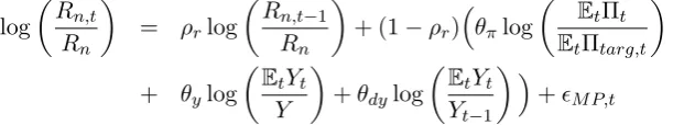
rate given by the following implementable Taylor-type rule:

log

Rn,t

Rn

= ρrlog

Rn,t−1

Rn

+ (1−ρr)

θπlog

Πt

Πtarg,t

+ θylog

Yt

Y

+θdylog

Yt

Yt−1

+M P,t (30)

logAt−logA = ρA(logAt−1−logA) +A,t

logGt−logG = ρG(logGt−1−logG) +G,t

logM St−logM S = ρM S(logM St−1−logM S) +M S,t

log Πtarg,t−log Π = ρπ(log Πtarg,t−1−log Π) +πtarg,t

andM P,tis an i.i.d. shock to monetary policy. Πtarg,tis a time-varying inflation target following

an AR(1) process. This completes the model.

3.4 Recovering the NK Workhorse Model

We now pose the question: can the linearized form of the non-linear model about the steady state reduce to the standard workhorse model in Section 2.1 where rational expectationsEtyt+1 and Etπt+1 or non-RE E∗tyt+1 and E∗tπt+1 can be treated as expectations by individual households

consider the linearized form of the above set-up about a zero inflation and growth deterministic steady state. With RE the householdj’s first order conditions take one of two forms. Either:

α1ct(j) = α2wt+α3(ω2,t+rt) +α4ω1,t (31)

ω1,t = α5Etwt+1−α6Etrt+1+βEtω1,t+1

ω2,t = (1−β)(γt−gt)−rt+βEtω2,t+1

γt =

1

γy

yt−

α

γy

(wt+ht)

from (20) where lower case variablesxt≡log(Xt/X) whereXis the steady state ofXt;cy ≡ _YC,

γy ≡ _YΓ,gy ≡ G_Y and γt isexogenous profit per household (a function of aggregate consumption

and hours). Positive coefficients are given by α1 ≡ 1 + _φcα_y, α2 ≡(1−β)(1 + _φ1)_cα_y, α3 ≡ γ_cyy,

α4 ≡ βα_cy,α5 ≡(1−β)(1 + 1_φ) and α6 ≡(1 +_φ1).

Alternatively from the Euler equation (13):

ct(j) =Etct+1(j)−Etrt+1 (32)

If now we make the assumption that households are identical and know this symmetric nature of the equilibrium then we have thatEtct+1(j) =Etct+1 which is now an expectation of a variable

exogenous to householdj. Then in a symmetric equilibrium.

ct=Etct+1−Etrt+1 (33)

Linearizing the household supply of hours decision, the resource constraint and the Fisher equation we have,

yt = (1−gy)ct+gygt (34)

rt = rn,t−1−πt+rst−1 (35)

ht =

1

φ(wt−ct)

Then in a special case where Gt = 0 and there is no distinction between public and private

consumption, gy = 0 and yt = ct. Equations (33)–(35) with rst = u1,t reduces to (1) where Etyt+1 is the forecast of aggregate output. With RE using (31) or (32) results in the same

equilibrium, but under bounded rationality with the same beliefs considered below this is no longer the case.

Turning to the supply side, for the wholesale sector:

yt = at+αht

mct = wt−yt+ht

For retail firmm, linearizing (24)–(26) and (27) about a zero net equation steady state we have:

po_t(m)−pt = βξEt[πt+1+pto+1(m)−pt+1] + (1−βξ)(mct+mst) (36)

Solving forward

po_t(m)−pt=Et

∞

X

i=0

(βξ)i[βξπt+i+1+ (1−βξ)(mct+i+mst+i)]

Then in a symmetric equilibrium we have

πt=

(1−ξ)

ξ Et

∞

X

i=0

(βξ)i[βξπt+i+1+ (1−βξ)(mct+i+mst+i)]

!

(38)

whereEt[πt+i+1] andEt[mct+i+mst+i] are expectations of aggregate inflation and real marginal

costs, both variables exogenous to individual price-setters. However, if we assume price-setters

know they are identical then we can use (37) to obtain

po_t(m)−pt=pot−pt=

ξ

(1−ξ)πt

Then substituting back into (36) we arrive at

πt=

(1−ξ)(1−βξ)

ξ E

∗

t

∞

X

i=0

βi(mct+i+mst+i) (39)

which omits learning about aggregate inflation. (39) is the familiar linearized Phillips curve. Under RE, (38) and (39) are equivalent. Puttingmct=wt−at+ht= (1 +φ)ht= (1 +φ)(yt−

at)/α, (39) in recursive form gives (2) withλ= (1−ξ)(1−_αξβξ)(1+φ) andu2,t =λmst.

To summarize, the ‘Euler Learning’ form of the workhorse linearized model expressed in terms of expectations of aggregate output (or the output gap) and inflation is valid under

bounded rationality provided that individual households and price-setting firmsknow the

sym-metric nature of the equilibrium. Then Euler learning is equivalent to internal rationality. If

we drop this assumption, then (31) and (38) must be used given non-RE beliefs of these same

aggregates and in addition expectations of the wage rate, interest rate, profits and government spending. This will be the form of the model we use under internal rationality.

4

Perfect versus Imperfect Information

We now examine the information assumptions that are made explicitly or implicitly in the RE and boundedly rational forms of the NK model. In linearized form of the NK model this can

has a state-space form:

"

zt+1 Etxt+1

#

= E

"

zt

xt

#

+

"

F

0

#

t+1; wt=G

"

zt

xt

#

(40)

whereztis a (n−m)×1 vector of predetermined variables at timetwithz0 given,xt, is am×1

vector of non-predetermined variables and wt is a vector observable macro-economic variables

which when we come to estimation will be the data used by the econometrician. All variables

tas a vector of random zero-mean shocks. RE under perfect information are formed assuming

a full information set{zs, xs, s},s≤t, E, F, G.

We now proceed to the assumption that there are non-rational agents who are unable to form model-consistent expectations. For such agents, in the learning literature pioneered by Evans and Honkapohja (2001) learning rules are specified in terms of the minimum state variable

representation of the perfect information model-consistent solution to (40). If the number of eigenvalues outside the unit circle is equal to the number of non-predetermined variables, the system has a unique equilibrium which is also stable with saddle-path xt = −N zt where

N =N(D) and depends on the rule (see Blanchard and Kahn (1980); Currie and Levine (1993)). Instability (indeterminacy) occurs when the number of eigenvalues of E outside the unit circle

is larger (smaller) than the number of non-predetermined variables.

Partitioning E conformably with zt and xt, the RE perfect information solution takes the

form of a first-order VAR

zt = [E11−E12N]zt−1+F t (41)

xt = −Nzt (42)

Etxt+1 = −NEtzt+1 =−N[E11−E12N]zt (43)

In the learning literature with ‘Euler-learning’ (also termed by Ellison and Pearlman (2011)

as ‘saddle-path learning’) agents are the assumed to make their forecast (43) by using (41) to estimate a first order VAR in zt. As we have seen this implies that agents know they are all

identical. But perfect information makes a further assumption that agents observe the state

vector including the shock processes.

We now express learning rules in terms of a subset of wt = [yt, πt, rn,t]0. Observing these

three time-series under RE enables agents (and the econometrician) to back out the shocks and to expresswt as an infinite VAR (Fernandez-Villaverde et al.(2007) and Levineet al. (2012)).

To show this write the RE solution as the following ARMA process

zt = Azt−1+Bt (44)

wt = Czt−1+Dt (45)

Because we have three shocks and three observables, the matrix D is square. Assume now it is also non-singular which is only possible if wt are observations without lags. Then t =

D−1_(w

t−Czt−1) and substituting into (44) and denoting the lag operator by L, we have

[(I−(A−BD−1C)L]zt=BD−1wt (46)

Hence combining (41) – (46) we have

zt =

∞

X

i=0

(A−BD−1C)iBD−1wt−i (47)

wt = C

∞

X

i=1

Convergence of the summations in (47) and (48) requires that the matrix (A−BD−1C) has all eigenvalues within the unit circle. Then equation (48) is an infinite VAR for the three observables

wt= [yt, πt, rn,t]0 which is estimatable from output, inflation and interest rate data.9 It follows

that the RE forecast is:

Etwt+1 = C

∞

X

i=0

(A−BD−1C)iBD−1wt−i (49)

whereas the adaptive heuristic rules (4) and (5) are parsimonious representations of (49):

E∗tyt+1 =

∞

X

i=0

λi_yyt−i; or E∗tyt+1=

∞

X

i=1

λi_yyt−i

E∗tπt+1 =

∞

X

i=0

λi_ππt−i; or E∗tπt+1 =

∞

X

i=1

λi_ππt−i

Thus we can interpret the heuristic rules as parsimonious forecasting models in which non-rational agents choose under-parameterized predictors (see Branch and Evans (2011)).

We conclude that unless shock processes are either known or observed then at best with the number of shocks equal to the number of observables and no lags in the latter, a well-specified

forecasting rule in the form of an infinite VAR is available and may be e-stable converging to the RE equilibrium.10 Otherwise the ARMA solution (44)–(45) is not invertible. In fact none of these conditions are satisfied in the set-up we consider when we come to estimation: we have

more shocks than observables and our heuristic rules assume aggregate variables are observed with a lag. Thus if we are to compare like with like, rational agents also observe with a lag and

we must therefore solve under imperfect information. We return to this issue in Section 8.

5

Internal Rationality

With internal rationality and anticipated utility (also known as the ‘infinite horizon approach’), our model of learning is one in which agents are rational regarding their internal decisions, but

have no macroeconomic model to form expectations of aggregate variables. We draw a clear distinction between aggregate and internal quantities so that identical agents in our model are

not aware of this equilibrium property (nor any others). We now drop the key assumption for Euler learning that agents know they are all identical.

We utilize the internal household and retail firm decision rules set out in Section 3.4. To

close the model, we need to specify the manner in which internally rational households and firms form their expectations. To do so, we assume that variables which are local to the agents,

in a geographical sense, are observable within the period, whereas variables that are strictly macroeconomic are only observable with a lag. This categorization regarding information about the current state of the economy follows Nimark (2014). He distinguishes between the local

information that agents acquire directly through their interactions in markets and statistics

9_{If this matrix is not stable, then the Spectral Factorization Theorem states that providedAis a stable matrix,} then there exists an infinite VAR representation; but in this case the estimated shocks are not the fundamental onest. See Fernandez-Villaverdeet al.(2007) for an example.

10

that are collected and summarised, usually by governments, and made available to the wider public.11 The only exception to this is the nominal interest rate, which we assume is observable within the period given the timing structure of NK models. Given this, we assume a strict form of naive expectations. Thus internally rational household expectations are given by

E∗trt+1 = rn,t−E∗tπt+1 (50)

E∗trt+i = rn,t+i−1−E∗tπt+i; i≥2 (51)

E∗trn,t+i = E∗trn,t+1; i≥1 (52) E∗h,tπt+i = E∗h,tπt+1; i≥1 (53)

E∗twt+i = E∗twt+1; i≥1 (54)

E∗tγt+i = E∗tγt+1; i≥1 (55)

Then expressing Etω1,t+1 and Etω2,t+1 in (31) as forward-looking summations and using (50)–

(55), we arrive at the IR consumption equation

α1ct = α2wt+α3(ω2,t+rt) +α4ω1,t

ω1,t =

1

1−β[α5E ∗

twt+1−α6(βE∗trn,t+1−E∗tπt+1)]−α6rn,t

ω2,t = (1−β)(γt−gt)−rt+

β

1−β((1−β)(E ∗

tγt+1−E∗tgt+1)−E∗trt+1)

which is now expressed in terms of one-step ahead forecasts by

E∗txt+1=Et∗xt+λx(xt−j−E∗txt) ; x=w, rn, π, γ; j= 0,1

Internally rational households make rational inter-temporal decisions for their consumption and

hours supplied given adaptive expectations of the wage rate, the nominal interest rate, inflation and profits. These macro-variables may in principle be observed with or without a one-period

lag (j = 1,0), but as stated earlier we assume j = 0 for market-specific variables wt, γt, and

j = 1 for aggregate inflation πt. However we assume the current nominal interest rate, rn,t is

announced and therefore also observed without a lag.

For retail firm m with adaptive expectations

E∗tπt+i+1 = E∗tπt+1; i≥0

E∗t(mct+i+mst+i) = E∗t(mct+1+mst+1) ; i≥1

so that

po_t(m)−pt=

βξ

1−βE ∗

f,tπt+1+ (1−βξ)(mct+mst) +

β

1−βE ∗

t(mct+1+mst+1)

One-step ahead forecasts are given by

E∗txt+1 =E∗txt+λx(xt−j−E∗txt) ; x=πf,(mc+ms); j= 0,1

11

Internally rational retail firms make rational inter-temporal decisions for their price and output given adaptive expectations of the aggregate inflation rate and their post-shock real marginal

shock wage rate. As before these variables may be observed with or without a one-period lag (j = 1,0), but for aggregate inflation we assume j = 1 as for households, but j = 0 for the market-specific variablemct. Note that we can in principle distinguish between households’ and

firms’ expectations of inflation.

6

Stability Analysis

We now have three possible models of expectations, rational (i.e. model consistent), boundedly

rational with Euler learning and boundedly but internally rational. We denote these three cases by RE, EL and IR respectively. In this section we consider homogeneous expectations for which all agents (households and firms) form either RE or IR or EL expectations. In the next section

we then allow for the possibility that households and firms are heterogenous across these groups (but retain intra-group homogeneity).

In the numerical results below we fix parameters at their priors used later in the Bayesian estimation apart from the adaptive learning parameter λx which we set at unity. As stated

above we make the following information assumptions: for observations of aggregate output

and inflationj= 1 which is assumed in the EL approach. Later in the IR approach we need to model observations ofmarket-specific variables consisting of factor prices, profits and marginal

costs. These we assume can be observed without a lag and therefore j = 0. Note this only applies to the EL and IR agents but the RE equilibrium for now assumes perfect information where agents observe all current values of state variables. Later in Section 8 we address this

inconsistency and assume all agents have the same imperfect information (II) set as for IR agents. However for rational agents the stability conditions considered now can be derived from a perfect foresight equilibrium and are independent of the information assumption.

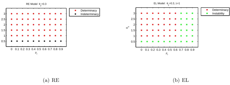
Figures 1 and 2 compare the models in (ρr, θπ) space with θy = 0.3 and θdy = 0. Finally

Figure 3 setsρr= 1 and compares EL and IR models in (αy, απ) space having re-parameterized

the rule as rn,t=ρrrn,t−1+αππt+αyyt. Note that this rule reduces to a price-level rule when

αy = 0. The differences in the sizes of the policy spaces that result in a saddle-path stable

equilibrium are significant. Furthermore a clear ranking of the sizes of these spaces emerges

with RE ⊃ EL ⊃ IR. This means that unless the policy rule is designed for the IR model, uncertainty as to which model of expectations is correct can lead to a rule that is unstable or

has infinite multiple equilibria (i.e., is indeterminate).

7

Heterogeneous Expectations across Households and Firms

Now we come to the full Brock-Hommes NK model but with IR rather than EL boundedly rational agents. The composite RE-IR model then has an equilibrium (in the original

non-linear form)

H_td = nh,t(Hts)RE+ (1−nh,t) (Hts)IR

0 0.1 0.2 0.3 0.4 0.5 0.6 0.7 0.8 0.9 0.5 1 1.5 2 2.5 3 ρr

RE Model θ_y=0.3

θπ

Determinacy Indeterminacy

(a) RE

0 0.1 0.2 0.3 0.4 0.5 0.6 0.7 0.8 0.9 0.5 1 1.5 2 2.5 3 ρ_r

EL Model: θy=0.3, λ=1

θπ

Determinacy Instability

(b) EL

Figure 1: Comparison of Stability Properties of RE and EL Models. ρr >0, λx = 1.

0 0.1 0.2 0.3 0.4 0.5 0.6 0.7 0.8 0.9 0.5 1 1.5 2 2.5 3 ρ_r

EL Model: θy=0.3, λ=1

θπ

Determinacy Instability

(a) EL

0 0.1 0.2 0.3 0.4 0.5 0.6 0.7 0.8 0.9 0.5 1 1.5 2 2.5 3 ρ_r

IR Model: θy=0.3, λ=1

θπ

Determinacy Instability

(b) IR

Figure 2: Comparison of Stability Properties of EL and IR Models. ρr >0, λx = 1.

0 0.25 0.5 0.75 1 1.25 1.5 1.75 2 0 0.1 0.2 0.3 0.4 0.5 0.6 0.7 0.8 0.9 1 1.1 1.2 αy

EL Model : Integral Interest Rate Rule

θπ

Determinacy Instability

(a) EL

0 0.25 0.5 0.75 1 1.25 1.5 1.75 2 0 0.1 0.2 0.3 0.4 0.5 0.6 0.7 0.8 0.9 1 1.1 1.2 αy

IR Model: Integral Interest Rate Rule

θπ

Determinacy Instability

(b) IR

Po t

Pt

= nf,t

Po

t

Pt

RE

+ (1−nf,t)

Po

t

Pt

IR

Note that rational agents in this model form model-consistent expectations taking into account the presence of internally rational agents.

We first consider the properties of the model with fixed exogenous proportions of RE and

IR agents. Then we allow these proportions to be determined endogenously. Finally we model the wealth distribution between RE and IR agents.

7.1 Exogenous Proportions of RE and IR Agents

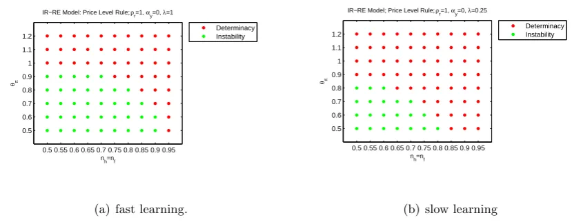
Figure 4 provides a stability analysis with a price level rule (ρr = 1, αy = 0 in the

re-parameterized rule rn,t = ρrrn,t−1 +αππt+αyyt), and nh = nf = n in the steady state.

We can see that fast learning (λx = 1) results in a larger regions of instability (a smaller policy

space) than the case of slower learning (λx= 0.25).

So far we have confined the simulations to parameter regions of the model and policy rule that result in saddle-path stability. If we enter a region of local instability, but global boundedness,

we see chaotic dynamics as highlighted generally in Hommes (2013) and for an NK model with Euler learning in Branch and McGough (2010). Two points should be made concerning this possible outcome. First, there is then enormous inflation volatility under chaos so the model

is one of hyper-inflation. Second, we have seen that this clearly undesirable outcome can be avoided by an appropriate choice of monetary policy rule.

0.5 0.55 0.6 0.65 0.7 0.75 0.8 0.85 0.9 0.95 0.5

0.6 0.7 0.8 0.9 1 1.1 1.2

n

h=nf

IR−RE Model: Price Level Rule; ρr=1, αy=0, λ=1

θπ

Determinacy Instability

(a) fast learning.

0.5 0.55 0.6 0.65 0.7 0.75 0.8 0.85 0.9 0.95 0.5

0.6 0.7 0.8 0.9 1 1.1 1.2

n

h=nf

IR−RE Model; Price Level Rule; ρr=1, αy=0, λ=0.25

θπ

Determinacy Instability

(b) slow learning

Figure 4: Stability of RE-IR heterogeneous-agent model with price-level rule under fast and slow learning.

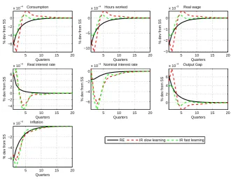
Figure 5 plots the impulse response functions (IRFs) with standard parameters for the rule for a shock to monetary policy under fast and slow learning. Figures 10 to 11 in the Online

Appendix show IRFs for shocks to technology and the mark-up shock. Not surprisingly fast learning sees an IRF converge faster to the RE case, but in either case IR introduces more

persistence compared with RE. This suggests this feature should lead to a better fit of the data

5 10 15 20 −6

−4 −2 0

x 10−4

Quarters

% dev from SS

Consumption

5 10 15 20 −10

−5 0

x 10−4

Quarters

% dev from SS

Hours worked

5 10 15 20 −3

−2 −1 0

x 10−3

Quarters

% dev from SS

Real wage

5 10 15 20 −4

−2 0 2 4 6

x 10−4

Quarters

% dev from SS

Real interest rate

5 10 15 20 −6

−4 −2 0

x 10−4

Quarters

% dev from SS

Nominal interest rate

5 10 15 20 0

2 4 6

x 10−4

Quarters

% dev from SS

Output Gap

5 10 15 20 −6

−4 −2

x 10−4

Quarters

% dev from SS

Inflation

RE IR slow learning IR fast learning

Figure 5: RE versus RE-IR Composite Expectations withnh=nf = 0.5, λx= 0.25,1.0;

Taylor rule with ρr = 0.7, θπ = 1.5 and θy = 0.3, θdy = 0, Monetary Policy Shock

7.2 Endogenous Proportions of RE and IR Agents

Proportions of rational households and firms are given by

nh,t =

exp(−γΦRE_h,t)

exp(−γΦh,t)RE+ exp(γΦIRh,t)

nf,t =

exp(−γΦRE_f,t) exp(−γΦRE

f,t) + exp(γΦIRf,t)

where fitness for households given by

ΦRE_h,t = µRE_h ΦRE_h,t−1+

weighted sum of forecast errors +Ch

ΦIR_h,t = µIR_h ΦIR_h,t−1+weighted sum of forecast errors

with similar expressions for firms with a subscriptf replacingh. Using the estimated model of

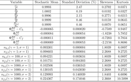
the next section, Table 1 provides a third order perturbation solution of non-linear NK RE-IR Model. In the estimation the model is linearized and the proportions nh,t and nf,t are fixed.

Non-linear estimation is required to pin down the parameters nh, nf in the steady state, and

µRE,IR_h ,µRE,IR_f andγin the reinforcement learning process. So here we impose them as reported in the table. We also scale the estimated standard deviations of the shocks using a parameter

Variable Stochastic Mean Standard Deviation (%) Skewness Kurtosis

Ct

C 0.9993 2.47 0.2792 0.0371

Ht

H 1.0002 0.19 0.0192 0.0327

Wt

W 0.9996 2.15 0.2771 0.0215

Πt

Π 0.9999 0.46 0.0159 0.0645

Rn,t

Rn 0.9999 0.46 0.0070 0.0651

ΦRE_h,t −Ch -0.000065 0.000020 -0.7589 0.9487

ΦAE_h,t -0.000084 0.000054 -1.8238 5.7852

ΦRE_f,t −Cf -0.000011 0.000009 -0.7203 0.7834

ΦAE

f,t -0.000069 0.000053 -2.2156 8.8686

nh,t(γ = 1;σ = 1) 0.093301 0.000004 1.8039 6.0897

nf,t(γ = 1;σ= 1) 0.098603 0.000004 2.2688 9.2725

nh,t(γ = 100;σ = 1) 0.094221 0.003634 1.8039 6.0897

nf,t(γ = 100;σ= 1) 0.101751 0.004303 2.2688 9.2725

nh,t(γ = 1000;σ = 1) 0.102506 0.036343 1.8039 6.0897

nf,t(γ = 1000;σ = 1) 0.130105 0.043030 2.2688 9.2725

nh,t(γ = 1000;σ = 2) 0.129993 0.146939 1.8403 6.6096

nf,t(γ = 1000;σ = 2) 0.224367 0.174046 2.3668 10.5098

Table 1: Third Order Solution of the Estimated NK RE-IR Model; µRE_h = µIR_h =

µRE

f =µIRf = 0.0;γ = 1,100,1000

introduceshigh kurtosis and skewness12 in macro variables and learning results in the numbers of rational agents increasing from the estimated deterministic steady state value of 0.093 and

0.099 to 0.13 and 0.22 for households and firms respectively in the stochastic steady state.

7.3 Wealth Distribution

Up to now we have assumed that there is no net lending of borrowing between each of the RE and IR households. We now relax this assumption and allow for a wealth distribution between

these groups. To achieve a stationary path for bond holdings we need to introduce a portfolio adjustment cost. Consider thejth RE household with a budget constraint:

B_tRE(j) =RtBREt−1(j) +WtHt(j)RE+ Γt−Ct(j)RE−Tt−

$

2(B

RE

t−1(j)−B)2

Then zero net wealth in aggregate implies thatnh,tBtRE =−(1−nh,t)BtIR.

Define the Lagrangian at time t= 0 as

Et

h_X∞

t=0

βt[U(C_tRE(j), H_tRE(j))

+ λt(RtBtRE−1(j) +WtHtRE(j)−Γt−CtRE(j)−Tt−

$

2(B

RE

t−1(j)−B)2)−BtRE(j)]

i

Then givenB₀RE(j) the first order conditions are

C_tRE : U_CRE(j)−λt= 0

B_tRE : Et

βλt+1(Rt+1−$(BtRE(j)−B))−λt

= 0

Hence the consumption Euler equation becomes

Et

"

βU

RE

C,t+1(j)(Rt+1−$(Bt(j)−B))

UC,t(j)

#

=Et

ΛRE_t,t+1(j)(Rt+1−$(BREt (j)−B))

= 1

The remaining change to the model is to replace C_tIR withC_tIR−B_tIR.

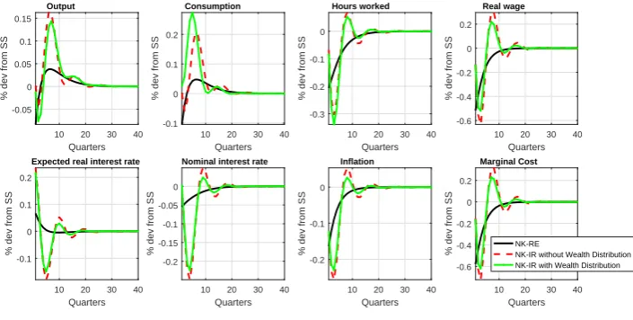
With the same choice of parameter values as before and $chosen to be very small, Figure 6 compares the impulse responses of the RE model with the heterogeneous agent RE-IR model

with exogenous and equal proportions of RE and IR households and firms. Figures 12–13 in the Online Appendix provide impulse response functions for technology and government spending

shocks. The case where the wealth distribution between RE and IR households is included is compared with that where (as in all the heterogeneous NK model literature) it is suppressed. The figures suggest that with our calibration the wealth distribution effect does not significantly

change the equilibrium, at least up to first order for which the impulse responses are computed.

10 20 30 40 Quarters -0.05 0 0.05 0.1 0.15

% dev from SS

Output

10 20 30 40 Quarters -0.1

0 0.1 0.2

% dev from SS

Consumption

10 20 30 40 Quarters -0.3

-0.2 -0.1 0

% dev from SS

Hours worked

10 20 30 40 Quarters -0.6 -0.4 -0.2 0 0.2

% dev from SS

Real wage

10 20 30 40 Quarters -0.1

0 0.1 0.2

% dev from SS

Expected real interest rate

10 20 30 40 Quarters -0.2 -0.15 -0.1 -0.05 0

% dev from SS

Nominal interest rate

10 20 30 40 Quarters -0.2

-0.1 0

% dev from SS

Inflation

10 20 30 40 Quarters -0.6 -0.4 -0.2 0 0.2

% dev from SS

Marginal Cost

NK-RE

NK-IR without Wealth Distribution NK-IR with Wealth Distribution

Figure 6: Wealth Distribution and Impulse Responses – Monetary Policy Shock

8

Bayesian Estimation

We now turn to the estimation of an empirical NK behavioural model which differs from the

linearized form used up to now in two respects: first, we assume that the a steady state about which the perturbation solution is computed has a non-zero net growth and inflation. The former is stochastic and given by gt = (1 +g) exp(Atrend)−1 where Atrend is a shock to

expectations assumption used by IR agents in the previous section drawing upon Hommeset al. (2015), Anufrievet al.(2015) and Hommes (2011). For any variable with outcomeXt we study

heuristic forecasting rules of the form:

X_te=Xλ1

t−1(Xte−1)1−λ1

Xt−1

Xt−2

λ2

; λ1 ∈[0,1], λ2∈[−1,1]

where X_te ≡ E∗t−1Xt. If we put λ2 = 0, this reduces to the adaptive expectations case of the

previous sections.

We estimate three models with wealth distribution: the NK RE model, the NK model with

individual rationality (IR Model) and the behavioural composite model with heterogeneous expectations (RE-IR Model). For the RE agents in either the ‘pure’ or composite RE model we assume and compare perfect or imperfect information sets as discussed in Section 4. Bayesian

methods are employed using Dynare adapted to handle imperfect information.13 We use a subset of the observable set used in Smets and Wouters (2007) in first difference at quarterly

frequency but extend the sample length to the second quarter of 2008, before the outbreak of the 2008-09 crisis. Thus the sample period is 1984:1-2008:2. These observable variables are the log differences of real GDP and the GDP deflator, and the federal funds rate. All series are

seasonally adjusted and taken from the FRED Database available through the Federal Reserve Bank of St.Louis and the US Bureau of Labour Statistics.

8.1 The Measurement Equations and Priors

The corresponding measurement equations for the 3 observables are:14



 

D(logGDPt)∗100

log(GDP DEFt/GDP DEFt−1)∗100

F EDF U N DSt/4∗100



 =



  

logYt Yt

−logYt−1

Yt−1

+ trend +y,t−y,t−1+A,t

log Πt

Π

+ consπ+π,t

logRn,t Rn

+ consr



  

where constants trend,consπ and consr are related to the steady state of our model by

Π = consπ/100 + 1

log(1 +g) = trend/100

Rn =

Π

βg

= Π(1 +g)

β = consr/100 + 1

This implies thatβ is determined empirically as

β=

consπ + 100

consr+ 100

(1 +g)

We introduce measurement errors on two observables, output and inflation (y,tand π,t) so

in total there are 3 variables in the observations, 4 exogenous AR(1) processes (At,Gt,M St,

Πtarg,t) and 4 further i.i.d shocks including measurement errors, (M P,t,Atrend,t and y,t,π,t).

13

Levineet al.(2017a) provides full details of this addition to Dynare. 14

Yt=GDPt,Yt=trend and trend growth =logYt−logYt−1= log(1+g)+A,t. y,tandπ,tare measurement

Thus there are 8 shocks and 3 observables meaning that the invertibilty condition discussed in Section 4 is not satisfied. A number of the structural parameters are fixed, so as to match their

sample means or in accordance with previous studies and are collected into Θf:

Θf ≡[ζ, α, µREh , µIRh , µREf , µIRf , γ] = [7.0,0.7,0.5,0.5,0.5,0.5,1.0]

These parameters are necessary to solve and linearize the models but are problematic for estima-tion (e.g. identificaestima-tion). From Secestima-tion 7 the parameters in the RE-IR model, [µRE_h µIR_h µRE_f µIR_f γ], do not enter into the first-order solution for the linearized model but only affect the second-order or higher solutions. They cannot be identified in the first-second-order solution that is used for estimation so are imposed at their mid-point values as above. As in De Grauwe (2011) we fixγ

to unity so that allow for a moderate degree in the intensity of individual choice. The remaining calibration values for [ζ, α] are standard choices in the DSGE literature.

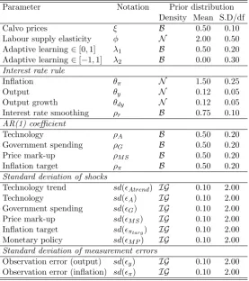
For the remainder of parameters gamma and inverse gamma distributions are used as priors when non-negativity constraints are necessary, and beta distributions for fractions or probabil-ities. Normal distributions are used when more informative priors seem to be necessary. The

prior means and distributions of these parameters can be found in Table 2. The values of priors are in line with those in Smets and Wouters (2007). The Calvo coefficient ξ is assumed to be beta distributed with prior mean of 0.5 and prior standard deviation of 0.2, implying that

prices are sticky for two quarters. We draw all the AR(1) parameters ρA, ρM S, ρπ and ρG,

and the lagged interest rate ρr from the beta distribution in order to restrict them to the open

unit interval. Similarly, the beta distribution we use on the adaptive expectations learning parameter λ1 also restricts it to the open unit interval, but we set a generalized beta prior for

λ2 with support [−1,1] and 0 mean. For all these beta distribution parameters we centre the

prior density in the middle of the unit interval.

A common theme in papers that study empirical RBC/DSGE models is the difficulty in

pinning down the parameter of labour supply elasticity φ. Inference on the inverse Frisch elasticity of labour supply has been found susceptible to model specifications, and exhibiting wide posterior probability intervals. So we assume a normal distribution with mean 2.0 and

standard deviation of 0.5 for the parameter which is well within the range of point estimates reported in the RBC and labour literature. For the Taylor rule parameter on inflation the prior is set to obey the Taylor principle is centred at the value suggested by Taylor. With

regard to output level and growth the response of interest rate is smaller but we do not rule out negative responses for both parameters. Finally the priors on the standard deviations of the

exogenous shocks and measurement errors are assumed to have inverse gamma distributions. The uncertainty held about these elements motivates an open interval for their priors that excludes zero and is unbounded.

8.2 Identification Checks and Estimation of the Posterior Distribution

Based on the prior information, we first conduct some pre-estimation identification diagnostics

and report them in detail in Appendix D. We find that the sensitivity effect ofnf at its posterior

mean point is relatively weak and also at their estimated values, the pair-wise collinearity

Parameter Notation Prior distribution Density Mean S.D/df

Calvo prices ξ B 0.50 0.10

Labour supply elasticity φ N 2.00 0.50 Adaptive learning∈[0,1] λ1 B 0.50 0.20

Adaptive learning∈[−1,1] λ2 B 0.00 0.30

Interest rate rule

Inflation θπ N 1.50 0.25

Output θy N 0.12 0.05

Output growth θdy N 0.12 0.05

Interest rate smoothing ρr B 0.75 0.10

AR(1) coefficient

Technology ρA B 0.50 0.20

Government spending ρG B 0.50 0.20

Price mark-up ρM S B 0.50 0.20

Inflation target ρπ B 0.50 0.20

Standard deviation of shocks

Technology trend sd(Atrend) IG 0.10 2.00

Technology sd(A) IG 0.10 2.00

Government spending sd(G) IG 0.10 2.00

Price mark-up sd(M S) IG 0.10 2.00

Inflation target sd(πtarg) IG 0.10 2.00

Monetary policy sd(M P) IG 0.10 2.00

Standard deviation of measurement errors

Observation error (output) sd(y) IG 0.10 2.00

Observation error (inflation) sd(π) IG 0.10 2.00 Table 2: Prior Distributions

high correlations to near-exact collinearity one may suspect some weak identification. Figure 15 in the Online Appendix shows the identification strength and sensitivity component in the

moments using the composite RE-IR estimation results and shows again the sensitive strength in the moments of nh is very weak. Therefore in this section we compare the cases without

estimatingnf and nh so the proportionsnh =nf =n= 0.5,0.1 are fixed to the values we used

in the stability section earlier in the paper.

Turning to the estimation, the joint posterior distribution of the estimated parameters is

obtained in two steps. First, the posterior mode and the Hessian matrix are obtained via standard numerical optimization routines. The Hessian matrix is then used in the Metropolis-Hastings (MH) algorithm to generate a sample from the posterior distribution. Two parallel

chains are used in the Monte-Carlo Markov Chain Metropolis-Hastings (MCMC-MH) algorithm. Thus, 100,000 random draws (though the first 25% ‘burn-in’ observations are discarded to

remove any dependance from the initial conditions) from the posterior density are obtained via the MCMC-MH algorithm, with the variance-covariance matrix of the perturbation term in the algorithm being adjusted in order to obtain reasonable acceptance rates (between

20%-40%). We run an iterative process of MCMC simulations in order to calibrate the scaling factor to achieve the desired rate of acceptance which is key for the speed of convergence of the MCMC-MH chains, which are also sensitive to the number of MCMC iterations. The former

ensures that more of the parameter region is searched more regularly, but at the expense of reducing the acceptance ratio. In this estimation the number of draws we choose is sufficient to

acceptance rate, we use the convergence indicators recommended by Brooks and Gelman (1998) and Gelman et al. (2003).

8.3 Bayes Factor Comparison

We first focus on the pure RE, pure IR and the composite RE-IR models when RE agents have a

perfect information set. We employ the Bayes Factor (BF) from the model marginal likelihoods to gauge the relative merits across the four models in Table 3.

Model Pure RE (PI) Pure IR RE(PI)-IR (n=0.5) RE(PI)-IR (n=0.1)

LL -143.05 -138.90 -139.38 -138.15

Prob 0.0042 0.2666 0.1649 0.5643

Table 3: Marginal Log-likelihood Values and Posterior Model Odds: RE Agents

with Perfect Information (PI)

Models IR (Pure IR) and RE-IR (n= 0.1,0.5) all substantially outperform their RE coun-terpart which is firmly rejected by the data. Formally, using the Bayesian statistical language of Kass and Raftery (1995), a BF, the quotient of the probabilities reported, greater than 100

(marginal log-likelihood difference over 4.61) offers “decisive evidence”. Thus we have decisive support for the pure IR and some composite behaviour from the US data we observe. However

the BF differences between the non-RE models are not strong.

Next we assume an imperfect information set for the RE agents of the form:

It= [Ys−1,Πs−1, Rn,s;s≤t]

The policy maker is assumed observe current output, inflation and to know to know her own

current inflation target. The implemented rule therefore is still (30), but theperceived rule for RE agents with II, again imposing point expectations, is now given by the rule:

log

Rn,t

Rn

= ρrlog

Rn,t−1

Rn

+ (1−ρr)

θπlog

EtΠt EtΠtarg,t

+ θylog

EtYt

Y

+θdylog

EtYt

Yt−1

+M P,t (56)

where rational expectations under II of current inflation, output and the inflation target are now required to implement the rule. An important point to stress is that this is the same

information set we assume for IR agents when they come to update their heuristic rule. In

this sense we now have informational consistency across IR and RE agents, and also with the

econometrician estimating the model. This feature we believe is new for the heterogeneous behavioural NK model literature.15 The results for the likelihood race are reported in Table 4.

15

If we assume informational consistency for the policymaker as well then her information set would beIt=

[Ys−1,Πs−1, Rn,s,Πtarg,t]. Then the implemented rule becomes (56), rather than (30), but withEtΠtarg,treplaced

with Πtarg,t(since the policymaker knows her own target). But then the set-up involvestwoimperfect information

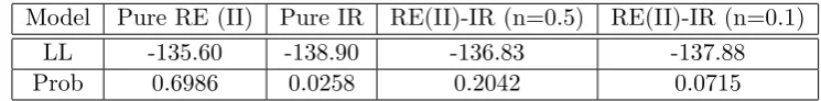
Model Pure RE (II) Pure IR RE(II)-IR (n=0.5) RE(II)-IR (n=0.1)

LL -135.60 -138.90 -136.83 -137.88

Prob 0.6986 0.0258 0.2042 0.0715

Table 4: Marginal Log-likelihood Values and Posterior Model Odds: RE Agents

with Imperfect Information (II)

Now a very different picture emerges when comparing the RE model with the behavioural

alternatives. RE with imperfect information (RE(II)) actually wins the likelihood race. In formal Bayesian language, a BF of 10-100 or a marginal likelihood range of [2.30, 4.61] is “strong to very strong evidence” so the RE(II) strongly dominates the pure II and RE(II)-IR

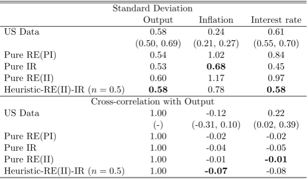
with n=0.1. But the likelihood race cannot separate the RE(II) and RE(II)-IR composite model with n=0.5. In Section 9 we examine whether the ability to match second moments of the data is able to separate these two models. But first we turn to the parameter estimation results.

8.4 Parameter Estimation Results

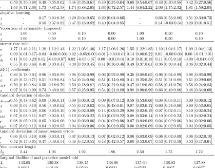
Table 5 contains summary statistics of the posterior distributions of the NK models. We

re-port posterior means of the parameters of interest and 95% probability intervals alongside the posterior model odds for all 7 models so far: RE(PI), RE(II), IR and RE(PI)-IR or RE(II)-IR

withn= 0.5,0.1.

The price stickiness parameter, ξ, is estimated to be larger than assumed in the prior distribution (0.59). This implies that there is some degree of price stickiness and the implied

average contract duration is about 2.44 quarters from this model. The posteriors of this model also indicate a Frisch labour supply elasticity, φ−1 = 0.61 and a strong response to inflation that satisfies the Taylor principle, θπ = 1.77. In terms of the persistence of the exogenous

shocks, the estimates of the AR(1) coefficients show that the technology and inflation shocks are inertial. According to the estimated standard deviation, the technology shock stands out as

being the most volatile structural shock in this economy. The interest rate policy shock is less volatile and is less important in driving inflation, consumption and output. The variations in

measurement error of output is relatively moderate in this model but there is a sizeable estimate of the inflation measurement error. Overall these estimates are in the range often found in the existing literature.

The IR solution equilibrium we propose departs from the standard RE solutions and allows a process of adaptive learning driven by the speed of learning parameterλ1 ∈[0,1] andλ2 ∈[−1,1]

for the household and firms respectively. The closer λ is to zero slower the learning process

is, which is the key mechanism of this setup because this introduces more dynamics into the model.

Focusing on the parameter characterising the degree of price stickiness, ξ, again, the mean estimates report an average price contract duration of around 1.96 and 1.92 quarters for IR and RE-IR. Their estimated 95% intervals imply that price contacts change in the ranges of

∈(1.54,2.50) suggesting that the firms of IR and RE-IR economies change prices as frequently

as once every 1.5 quarters. The estimated contract length is shorter in the non-pure-RE models.