On the use of positive polynomials for the estimation of upper and lower expectations in orbital dynamics

On the Use of Positive Polynomials for the

Estimation of Upper and Lower Expectations in

Orbital Dynamics

Massimiliano Vasile and Chiara Tardioli

AbstractThe paper presents the use of positive polynomials, in particular Bernstein polynomials, to represents families of probability distributions in orbital dynamics. The uncertainty in model parameters and initial conditions is modeled with p-boxes to account for imprecision and lack of knowledge. The resulting uncertainty in the quantity of interest is estimated by representing the upper and lower expectations with positive polynomials with interval coefficients. The impact probability of an asteroid subject to a partially known Yarkovsky effect is used as an illustrative ex-ample.

1 Introduction

The treatment of uncertainty in orbit propagation is of fundamental importance to predict the motion of natural and man-made objects. In the specific case of asteroids and space debris a key quantity of interest is the probability of an impact with the Earth or a collision with an operational satellite.

Several methods have been proposed to deal with uncertainty and provide a pre-diction of the future state of a space object. Most of them start from some assump-tions on the probability distribution associated to the uncertain quantities and then model, more or less accurately, the distribution of the quantity of interest. When the nature of uncertainty is epistemic (lack of knowledge), a single probability dis-tribution might not be available. More likely different sources of information may suggest that the probability associated to an uncertain quantity belongs to a finite set for which we can define upper and lower bounds.

However, the fast calculation of these bounds is not a trivial matter. In this pa-per an approach based on the use of positive polynomials is proposed to calculate

Massimiliano Vasile, Chiara Tardioli

Aerospace Centre of Excellence, University of Strathclyde, 75 Montrose Street, G11XJ, Glasgow, UK, e-mail: [massimiliano.vasile - chiara.tardioli]@strath.ac.uk

the upper and lower bounds via a simple linear optimisation programme. The un-certain quantities are modeled with p-boxes defined through parametric probability distributions or via positive polynomial expansions [4].

The calculation of the impact probability of an asteroid subject to a poorly known Yarkovsky effect is used as an illustrative example.

2 Worst Case Scenario

The problem under investigation is to evaluate the probability of the following set of events:

Aν={u∈U0 : f(u)≤ν} (1)

where f is the quantity of interest anduis a stochastic variable defined in an un-certainty spaceU0with dimensiond. We use the notation[u]∈Rdto indicate the convex set ofusuch thatu∈U₀⊆Rd. Ifd=1, the uncertainty is an interval and it is also indicated as[u,u], whereu,uare the lower and upper limit, respectively.

Regardless of the distribution ofuone can define the best and worst case scenar-ios as follows:

f =min

u∈U0

f(u), f =max

u∈U0

f(u). (2)

The solution to (20) gives the limit of variability of f and identifies also two rare events. For any value ofν∈[f,f]and a known probability distributionp, the prob-ability associated toAνis given by the formula

IP(Aν) = Z

Aν

p(u)du, (3)

In the following, the uncertain variables are assumed to be independent and un-correlated so that the initial uncertainty space is the hyper-rectangle, however, the solution of Eqs. (20) does not requireU0to be a box and holds true for any generic set. The same is true for Eq.(22).

3 Upper and Lower Expectations

3.1 Representation with Families of Parametric Distributions

Consider the case in which one can reasonably assume that the uncertainty can be quantified with a family of beta distributions with unknown parametersαandβ(any other parametric or non-parametric distribution would equally work). Eq. (22) then translates into two equations defining the upper and lower probability associated to Aν:

min α,β

Z

Aν

p(u)du, max α,β

Z

Aν

p(u)du, (4)

where p is the product of probability p=∏dj=1pj, where each marginal density

masspjis a beta distribution function with parametersαj,βj.

3.2 Representation with Positive Polynomials

In the general case the integrals in Eqs.(4) can calculated numerically via multidi-mensional quadrature formula. As an example we can replace the calculation of the exact integrals with an approximation using Halton low discrepancy sequence to generateMsample points (called quasi-Monte Carlo points) in the domainU0and then re-write the integrals in the form:

Z

Aν

p(u)du≈ 1

M

M

∑

k=1

IAν(uk)p(uk) (5)

where the samplesuk are taken from the low discrepancy sequence. Similarly, we

can approximate the integrals in Eq. (4):

min α,β

M

∑

k=1

IAν(uk)

∏

pj(uk), max

α,β

M

∑

k=1

IAν(uk)

∏

pj(uk). (6)

subject to the constraint:

1 M

M

∑

k=1

p(uk) =1. (7)

If the family of distributions is unknown or does not contain only one particular type, one can use an a representation with an expansion in positive polynomials to approximate the extrema of[p]and obtain the upper and lower expectation onAν as solutions of a linear problem. In this paper, in particular, we propose the use of Bernstein polynomials [4][7]. The family of probability distributions to which the uncertain variableujbelongs can be expressed as

[pcj] =

n n

∑

i=1

c(_ij)Bi(τj(uj)) o

whereBi:[0,1]7→[0,1]is theith-univariate Bernstein polynomials of dimensionn

andτjis the change of coordinate from the uncertain interval[uj]to[0,1].

Under the independence and non-correlation assumption among the variables, the joint probability distribution is the product of the marginal masses and it is con-tained in the p-box[pc˜] =∏dj=1[pcj]which can be re-written as

[pc] = n

∑

cκBκ(τ(u))

o

, (9)

withK ={κ= (k1, . . . ,kd)∈Nd: 0≤kj≤n,∀j},Bκ is a multivariate Bernstein polynomial,τ=∏dj=1τj, andcis the unknown coefficient vector. Then, the upper

and lower expectation are the solutions of the two linear optimization problems:

E_l(Aν) =min

c∈C Z

Aν

pc(u)du, Eu(Aν) =max

c∈C Z

Aν

pc(u)du, (10)

The setC ∈RMcan be assumed to be an hyper-cube, for example,C = [0,M]M. In discrete form programmes (10) translate into:

El(Aν) =min

c∈C

M

∑

s=1

IAν(us)

∑

κ∈K

cκBκ(τ(us)), (11)

and

Eu(Aν) =max

c∈C

M

∑

s=1

IAν(us)

∑

κ∈K

cκBκ(τ(us)). (12)

subject to the linear constraint:

1 M

M

∑

s=1κ

∑

cκBκ(τ(us)) =1. (13)

3.3 Impact probability

Positive polynomials are here applied to the estimation of upper and lower impact probabilities of an asteroid subject to the Yarkovsky effect.

We consider a simplified dynamical model of an asteroid under the gravitational force of the Sun and of the Yarkovsky effect. The latter is assumed to be a purely transverse accelerationA2/r2, whereris the heliocentric distance andA2is a func-tion of the asteroid physical quantities[3]. The dynamical equafunc-tions, expressed in Keplerian orbital elements, can be reduced to

da dt =

2A2(1−e2)

np2 ,

dM

whereeis the eccentricity,Mis the mean anomaly,n=pµ/a3_{is the mean motion} of the unperturbed orbit withµthe gravitational parameter, andp=a(1−e2)is the conic parameter. ForA2=0 the dynamics (14) reduces to a pure Keplerian motion, while the semi-major axis drifts outwards forA2>0, and inwards forA2<0.

AlthoughA2is unknown, it can be estimated using the available information on the physical model. Following Farnocchia et al.[3], the coefficientA2is expressed as

A2=

4(1−A)

9 Φ(1au)f(Θ)cosγ, f(Θ) =

0.5Θ

1+Θ+0.5Θ2, (15) whereΦ(1au)is the standard radiation force factor at 1 astronomical unit, A is the Bond albedo,Θis the thermal parameter, andγis the obliquity. The radiation force at 1 W/m2is computed as

Φ(r) = 3L0

2cρD, (16)

whereL0is the luminosity of the Sun, i.e., the total power output of the source,Ris the mean radius of the asteroid,mathe mass of the asteroid, andcis the velocity of

light.

Using Bowel et al.[1], the Bond albedo can be written asA= (0.29+0.684G)pv, withGthe slope parameter andpvthe geometric albedo. Farnocchia et al.[3] related the thermal parameterΘ to the thermal inertiaΓ:

Θ= Γ ε σT3

ss r

2π

Prot

, (17)

whereεis the emissivity coefficient,σis the Stefan-Boltzmann constant,Prot is the

rotation period, andTssis the subsolar temperature[2]

Tss=

_(1−A)L

0

η ε σr2

1/4

, (18)

wherer is the heliocentric distance of the body and η is the so-called beaming parameter, which is equal to one in the case that each point of the surface is in instantaneous thermal equilibrium with solar radiation.

Delb`o et al.[2] related the thermal inertia to the diameterD(in km) by the ex-pression

Γ =d0D−ψ,

withd0=300±45 Jm−2s−1/2K−1andψ=0.36±0.09.

Eventually, the diameter can be related to the absolute magnitude H and the geometric albedo by the formula[6]

D=132910 −H/5

√

pv

. (19)

Therefore, both the inward and the outward drift of the semi-major axis are pos-sible. In addition, other key physical parameters are known with uncertainty. Due to the lack of knowledge in their distributions, they need to be treated as epistemic uncertainty variables.

It is assumed that both the initial conditions and the model parameters are uncer-tain. The uncertainty space isU0= [x0]×[q]⊂R10, wherex0= (a0,e0,I0,Ω0,ω0, `0) is the initial Keplerian orbital element vector, andq= (D,G,pv,ρ,d0,ψ,Prot,γ)is the model parameter vector.

The impact risk is computed at the close approach epoch using the projection on the target plane and the impact parameterb. We say that a collision may occur if the b-parameter is less or equal a safety radius:b≤R∗; this threshold is fixed here at 1.5 Earth radii.

Due to the uncertainty in the initial conditions, the final states of the asteroid defined a connected region more or less elongated along its orbit. Therefore, we say that the significant uncertainty of the b-parameter is contained in the interval

[b,b]⊆Rgiven by

b=min

u∈U0

b(u), b=max

u∈U0

b(u). (20)

Assuming that the orbital elements are uncertain with known distributions (aleatory uncertainty), while the model parameters are uncertain with unknown distributions (epistemic uncertainty), the product of their probabilities is epistemic and it is indi-cated with the probability box (shortly, p-box)[p]. Then the upper and lower impact probabilities is given by the formula

Pu(AR∗) =max

p∈[p]

Z

AR∗

p(u)du, (21)

Pl(AR∗) =min p∈[p]

Z

A_R∗

p(u)du, (22)

whereAR∗ ={u∈U0: b(u)≤R∗}is the event of interest.

We can now assume that each uncertainty variables is contained in a probability box (p-box) delimited by two Beta distribution functions:

[pi] ={cdfBeta(α,β) : 1≤α,β≤3},

whereiis the variable index. This is the situation in which there are two experts with opposite opinions: one believes that the most probable value is the left extrema of the interval (Beta(1,3)) and the other that most probable value is the right extrema of the interval (Beta(3,1)); and in the uncertainty analysis we want to take into account both of them. Each p-box can be re-defined as in Eq. (9) with Bk,k=1, . . . ,M

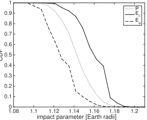
Figure 1 shows the cumulative distribution function of the b-parameter corre-sponding to an aleatory and epistemic case. CurvePrepresents the case when all variables are aleatory with known Beta distributions with parametersα=3,β =3 for the orbital elements and Beta functionsα=1,β=1 (uniform distribution) for the Yarkovsky parameters. On the contrary when uncertainty on the model parame-ters and initial conditions is epistemic one obtains the upper and lower expectations (curvesEuandEl, respectively). For all the possible values of the uncertain

param-eters the impact probability in Eq. (22) is 1 since b≤1.5R⊕, withR⊕ the Earth radius, for everyb.

impact parameter [Earth radii]

1.08 1.1 1.12 1.14 1.16 1.18 1.2

CDF

0 0.1 0.2 0.3 0.4 0.5 0.6 0.7 0.8 0.9 1

P E_l E_u

Fig. 1: Impact probability before deflection

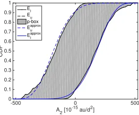
From the same analysis one can estimate an upper and lower expectation of the Yarkovsky parameterA2. Following Section 3.2, we can solve Eq. (10) with C =

[0,M]M,M=6,561, and the integral approximation given by Eq. (6) on 2·105 quasi-Monte Carlo samples. The upper and lower expectation delimiting the p-box are computed on 50 bins in the interval[−524,524]au/d2, using Bernstein polynomials as described in Section 3.2 on 104quansi-Monte Carlo points. The p-box ofA2is shown in Figure 2. The Yarkovsky parameter is computed at a fixed distance of a√1−e2_{. In the dynamical model we will sampleA}

2from distributionsPsuch that El ≤P≤Eu. To simplify the problem the upper and lower expectation have been

approximated by Beta functions (Figure 2):

Eu≈cdfBeta(5,10) El≈cdfBeta(10,5).

4 Conclusion

A

2 [10 -15 _au/d2_]

-500 0 500

CDF

0 0.1 0.2 0.3 0.4 0.5 0.6 0.7 0.8 0.9 1

E_l E_u p-box E_uapprox

E_lapprox

Fig. 2: Upper and lower expectation of the Yarkovsky parameter A2

single linear constraint. The use of Bernstein polynomials, as proposed in this paper, allows for the representation of any set of probability distributions with finite sup-port. The main limitation is the exponential growth of the number of polynomial co-efficients with the number of dimensions. However, this problem is equally present in Gaussian mixture models although in this case no parameters, appearing nonlin-ear in the mixture model, need to be defined. The number of terms in the expansion can be calibrated to achieve the desired representation. Furthermore, the approach in this paper can be applied in conjunction with an high-dimensional representation of the quantity of interest that would mitigate the curse of dimensionality.

Acknowledgment

The work in this paper was partially supported by the Marie Curie FP7-PEOPLE-2012-ITN Stardust, grant agreement 317185.

References

1. Bowell, E., Hapke, B., Domingue, D., Lumme, K., Peltoniemi, J., Harris, A.W.: Application of photometric models to asteroids. In: R.P. Binzel, T. Gehrels, M.S. Matthews (eds.) Asteroids II, pp. 524–556 (1989)

2. Delb`o, M., dell’Oro, A., Harris, A.W., Mottola, S., Mueller, M.: Thermal inertia of near-Earth asteroids and implications for the magnitude of the Yarkovsky effect. Icarus190, 236–249 (2007). DOI 10.1016/j.icarus.2007.03.007

3. Farnocchia, D., Chesley, S., Vokrouhlick´y, D., Milani, A., Spoto, F., Bottke, W.: Near earth asteroids with measurable yarkovsky effect. Icarus224, 1–13 (2013)

4. Ghosal, S.: Convergence rates for density estimation with bernstein polynomials. Annals of Statistics10(3), 1264–1280 (2001)

6. Pravec, P., Harris, A.W.: Binary asteroid population. 1. angular momentum content. Icarus190, 250–259 (2007)