City, University of London Institutional Repository
Citation
: Apostolopoulou, D., De Greve, Z. & McCulloch, M. (2018). Robust Optimisation
for Hydroelectric System Operation under Uncertainty. IEEE Transactions on Power
Systems, PP(99), doi: 10.1109/TPWRS.2018.2807794
This is the accepted version of the paper.
This version of the publication may differ from the final published
version.
Permanent repository link:
http://openaccess.city.ac.uk/19250/
Link to published version
: http://dx.doi.org/10.1109/TPWRS.2018.2807794
Copyright and reuse:
City Research Online aims to make research
outputs of City, University of London available to a wider audience.
Copyright and Moral Rights remain with the author(s) and/or copyright
holders. URLs from City Research Online may be freely distributed and
linked to.
Robust Optimisation for Hydroelectric System
Operation under Uncertainty
Dimitra Apostolopoulou,
Member
,
IEEE
, Zacharie De Gr`eve,
Member
,
IEEE
, and Malcolm McCulloch,
Senior Member
,
IEEE
Abstract—In this paper, we propose an optimal dispatch scheme for a cascade hydroelectric power system that maximises the head levels of each dam, and minimises the spillage effects taking into account uncertainty in the net load variations, i.e., the difference between the load and the renewable resources, and inflows to the cascade. By maximising the head levels of each dam the volume of water stored, which is a metric of system resiliency, is maximised. In this regard, the operation of the cascade hydroelectric power system is robust to the variability and intermittency of renewable resources and increases system resilience to variations in climatic conditions. Thus, we demon-strate the benefits of coupling hydroelectric and photovoltaic resources. To this end, we introduce an approximate model for a cascade hydroelectric power system. We then develop correlated probabilistic forecasts for the uncertain output of renewable resources, e.g., solar generation, using historical data based on clustering and Markov chain techniques. We incorporate the gen-erated forecast scenarios in the optimal dispatch of the cascade hydroelectric power system, and define a robust variant of the developed system. However, the robust variant is intractable due to the infinite number of constraints. Using tools from robust optimisation, we reformulate the resulting problem in a tractable form that is amenable to existing numerical tools and show that the computed dispatch is immunised against uncertainty. The efficacy of the proposed approach is demonstrated by means of an actual case study involving the Seven Forks system located in Kenya, which consists of five cascaded hydroelectric power systems. With the case study we demonstrate that the Seven Forks system may be coupled with solar generation since the “price of robustness” is small; thus demonstrating the benefits of coupling hydroelectric systems with solar generation.
Index Terms—Robust Optimisation, Hybrid Hydro-Solar, Op-timal Dispatch Scheme, Solar Forecast, Markov Chain.
I. INTRODUCTION
Renewable-based resources have been integrated into power systems at a very high pace the last decades. As a result, the net load, i.e., the difference of load demand and generation of renewable resources, is highly variable and uncertain. Operators need to schedule adequate flexible resources to cope with the increased uncertainty and variability in the system. If they fail to do so, the demand and generation do not match; and this may lead to outages experienced by consumers. Over 2003-2012, weather-related outages are estimated to have cost the U.S. economy an inflation-adjusted annual average of $18 billion to $33 billion [1]. In this regard, developing methods
D. Apostolopoulou is with the Department of Electrical and Electronic Engineering at City, University of London, London, EC1V 0HB. E-mail: [email protected]
Z. De Gr`eve is with the Electrical Power Engineering Unit at University of Mons, BE-7000. E-mail:[email protected]
M. McCulloch is with the Department of Engineering Science at University of Oxford, Oxford, UK OX1 3PJ. E-mail: [email protected]
that help minimise the occurance of outage events is of high importance.
Uncertainty and variability in renewable-based resources affects everyday power systems operations (see, e.g., [2]). The existence of advanced forecast techniques that may predict the output of the renewable resources, such as solar, help in power system operations since it improves the quality of the energy delivered to the grid and reduces the ancillary costs associated with weather dependency. Several methodologies have been developed to forecast renewable-based generation output; a detailed literature review may be found in [3]. However, most methodologies focus on single-valued forecasts and do not provide a probability associated with a certain renewable-based resource generation realisation. Probabilistic predictions are useful since they may be used as input to decision making processes under uncertainty. For example, the authors in [4] provide reliable probabilistic predictions of photovoltaic (PV) generation of very-short term, i.e., 10-minute and one-hour lead times. As the forecast horizon increases, i.e., 24-hour lead times, the uncertainty rises significantly from less than 1% to more than 20% [5]. The aforementioned uncertainty caused by imperfect renewable energy forecast raises signifi-cant challenges to power grid operation (e.g., [6]).
A method of mitigating the risks associated with uncer-tainty sources related to renewable-based generation is with the development of hybrid energy systems. Several studies have been made to present the value of hybrid systems. For instance, the authors in [7] propose the development of grid-tied photovoltaic-wind hybrid systems with centralised battery back-up. The hybridisation of energy systems is useful especially when complementary resources are coupled, e.g., the value of hybrid hydro-solar generation is discussed in [8] and [9]. The advantage of hydroelectric power is its low gen-erating cost and short initiating time. With the fast expansion of renewable resources, there is a growing interest in using hydroelectric power systems as good candidates for smoothing the output of renewable resources since they have high ramp rates and may considered to be “storage” devices with energy shifting capabilities. For example, pumped storage is viewed as the most promising technology to increase renewable energy source penetration levels in power systems and particularly in small autonomous island grids, where technical limitations are imposed by the conventional generating units [10]. In order to integrate renewable-based resources and maximise their ben-efits for operational and planning purposes new mathematical models and algorithms that are able to effectively deal with the uncertainty of future hybrid energy systems need to be developed.
power systems, e.g., see [11] and references therein. In [12], dynamic programming is used to determine hydroelectric power scheduling. The authors in [13] use Monte Carlo tech-niques for the short-term operation of the Itaipu hydroelectric power system subject to inflow uncertainties. Another case study is presented in [14] where a model predictive control scheme for the Mid-Columbia hydropower system is proposed. In [11], stochastic mixed-integer programming is formulated to account for hydrological uncertainty by using moment-based scenario reduction techniques to reduce the complexity. A two-stage robust scheduling approach for a hydrothermal power system taking into account water inflow uncertainty is presented in [15].
In this paper, we propose a robust short-term optimal dis-patch framework for a cascade hydroelectric power system tak-ing into account uncertainty in the net load due to renewable-based generation and the inflows to the cascade. In particular, we extend a deterministic hydroelectric dispatch framework given in [16] that uses water efficiently, i.e., uses the minimum amount of water to meet the energy target; and increases the system resiliency in dry months and benefits irrigation. The maximum efficiency of the hydroelectric power plant occurs when the reservoir is full because the power output for a given amount of water is higher. In this regard, we construct the hydroelectric system optimal dispatch by appropriately choosing the objective function, i.e., maximise the water level in the dam, and representing the physical and power balance constraints. In order to incorporate the uncertainty sources from renewable-based generation we develop correlated proba-bilistic forecasts; we use historical data and based on clustering and Markov chain techniques we determine the probabilistic forecasts. It should be noted that instead of the Euclidean distance, typically used in such cases, we use a shape-based distance (or SBD), recently published in the machine learning community. Predictions computed on the training set are then compared with actual training data to calculate empirical cumulative distribution functions of the relative forecast errors. Next, we incorporate the generated forecast scenarios in an optimisation and define a robust variant of the hydroelectric dispatch problem. We present a methodology of incorporating uncertainty both in the net load that the hydroelectric system has to meet as well as in the inflows to the reservoirs. The resulting optimisation problem is intractable due to the infinite number of constraints. In this regard, we use tools from robust optimisation and we reformulate the resulting problem in a tractable form that is amenable to existing numerical tools, while offering immunisation of the computed dispatch against uncertainty. The resulting tractable robust variant of the hydroelectric dispatch problem may be used to quantify the “cost of robustness” in a particular hydroelectric power system. We design an actual detailed case study for the Seven Forks cascade. We demonstrate the proposed approach through the Seven Forks system located in Kenya, which consists of five cascaded hydroelectric power systems. We quantify the benefits of coupling hydroelectric and solar generation and demonstrate how hydro may increase the amount of solar generation a system may accommodate by smoothing the variability introduced by the renewable-based resources.
The remainder of the paper is organised as follows; in Section II, we present the preliminaries of hydroelectric power system dispatch by defining the objective function and
con-straining factors, e.g., maximum live volume, maximum power output. The cascading effect of a system of hydroelectric power systems and spillage constraints are explicitly modelled. In Section III, we formulate the forecasting algorithm based on historical data where a Markov chain is developed to model the transitions between states. In Section IV, we use the forecasts and define a robust variant of the hydroelectric dispatch problem and recast it into a tractable form. In Section V, we illustrate the proposed methodology through the Tana river cascade located in Kenya; and discuss the cost of robustness. In Section VI, we make some concluding remarks and discuss on future work.
II. PRELIMINARIES
In this section, we describe the simplified deterministic hydroelectric power system dispatch problem by defining the objective function and constraining factors. More details may be found in [16].
A detailed hydroelectric power system dispatch model re-sults into a highly non-linear and non-convex optimisation problem due to the electrical and hydraulic coupling of the dams; and for every plant, the nonlinear dependence between the power output, the water discharged, and the head of the associated reservoir (e.g., [17, Ch. 7]). Such an event is a challenge for independent system operators (ISOs), who are responsible for the operation of hydroelectric power plants and do not usually have optimisation tools to efficiently use the generation resources [18]. Thus, there is a need to develop cascade hydroelectric power system dispatch tools that provide a balance between accuracy and complexity; and may be used for the short-term operation of cascade hydroelectric power plants [19]. This need is exacerbated when uncertainty is taken into consideration; thus, it is imperative to use as a starting basis a computationally efficient deterministic model. In this regard, several approximation methodologies have been proposed based on semidefinite programming (e.g., [20]), or on piecewise affine approximations with integer variables (e.g., [19]). However, such methodologies remain complex (e.g., [21]) and are not scalable (e.g., [22]) due to cost in terms of computation; and would likely be intractable for use in system operators. The advantage of the proposed model compared to other works is that it approximates the system behaviour in satisfactory levels and is scalable to incorporate a large number of hydroelectric systems in a cascade. Numerical results validating the good accuracy of the used model may be found in [16].
We consider a hydroelectric power system with H hydro-electric power plants indexed by H = {1, . . . , H} that we wish to schedule for a time period T = {T1, . . . , TT}. We denote by ∆t = Tt+1−Tt the time intervals, which cannot be smaller than half-hour, since only the steady-state system behaviour is modelled.
head of each reservoir at every time instant, i.e., hi(t), for all i ∈ H, t ∈ T. The minimisation of the spillage effects are accomplished by including in the objective function the term P
t∈T Pi∈H M σi(t), with M a large positive number and σi(t) the spillage discharge of hydroelectric power plant
i during time tot. In this regard, the objective function is:
X
t∈T X
i∈H
hi(t)−
X
t∈T X
i∈H
M σi(t). (1)
2) Power balance constraint: The output of a hydroelectric power system is used to meet the load at every time instant
t∈T. In this regard, we have
X
i∈H
Pi(t) = ∆PL(t),∀t∈T, (2)
where ∆PL(t)is the net load at time t and Pi(t)the power of a hydroelectric power planti at timet.
3) Power output of hydroelectric power plant: A hydro-electric power planti∈H may be characterised by its input-output curves. The input is in terms of water discharge and the output is in terms of power generation. The power generated by a hydroelectric power plant depends on the characteristics of the net hydraulic head, i.e., the difference between the level of the reservoir and the tail water, and the water discharge. In particular, the power of a hydroelectric power plant i at time t is defined as Pi(t) = ηi(hi(t), qi(t))ρ g hi(t)qi(t),
∀i ∈ H,∀t ∈ T, where ρ is the density of the water in kg/m3; g is the gravitational acceleration in m/s2; hi(t) is the net head of water (the difference in water level between upstream and downstream of the turbine) of hydropower plant
i at time t in m; qi(t) is the discharge of water of plant i during time t in m3/s; ηi(hi(t), qi(t))is the efficiency of the turbine generator at head hi(t)and discharge qi(t). There are minimum and maximum limits associated with the discharge rate, the head levels, and power output:
qmi ≤qi(t)≤qMi ,∀t∈T, i∈H, (3)
hmi ≤hi(t)≤hMi ,∀t∈T, i∈H, (4)
Pim≤Pi(t)≤PiM,∀t∈T, i∈H. (5) The non-convex relationship of the output of a hydroelectric power system, the head and the water discharge is a bilinear function for a constant turbine efficiency. We assume the efficiency is constant, i.e., ηi(hi(t), qi(t)) = ηi and replace the remaining bilinear term with a convex envelope sisting of linear over- and underestimating inequality con-straints to transform the non-convex constraint into a set of linear inequality constraints. In particular, we have that
Pi(t) =νihi(t)qi(t), withνi=ηiρ g. By using McCormick’s envelopes (e.g., [23]), we obtain:
Pi(t) ≥ νi(qmi hi(t) +hmi qi(t)−hmi qmi ), (6)
Pi(t) ≥ νi(qMi hi(t) +hMi qi(t)−hMi qMi ), (7)
Pi(t) ≤ νi(qmi hi(t) +hMi qi(t)−hMi qmi ), (8)
Pi(t) ≤ νi(qMi hi(t) +hmi qi(t)−hmi qMi ). (9) 4) Reservoir constraints: The modelling of water stored in a reservoir and its mapping to a certain head level is important. This relationship in most reservoirs is determined from topographical surveys of the dam site and is highly nonlinear, which is denoted byhi(t) =φi(Vi(t)), whereVi(t)
is the live volume of hydroelectric power plant i at the end of timet in m3 [24]. In this regard, we convert the nonlinear mapping of the head level to the volume to a piecewise affine relationship, since one of the most useful applications of the piecewise affine representation is for approximating nonlinear functions. We considerj= 1, . . . , J intervals and thus have:
hi(t) =βijv j i(t) +γ
j i, v
j
i(t)∈[ζj, ζj+1], for j= 1, . . . , J,
(10) where βij, γ
j
i ∈ R+ = {x ∈ R|x ≥ 0}, for j = 1, . . . , J,
ζ1 < ζ2· · · < ζJ+1, vij(t) ∈ R+ withVi(t) = PjJ=1vij(t). An analysis of the piecewise affine approximation of the head to the volume of existing reservoirs based on data found in [25] showed that β1
i > β2i >· · ·> βiJ. Usually, piecewise affine functions are formulated as mixed integer programming problems, which would increase the proposed dispatch model. However, a special case for representing piecewise affine functions arises when diseconomies of scale apply, i.e., when
β1
i > βi2>· · ·> βiJ and we are maximising hi(t), which is this case (e.g., [26]). Thus, we may rewrite the equations as
hi(t) = J
X
j=1
(βijv j
i(t)) +γi1, v j
i(t)∈[0, ζj+1−ζj], forj = 1, . . . , J. (11)
Notice the slight abuse of notation with the termvij(t); the in-terpretation will always be clear from the context. Expressing the concave piecewise affine function with the min operator, i.e., hi(t) = minj=1,...,J(βijVi(t) +γij)); and formulate its
max(hi(t) = minj=1,...,J(βijVi(t) +γij)) would not work since we have double sided inequalities, i.e., hm
i ≤ hi(t) ≤
hM
i , making the resulting optimisation problem non-convex. 5) Hydroelectric cascade constraints: Another physical constraint that needs to be taken into consideration in the operation of a cascade hydroelectric power system is the water balance between reservoirs. A mathematical formulation of the water balance of the cascade hydroelectric power system with the use of the hydraulic continuity equations is given below:
J
X
j=1
v1j(t) =
J
X
j=1
vj1(t−1) + (r1(t)−q1(t)
−σ1(t))∆t, (12)
J
X
j=1
v2j(t) =
J
X
j=1
vj2(t−1) + (r2(t) +q1(t−τ1)
+σ1(t−τ1)−q2(t)−σ2(t))∆t, (13)
.. . J
X
j=1
vk H(t) =
J
X
j=1
vHj(t−1) + (rH(t) +qH−1(t−τH−1)
+σH−1(t−τH−1)−qH(t)−σH(t))∆t, (14) where ri(t) is the inflow into hydroelectric power plant i during time tot; this is an input to the optimisation problem and is a function of several parameters, e.g., rainfall or evaporation, τi is the time delay between reservoir i and
into consideration are the initial and terminal reservoir storage volumes, i.e.,
J
X
j=1
vij(1) =Vi(start), i∈H, (15) J
X
j=1
vji(T) =Vi(end), i∈H. (16)
The upper and lower limits associated with the storage volume are given below:
vjim ≤v j i(t)≤v
jM
i ,∀j= 1, . . . , J, t∈T, i∈H. (17) 6) Hydroelectric power system dispatch: The proposed optimal dispatch of a hydroelectric power system may be rewritten as
max
hi(t),Pi(t),σi(t),
qi(t),vij(t)
X
t∈T X
i∈H
hi(t)−
X
t∈T X
i∈H
M σi(t)
subject to (2)−(9),(11)−(17). (18) The output of (18) determines the power output, live vol-ume, spillage and water discharge for every hydroelectric power plant at every time instant.
III. FORECAST OF THESOLARPRODUCTION The robust optimisation formulation presented in Section IV models the forecast uncertainty by two components: a nominal (or deterministic) forecast, plus a forecast error around that nominal prediction. In the present section, a solar forecasting methodology which fits particularly well with that optimisation formulation is proposed. The procedure is summarised in Fig. 1, and can be decomposed into three steps:
1) Pre-processing: arrange the historical solar production
dataset in a database of N objects, each objectX(i)=
{X1(i), . . . , Xt(i), . . . , X
(i)
T }, i= 1, . . . , N, t = 1, . . . , T being a time series of solar production with T entries. Hourly data and daily solar profiles are considered in the present paper, so that T = 24. A clustering phase is then performed on the database in order to extractK
representative objectsµ(k), k= 1, . . . , K. The prototype
(or centroid, or representative object) of each cluster will play the role of the nominal forecast in step 2.
2) Nominal forecast: assign each cluster prototype to a
state of a high order Markov chain of order r with K
states, and identify that Markov chain, so that transitions between successive days are modelled. Given a past sequence of solar production days, the model is able to output the next day (i.e. the prototype of the cluster that will occur the next day).
3) Uncertainty modelling: compare the forecast model
outputs with the real training data to compute forecast error quantiles.
The contributions of the proposed methodology compared to the existing literature are threefold:
1) a clustering algorithm and a high order Markov chain are combined to provide a three-step procedure for the forecast of solar production which fits naturally with robust optimisation. This is original in the Power Sys-tems community to the best of the authors’ knowledge. More particularly, compared to reference [27] which is dedicated to scenario-based stochastic optimisation, the clustering algorithm is not employed for merging the forecasts obtained by sampling a given model (i.e., not employed for performing scenario reduction), but as a preprocessing step for generating the nominal forecasts requested by our robust optimisation tool. Moreover, the clustering algorithm in step 1 does not require to make any assumptions on the probability density functions of the input data, whereas the AutoRegressive Moving Average models employed in [27] work with normal distributions.
2) a shape-based distance, based on the time correlation between series and recently proposed in the Machine Learning community [28], is employed to compare the solar production patterns during the clustering step. Its superiority over the classical Euclidean distance is demonstrated numerically for time series of solar production, which had never been done so far.
3) the uncertainty around predictions is modelled by ex-tracting quantiles from the forecast error cumulative dis-tribution functions of each possible past observed state (or days) sequence. By doing so, the error behaviour as a function of the transitions between days is finely captured. Moreover, the level of risk assumed during the subsequent optimisation procedure can be adjusted easily by selecting the appropriate quantiles.
Nominal prediction at
observed sequence dayDd+1given past
{Dd, . . . , Dd−r+1}: t
Identification
t t (K≪N)
Markov Chain
orderr,Kstates Markov chain of
k= 1, . . . , K
Clustering
P[kW] P[kW]
P[kW]
(e.g.r= 2, K= 2)
Transition probabilities:
Predict
X(i), i= 1, . . . , N
Time Series
PP V(Dd+1|
{Dd, . . . , Dd−r+1}) t
Daily time series
P[kW]
t= 1, . . . , T
Database ofN objects K prototypes
µ(1)
µ(k)
µ(K) P(Dd+1=µ(k)|{Dd, . . . , Dd−r+1})
=µ(k)
[image:5.612.64.552.585.739.2]Error modelsθ(t) for each past sequence
The methodology is further detailed in the following sub-sections, and results are presented in Section V-B.
A. Database
The database used in this study contains solar production profiles recorded at a quarter-hourly resolution, from the 1st of February 1994 to the 31st of January 2016, for three solar production sites located on the Tana River in Kenya, namely Masinga, Gitaru, and Kiambere sites [24], [29]. The data from the three sites are aggregated into one solar generation plant and are arranged in daily profiles for the purpose of this study. They are then averaged in order to work with hourly time series of solar production. Zeros of solar production occurring during nights are finally removed to reduce the computational times.
B. Clustering
The clustering step aims at computingKtypical daily solar profiles from the historical database. Particular attention is paid on the distance employed to compare the objects, on the methodology for computing the cluster representative patterns (or prototypes), and on the features representing the objects.
a) Distances: The choice of a distance measure is crucial in clustering algorithms, as it quantifies the similarity between objects and influences the obtained partition. It is furthermore strongly context-dependent: a user might want to focus on different characteristics when comparing objects, depending on the application. Consequently, the clustering literature does not provide a must-use distance which performs best in all cases. When clustering temporal data patterns for instance, one can be interested in grouping time series with similar shapes, even if the phase (or alignment) is slightly different from one sequence to another. This is particularly relevant in the case of solar profiles clustering, since the patterns shape is directly related to the cloud cover of the considered day.
In this work, a shape-based distance (or SBD), recently pub-lished in the machine learning community [28], is employed to compare the solar patterns. It is preferred to more conventional shape-preserving distances such as dynamic time warping (DTW) for its rapidity of computation: it is computed with aO(TlogT)complexity, withT the length of the sequences, compared toO(T2)for DTW. The classical Euclidean distance
is also used for benchmarking since it consists in a good trade-off between performance and rapidity (O(T)) for time series clustering [30].
b) Prototype computation: The cluster k representative object µ(k) (or prototype, or centroid) must summarise the
characteristics of the objects belonging to that cluster. A simple averaging of the cluster objects is in that way not acceptable in shape-based grouping, since it can produce artificial patterns in the prototype sequence which are not present in the cluster objects. Therefore, in the present work, a preserving prototype computation technique (or shape-extraction as proposed in [28]) is employed when using SBD. With the Euclidean distance, the cluster medoids are used as prototypes (a cluster medoid is the object which minimises the accumulated distance with all other cluster objects).
c) Features: In some cases, a transformation is first performed on raw data in order to extract meaningful and non-redundant information (or features), on which the clustering algorithm is applied. The computation of good features is highly context-dependent, and relies on the knowledge the user has of the data at hand. In this work, clearness indices (CI), defined as the ratio between the real observed solar production and the ideal solar production obtained using a clear-sky deterministic atmospheric model [31], are used as features. A clustering on raw data is also performed for comparison.
C. Nominal forecast with high order Markov chains
A Markov chain of order r with K states is identified to model the transitions between days, each state corre-sponding to the representative object µ(k) of cluster C(k).
To that end, the training dataset and the cluster member-ships obtained above are translated into a training state sequence which is employed for fitting the Markov chain. More particularly, the transition probabilities P(Dd+1 =
µ(k)
|{Dd, . . . , Dd−r+1}), namely the probability that day
Dd+1 will be represented by µ(k) given the past observed
sequence of days {Dd, . . . , Dd−r+1}, are estimated using
an algorithm extracted from [32], which scales in O(rK2),
compared to conventional high order Markov chains which scale inO(Kr).
D. Uncertainty Modelling
Predictions computed on the training set are compared with actual training data to calculate empirical cumulative distribution functions (or cdfs) of the relative forecast errors. For each one of theKrpossible past observed state sequences,
T error cdfs have to be computed (one for each hour t). In total, T ×Kr hourly error cdfs are thus computed, which allows to finely capture the error behaviour as a function of the transitions between days. Quantiles are finally computed for each cdf to provide upper and lower error bounds, which may be used asθ(t)variables in the robust optimisation formulation of Section IV. By selecting appropriate quantiles, the risk assumed during the optimisation can be adjusted easily.
IV. ROBUSTOPTIMISATION
In this section, we introduce uncertainty into the net load that the hydroelectric power system needs to meet. In particu-lar, we assume that this uncertainty is due to solar generation that is present in a hydro-solar hybrid system. The uncertainty levels are determined by using the forecast framework de-scribed in Section III. We will perform a stochastic analysis, taking forecast errors into account. The resulting optimisation problem is intractable; thus, we recast it into a tractable form that is immune to uncertainty. The goal is to preserve the computational tractability of the nominal problem. We also present how uncertainty in the inflows to the dams may be included in the formulation.
A. Net Load Uncertainty Modelling
i.e., ∆PL; and (ii) a random forecast error vector δ = [δ(1), . . . , δ(T)]> ∈ ∆ ⊂
RT. Thus we have: ∆PL =
∆PL+δ. We use the vector δ to construct bounds of the forecast error, which are modelled as follows:
δ(t)∈∆t= [−θ(t)∆PL(t), θ(t)∆PL(t)],∀t∈T, (19) with θ(t)>0, ∀t ∈T. The power balance constraint given in (2) may now be written as
X
i∈H
Pi(t) = ∆PL(t) +δ(t),∀δ(t)∈∆t, t∈T. (20)
However, (20) has to be met for every δ(t); thus making it infeasible. In this regard, we “move” the uncertainty of δ(t)
to the inequality constraints of (18) making the new stochastic optimisation feasible. More specifically, we introduce piece-wise affine control rules as presented in [33]. We now define the decision variable of the output of the hydroelectric power plantiat timetto consist of a deterministic componentPd
i(t) and another term that depends on the uncertain error:
Pi(t) =Pid(t)+ai(t)δ(t),∀i∈H, δ(t)∈∆t,∀t∈T, (21)
whereP
i∈H ai(t) = 1,∀t∈T. The stochastic terms imply that if an uncertain error is realised, it is allocated to the hydroelectric power plants according to the coefficientsai(t), adjusting their set-point Pd
i(t). If the total forecast error is positive, the hydroelectric power plants decrease their output, while if it is negative they increase it. Based on this formula-tion (20) now becomesP
i∈H Pid(t) = ∆PL(t),∀t∈T, i.e., we moved the uncertainty from the equality constraint to the inequality constraints. In particular, the uncertainty sources are introduced the power output of the hydroelectric plants given in (5)-(9).
max
hi(t),Pid(t),ai(t),σi(t),
qi(t),vji(t)
X
t∈T X
i∈H
hi(t)−
X
t∈T X
i∈H
M σi(t)
subject to (3)−(4),(11)−(17)
X
i∈H
Pid(t) = ∆PL(t),∀t∈T,
Pd
i(t) +ai(t)δ(t)≥νi(qmi hi(t) +hmi qi(t)
−hmi qmi ),∀i∈H, δ(t)∈∆t, t∈T,
Pid(t) +ai(t)δ(t)≥νi(qMi hi(t) +hMi qi(t)
−hMi qMi ),∀i∈H, δ(t)∈∆t, t∈T,
Pid(t) +ai(t)δ(t)≤νi(qmi hi(t) +hMi qi(t)
−hMi qmi ),∀i∈H, δ(t)∈∆t, t∈T,
Pid(t) +ai(t)δ(t)≤νi(qMi hi(t) +hmi qi(t)
−hmi qMi ),∀i∈H, δ(t)∈∆t, t∈T,
Pim≤Pid(t) +ai(t)δ(t)≤PiM,
∀i∈H, δ(t)∈∆t, t∈T,
X
i∈H
ai(t) = 1,∀t∈T,
−1≤ai(t)≤1,∀i∈H, t∈T. (22) Thus, we now have the decision variablesPd
i(t),ai(t)instead of Pi(t),∀i∈H, t∈T.
B. Equivalent Tractable Reformulation
The optimisation problem given in (22) cannot be solved directly because some constraints apply for allδ(t)∈∆t, t∈
T; thus, the intersection of an infinite number of constraints. In this regard, we recast (22) into a tractable problem (see, e.g., [34], [35], [36]). To make this reformulation more clear, we first go through a simple inequality constraint, i.e.,Pm
i ≤
Pd
i(t) +ai(t)δ(t)≤PiM and follow this procedure for all of the constraints that containδ(t). For the upper bound, we have that:
Pd
i(t) +ai(t)δ(t)≤PiM
(19)
⇔
Pd
i (t) +|ai(t)|θ(t)∆PL(t)≤PiM ⇔
−PiM−P d i(t)
θ(t)∆PL(t)≤ai(t)≤
PM
i −P
d i(t)
θ(t)∆PL(t).
(23)
In the same vein, for the lower bound we have that:
Pd
i(t) +ai(t)δ(t)≥Pim
(19)
⇔
Pd
i(t)− |ai(t)|θ(t)∆PL(t)≥Pim⇔
−Pid(t)−P m i
θ(t)∆PL(t)≤ai(t)≤
Pd i(t)−P
m i
θ(t)∆PL(t).
(24)
The resulting tractable linear programming may be written as:
max
hi(t),Pid(t),ai(t),
σi(t),qi(t),vij(t)
X
t∈T X
i∈H
hi(t)−
X
t∈T X
i∈H
M σi(t)
subject to (3)−(4),(11)−(17)
X
i∈H
Pid(t) = ∆PL(t),∀t∈T,
Pid(t)− |ai(t)|θ(t)∆PL(t)≥νi(qimhi(t)
+hm
i qi(t)−hmi qmi ),∀i∈H, t∈T,
Pid(t)− |ai(t)|θ(t)∆PL(t)≥νi(qiMhi(t)
+hM
i qi(t)−hMi qMi ),∀i∈H, t∈T,
Pd
i(t) +|ai(t)|θ(t)∆PL(t)≤νi(qimhi(t)
+hM
i qi(t)−hMi qmi ),∀i∈H, t∈T,
Pd
i(t) +|ai(t)|θ(t)∆PL(t)≤νi(qiMhi(t)
+hmi qi(t)−hmi qMi ),∀i∈H, t∈T,
−P
M
i −Pid(t)
θ(t)∆PL(t) ≤
ai(t)≤P M
i −Pid(t)
θ(t)∆PL(t)
,
∀i∈H, t∈T,
−P
d
i(t)−Pim
θ(t)∆PL(t) ≤
ai(t)≤P d
i(t)−Pim
θ(t)∆PL(t)
,
∀i∈H, t∈T,
X
i∈H
ai(t) = 1,∀t∈T,
−1≤ai(t)≤1,∀i∈H, t∈T. (25)
C. Uncertainty in the Inflows to the Cascade
˜
θi(t)>0,∀t∈T. We assume that δ˜i(t)are independent for all i∈H andt ∈T. The hydroelectric cascade constraints given in (12)-(14), e.g., for i = 1 and ∆t = 1 (without loss of generality) may now be written as
J
X
j=1
v1j(t) =
J
X
j=1
v1j(t−1)++r1(t)+˜δi(t)−q1(t)−σ1(t). (26)
This could be equivalently written as
J
X
j=1
vj1(t) =
J
X
j=1
v1j(start) +
t
X
t0=2
r1(t0) +
t
X
t0=2
˜
δi(t0)
−
t
X
t0=2
q1(t0)−
t
X
t0=2
σ1(t0), (27)
We now define affine policies for the water discharge and the spillage at time t:
q1(t) =qd1(t) + ˜a
q
1(t)˜δ1(t),∀˜δ1(t)∈∆˜1(t),∀t∈T, (28)
σ1(t) =σ1d(t) + ˜aσ1(t)˜δ1(t),∀δ˜1(t)∈∆˜1(t),∀t∈T, (29)
with ˜aq1(t) + ˜aσ1(t) = 1. Thus, any error introduced by error
in the forecast of the inflow is dealt with the amount of water that is discharged or spilled at time t. Based on this formu-lation (27) now becomes PJ
j=1v
j
1(t) = PJ
j=1v
j
1(start) + Pt
t0=2r1(t0)−Ptt0=2qd1(t0)−
Pt
t0=2σ1d(t0). To modify the inequality constraints that contain q1(t) we use the same
procedure as given in Section IV-B.
The question is what happens once both uncertainty in the net load as well as the inflows are taken into account at the same time. There are some constraints, e.g., (6), where both uncertainty sources are included. In this case we have:
Pid(t)− |ai(t)|θ(t)∆PL(t)≥νi(qimhi(t)
+hmi (qid(t) +|˜a q
i(t)|θ˜i(t)ri(t)−hmi qmi ). (30)
V. NUMERICALRESULTS
In this section, we illustrate the robust optimal dispatch of a cascade hydroelectric system with the hydroelectric plants of the Tana river in Kenya, which consists of five hydroelectric power plants from Masinga Main Reservoir to Kiambere [24], i.e., N = {1,2, . . . ,5}. We assume that the cascade is working synergistically with a solar generation plant. The time horizon we wish to schedule the hybrid system operation is over one day, i.e., T ={1,2. . . ,24}, with hourly intervals, i.e., ∆t = 1. More specifically, we will demonstrate how the forecasting algorithm works, validate the results of the
Reservoir Masinga Kamburu Gitaru Kindaruma Kiambere
PM
i [MW] 40 93 225 72 165
v1M
i [Mm3] 400 14 6 4 292
v2M
i [Mm3] 731 37 9 3 137
v3M
i [Mm3] 622 82 6 3 90
v1
i(start)[Mm3] 400 14 6 3.7 292
v2
i(start)[Mm3] 731 37 6 0 127
v3
i(start)[Mm3] 425 66 0 0 0
hM
i [m] 51 78 140 35 151
hm
i [m] 25 61 131 31 134
qM i [m
[image:8.612.325.539.62.169.2]3/s] 198.8 161.82 189 265.68 132
TABLE I: Tana river cascade data.
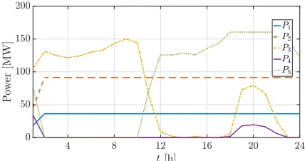
Fig. 2: Load, solar output and net load that the hydro-solar hybrid system needs to meet.
robust optimisation with Monte Carlo simulations; quantify the “cost” of uncertainty; and compare the results with stochastic programming.
A. System Description
The constraints of the Tana river cascade in terms of power output, live volume, head, and ramping characteristics may be found in [25] and are shown in Table I. The minimum power output, live volume, and water discharge rate for all reservoirs are zero, i.e., Pm
i = 0,v jm
i = 0, j = 1, . . . ,3, qmi = 0 for
i = 1, . . . ,5. The turbine generators efficiencies for the five dams are:η1= 0.9,η2= 0.9,η3= 0.92,η4= 0.89, andη5=
0.9. The analysis of deriving a simplified model for the Tana River Cascade system are given in [16] and summarised in Section II; here the results are given and then used to illustrate the robust optimal dispatch of a cascade hydroelectric system. For all the dams, we choose J = 3, i.e., we calculate the piecewise affine functions into three segments. For the five reservoirs we have:
h1(t) = 0.0281v11(t) + 0.0131v21(t) + 0.0084v13(t) + 25,
h2(t) = 0.3077v12(t) + 0.1351v22(t) + 0.0964v23(t) + 61,
h3(t) = 0.6349v13(t) + 0.4301v23(t) + 0.1667v33(t) + 131,
h4(t) = 0.5779v14(t) + 0.4117v24(t) + 0.2955v43(t) + 31,
h5(t) = 0.0648v15(t) + 0.0468v25(t) + 0.0398v53(t) + 134,
The units for the live volumes are in Mm3 and for the head in m. The time delays between the dams were calculated in [16] to be: Masinga-Kamburu, τ1 = 2 hours; Kamburu-Gitaru,
τ2 = 0<1 hour; Gitaru-Kindaruma, τ3 = 0 <1 hour; and
[image:8.612.325.539.612.725.2]Kindaruma-Kiambere,τ4= 4hours. In the Tana river cascade
[image:8.612.55.298.631.733.2]there are three main inflow streams; in Masinga, Kamburu and Kiambere. The remaining inflow into the dams is due to rainfall data. Kenya Electricity Generating Company (KenGen) provided hourly historical data of the power output of all the hydroelectric power output; dams head levels; and inflow data for all the hydroelectric power system from July 2015-June 2016. The starting volume constraint for each reservoir are given in Table I; there is no ending volume constraint. We assume that the cascade operates together with solar generation of70MW capacity; where the uncertainty is inserted. We use solar data from Solargis [29]. The shape of the national load duration curve of Kenya for 2011 is used to determine the load levels [37]. In order to determine PL(t)for t∈T, we need to make sure that the installed capacity of the hydroelectric power system is sufficient. Thus, we constrain the load to a maximum value of 590 MW < P5
i=1PiM. We will use the five hydroelectric power system to meet this load.
B. Uncertainty modelling
We define the operation of the Tana River cascade for a one day so that the net load is met. The net load is the difference between the actual load and the solar generation; as depicted in Fig. 2. For these inputs, each of the hydroelectric power systems participates as shown in Fig. 3 which are the outcomes of (18). More specifically, in order to achieve maximum system efficiency, the first two hydroelectric power stations work at maximum output. Next, Gitaru dam, the third system in row, is dispatched until the subsequent dams reach close to the maximum volume limit around t = 13 h. Then, the fourth and fifth dams, i.e., Kindaruma and Kiambere, are used to meet the demand. However, the actual output of the solar generation may be different that forecasted. In Fig. 4, the output of various sample paths of the solar output for forecast error up to 40% are depicted. It may be seen that the solar power output for, e.g., the peak hour varies from 20-60 MW. We run the hydroelectric power system scheduling algorithm as described in (18) for sample paths of the solar output for forecast errors10-40%. Some representative results are depicted in Fig. 6. It may be seen in Fig. 6b that for higher forecast errors the value of the objective function changes for different sample paths. To provide the reader a measure of how important it is to have even a faction of the meter difference in head levels we calculate how many days it takes to make the live volume zero with maximum turbine discharge, i.e., change the head level 26, 17, 9, 4.2, and 17 m, based on the data given in Table I. These are: 102, 9.5, 1.28, 0.43, and 45.3 days respectively. This is a result of different scheduling decisions based on the solar generation output. It is interesting to see how the dispatch framework changes if the hydro-solar hybrid system needs to be able to respond to changes in the solar output.
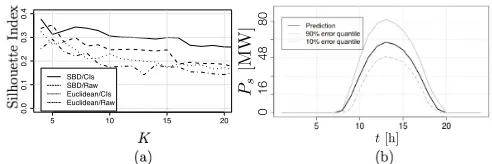
Now the solar forecasting methodology presented in Sec-tion III is illustrated. A centroid-based partiSec-tional clustering algorithm, i.e. K-means, is employed for performing clustering experiments. Fig. 5(a) depicts the Silhouette Index (one of the most efficient clustering validity index [38]) as a function of the number of clusters K, when using: the SBD distance on Clearness Indices or CIs (plain line), the SBD distance on raw data (dashed line), the Euclidean distance on CIs (dotted line) and the Euclidean distance on raw data (dash-dotted
1 4 8 12 16 20 24
[image:9.612.329.540.63.170.2]0 20 40 60 80
Fig. 4: Sample paths of solar output for a 24-hour period.
line). For each value ofK, 5 random initialisations of the K-means algorithm have been simulated (in order to avoid being trapped into a local minimum during the clustering procedure), and the solutions providing the best results for eachK have been selected to produce the plots. As observed, the best configuration (i.e. which maximises the Silhouette Index) on the whole range ofKcombines the SBD distance and the CIs. The superiority of the SBD distance over the Euclidean one is in that way clearly demonstrated in the case of the clustering of solar production patterns, regardless of the features which are used (i.e. CIs or raw data).
An example of a day-ahead prediction with its upper and lower error bounds (the 90% and 10% quantiles respectively) is also depicted on Fig. 5(b). In the present case, an optimal number of clusters of 4 has been found to provide the pre-dictions with the narrowest error bounds, which is correlated with the best Silhouette Indices obtained in Fig. 5(a). A Markov chain of order 2 has been employed: the training dataset is indeed too small to accurately identify the transition probabilities of higher order chains, even if it consists in 22 years of solar production data: for K = 4 and r = 3,
(43)2= 4096transition probabilities must be identified in the
Markov chain, out of a database made of 22×365 = 8030
objects. In fact, in the authors’ experience, it is very difficult to find larger datasets in the power system community, so that the maximum Markov chain order is practically limited to 2 in most cases with the proposed methodology. This drawback will be addressed in a future work by investigating other
0 16 48 80
Ps
[M
W
]
t[h]
5 10 15 20
0.0
0.1
0.2
0.3
0.4
K SBD/CIs SBD/Raw Euclidean/CIs Euclidean/Raw
[image:9.612.315.561.571.653.2]4 8 12 16 20 24 441
442 443 444 445 446
22 23 24
444.8 445 445.2
(a)θ= 10%.
4 8 12 16 20 24
441 442 443 444 445 446
22 23 24
444.8 445 445.2
[image:10.612.78.526.50.175.2](b)θ= 40%.
Fig. 6: Sum of head levels of the Tana River cascade for different uncertainty levels θ for a one-day period.
Machine Learning techniques to model the state transitions.
C. Influence of Uncertainty on Objective Function
In order to quantify how the uncertainty levels influence the value of the objective function, i.e., the head levels of the Tana River cascade, and the dispatch decisions we use the robust optimisation formulation presented in (22). First, we need to build a reference case against which we will be comparing the robust optimisation results. To this end, we run 500 experiments, i.e., Monte Carlo simulations, where the solar generation output period t was drawn at random, according to the uniform distribution on the segment
[(1−θ)Ps,(1 +θ)Ps] wherePs is the solar output and θ is the “uncertainty level” characteristic for the experiment. We calculate the mean and standard deviation of the objective function, i.e., P24
t=1 P5
i=1hi(t)− P24
t=1 P5
i=1M σi(t), with
M = 108. In particular, we only have P24
t=1 P5
i=1hi(t) in the objective since there is no spillage in the time period we are investigating. This mean value of the objective function for the different θ’s, when all the solar generation output were known to us in advance, is found by using (18) to determine the optimal solution and is referred to as the “ideal” case. The results of the robust optimisation reformulation could be compared with Monte Carlo simulations of the non-linear original model. However, we compared the results of the robust optimisation reformulation with Monte Carlo simulations of the approximate model, as given in (18). The approximate model differs with the original non-linear model in two elements: (i) the linearisation of the equation used to calculate the hydropower; and (ii) the relationship between the water head and the storage volume. In order to test how accurate the two approximations are and to justify the rationale
Fig. 7: Power output of Kindaruma hydroelectric plant for a day, i.e.,P4(t).
behind this choice, we calculate the difference between the power output of each hydroelectric system as the output of the optimisation problem and the actual output of each hydroelectric system calculated for a period of a whole year; the maximum error for the total power output is 3.82 MW, which is considered to be negligible. In this regard, we claim that the comparison of the robust optimisation reformulation with Monte Carlo simulations of the approximate model is meaningful due to the high accuracy and low complexity of the latter.
We solve the robust optimisation problem given in (22) to determine the influence of the solar generation uncertainty θ
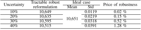
on the head levels of the Tana River cascade. To this end, we test the optimal solution of the equivalent tractable robust reformulation of (22) with the “ideal” case for uncertainty levels of10−40%. The results are summarised in Table II. As expected, the less is the uncertainty, the closer is the objective function to the ideal ones. However, we may notice that even at40% level of uncertainty the “price of robustness” is only
1.28%.
In Fig. 7 we depict the power output of Kindaruma hydro-electric plant for a one day period for various uncertainty levels
θ. As we saw in Section V-B in order to achieve maximum system efficiency, the first two hydroelectric power stations work at maximum output. Gitaru dam is dispatched until the subsequent dams reach close to the maximum volume limit around t = 13 h. Then, the fourth and fifth dams, i.e., Kindaruma and Kiambere, are used to meet the demand. However, as we see in Fig. 7 as the uncertainty level increases the participation of Kindaruma dam increases. This is a result of the affine policy rules introduced in (21) and is quantified in terms of “cost of uncertainty” in Table II.
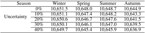
In order to assess the influence of uncertainty during differ-ent seasons we randomly select four days in the four seasons, i.e., winter, spring, summer, and autumn, and calculate the summation of the head levels of the cascade for a day-period, i.e., P24
t=1 P5
i=1hi(t), for the different seasons. The results are given in Table III. We notice that the effect of uncertainty
Uncertainty Tractable robust Ideal case Price of robustness reformulation Mean Std
10% 10,649
10,651
0.0119 0.02 %
20% 10,635 0.0219 0.15 %
30% 10,595 0.0318 0.52 %
[image:10.612.61.277.613.726.2]40% 10,515 0.0391 1.28 %
[image:10.612.316.559.673.725.2]Season Winter Spring Summer Autumn
Uncertainty
[image:11.612.56.293.51.105.2]0% 10,651.5 10,648.0 10,648.7 10,644.9 10% 10,651.1 10,647.4 10,648.2 10,643.3 20% 10,650.6 10,646.7 10,647.6 10,641.5 30% 10,650.1 10,646.1 10,647.0 10,639.5 40% 10,649.7 10,645.4 10,645.9 10,636.9
TABLE III: Head levels from tractable robust reformulation for various uncertainty level for different seasons.
is higher in the summer months as expected.
D. Comparison with Stochastic Programming
Another methodology vastly used to incorporate uncertainty in optimisation problems is with stochastic programming (see, e.g., [27]); thus it is interesting to compare the results of the proposed methodology with the aforementioned. In this regard, we model the net load at timet as a stochastic process which is represented by ∆PL(t, ω(t)), ω(t) = 1, . . . , NΩ(t); where
ω(t) is the scenario index,NΩ(t)is the number of scenarios
considered, andΩ(t)is the set of scenarios at timet. To ease notation, we assume that the number of scenarios is the same for every time t; thus ω(t)is no longer time dependent and may be denoted simply as ω = 1, . . . , NΩ. We denote by
∆PL(t)Ω the set of possible realisations of random variable
∆PL(t), i.e., ∆PL(t)Ω = {∆PL(t,1), . . . ,∆PL(t, NΩ)}.
Each realisation ∆PL(t, ω) is associated with a probability
χ(ω, t) defined as χ(ω, t) = Prob[ω|∆PL(t) = ∆PL(t, ω)],
where P
ω∈Ωχ(ω, t) = 1 for all t. The resulting two-stage
stochastic program is:
max
hi(t),Pi(t,ω),σi(t),
qi(t),vij(t)
X
t∈T X
i∈H
hi(t)−
X
t∈T X
i∈H
M σi(t)
subject to (3)−(4),(11)−(17)
X
i∈H
Pi(t, ω) = ∆PL(t, ω),∀t∈T,
ω∈Ω,
Pi(t, ω)≥νi(qmi hi(t) +hmi qi(t)−hmi qim),
∀i∈H, t∈T, ω∈Ω,
Pi(t, ω)≥νi(qMi hi(t) +hMi qi(t)−hMi qiM),
∀i∈H, t∈T, ω∈Ω,
Pi(t, ω)≤νi(qmi hi(t) +hMi qi(t)−hMi qim),
∀i∈H, t∈T, ω∈Ω,
Pi(t, ω)≤νi(qMi hi(t) +hmi qi(t)−hmi qiM),
∀i∈H, t∈T, ω∈Ω, Pm
i ≤Pi(t, ω)≤PiM,∀t∈T, i∈H,
ω∈Ω. (31)
In this two-stage stochastic linear programming problem, with first stage decisions hi(t), σi(t), qi(t), vij(t)and second stage decisions Pi(t, ω), it is possible to reduce a large scenario set to a simpler one by using the Kantorovich distance. In this case study we use fast forward selection and reduce the number of scenarios to build the set of selected scenarios
ΩS. We then use this reduced set of scenarios, i.e., replace
Ω with ΩS, in (31). Here we select 200 for the number
of reduced scenarios ΩS for every t from a pool of 500 scenarios with uncertainty 10%. The result of the two-stage stochastic program is P24
t=1 P5
i=1hi(t) = 10,651.48 m for a winter day. We compare this result with the result of the robust optimisation for 10% uncertainty for a winter day as given in Table III, i.e., 10,651.1 m. As expected the result of the robust optimisation is more conservative, than the stochastic programming result; while further reduction the number of scenarios can only improve the value of the objective function. However, the probability of a realisation of ∆PL(t),t= 1, . . . ,24occurring that will violate the con-straints is higher. Whereas with the use of linear decision rules
Pi(t) = Pid(t) +ai(t)δ(t) how much each dam participates in the net load is know before hand thus offering a policy that could be deployed in real time upon measurement of the realisation of the uncertainty without the need of solving a new optimisation program [39]. A nice extension of this work would be to use the scenario reduction heuristic of [27] for the forecast methodology and the calculation of the error. This is not the case for stochastic programming where the values of the second stage decisions, i.e.,Pi(t), are not known until the actual realisation of the uncertainty; to incorporate the latter a new optimisation problem needs to be solved. A nice extension of this work would be to use the scenario reduction heuristic of [27] for the forecast methodology and the calculation of the error.
VI. CONCLUDINGREMARKS
In this paper, we addressed the question of maximising the energy per cubic meter of water in the cascade hydroelectric system, by an optimal dispatch scheme, taking into account uncertainty from renewable-based generation coupled with the cascade, i.e., a hybrid system. In order to incorporate the uncertainty sources from renewable-based generation we develop correlated probabilistic forecasts; we use historical data and based on clustering and Markov chain techniques we determine the probabilistic forecasts. This advanced forecast technique that predicts the output of renewable resources helps in power system operations. Especially, these probabilistic predictions are useful since they may be used as input to decision making processes under uncertainty. We incorporated the aforementioned uncertainty into a robust variant of the hydroelectric dispatch problem. We used tools from robust optimisation to reformulate the original intractable problem to an amenable form while preserving immunisation against uncertainty.
In the case study, we demonstrated the robust optimal dis-patch of a cascade hydroelectric system with the hydroelectric plants of the Tana river in Kenya, which consists of five hydroelectric power plants from Masinga Main Reservoir to Kiambere and showed how the forecasting algorithm works, validated the results of the robust optimisation with Monte Carlo simulations; and quantified the “cost” of uncertainty. As expected, the less is the uncertainty, the less the cost of robustness to the objective function is. However, we may notice that even at 40% level of uncertainty the “price of robustness” is only 1.28%.
ACKNOWLEDGMENT
and support in making this work possible. The work of the authors was supported in part by the FCO under project PPF AFR 160011 and the Oxford Martin School programme of Integrating Large-scale Renewables for a Secure, Affordable and Sustainable Energy Future.
REFERENCES
[1] “Economic benefits of increasing electric grid resilience to weather outages,” Executive Office of the President, The White House, Tech. Rep., 2013.
[2] D. Apostolopoulou, A. D. Dom´ınguez-Garc´ıa, and P. W. Sauer, “An assessment of the impact of uncertainty on automatic generation control systems,”IEEE Transactions on Power Systems, vol. 31, no. 4, pp. 2657– 2665, Jul. 2016.
[3] R. H. Inman, H. T. Pedro, and C. F. Coimbra, “Solar forecasting methods for renewable energy integration,”Progress in Energy and Combustion
Science, vol. 39, no. 6, pp. 535–576, 2013.
[4] F. Golestaneh, P. Pinson, and H. B. Gooi, “Very short-term nonpara-metric probabilistic forecasting of renewable energy generation – with application to solar energy,” IEEE Transactions on Power Systems, vol. 31, no. 5, pp. 3850–3863, Sep. 2016.
[5] G. Giebel, P. Sorensen, and H. Holttinen, “Forecast error of aggregated wind power,” Tradewind, Tech. Rep., 2007.
[6] D. Lew, D. Piwko, N. Miller, G. Jordan, K. Clark, and L. Freeman, “How do high levels of wind and solar impact the grid? the western wind and solar integration study,” National Renewable Energy Laboratory, Tech. Rep., 2010.
[7] M. B. Shadmand and R. S. Balog, “Multi-objective optimization and design of photovoltaic-wind hybrid system for community smart dc microgrid,”IEEE Transactions on Smart Grid, vol. 5, no. 5, pp. 2635– 2643, Sep. 2014.
[8] P. Karampelas and L. Ekonomou, Electricity Distribution: Intelligent
Solutions for Electricity Transmission and Distribution Networks, ser.
Energy Systems. Springer Berlin Heidelberg, 2016.
[9] D. Apostolopoulou and M. McCulloch, “Optimal short-term operation of a cascade hydro-solar hybrid system,”under review in IEEE
Trans-actions on Sustainable Energy.
[10] S. V. Papaefthymiou, E. G. Karamanou, S. A. Papathanassiou, and M. P. Papadopoulos, “A wind-hydro-pumped storage station leading to high res penetration in the autonomous island system of ikaria,”IEEE
Transactions on Sustainable Energy, vol. 1, no. 3, pp. 163–172, Oct.
2010.
[11] E. Gil, I. Aravena, and R. Cardenas, “Generation capacity expan-sion planning under hydro uncertainty using stochastic mixed integer programming and scenario reduction,” IEEE Transactions on Power
Systems, vol. 30, no. 4, pp. 1838–1847, Jul. 2015.
[12] H. I. Skjelbred, “Finding seasonal strategies for hydro reservoir schedul-ing under uncertainty,” inInternational Conference on Renewable
En-ergy Research and Applications (ICRERA), Oct. 2013, pp. 579–583.
[13] R. E. Oviedo-Sanabria and R. A. Gonzalez-Fernandez, “Short-term operation planning of the itaipu hydroelectric plant considering uncer-tainties,” inPower Systems Computation Conference (PSCC), Jun. 2016, pp. 1–6.
[14] A. Hamann, G. Hug, and S. Rosinski, “Real-time optimization of the mid-columbia hydropower system,”IEEE Transactions on Power
Systems, vol. 32, no. 1, pp. 157–165, Jan. 2017.
[15] H. Dashti, A. J. Conejo, R. Jiang, and J. Wang, “Weekly two-stage robust generation scheduling for hydrothermal power systems,”IEEE
Transactions on Power Systems, vol. 31, no. 6, pp. 4554–4564, Nov.
2016.
[16] D. Apostolopoulou and M. McCulloch, “Hydroelectric power system model and its application to an optimal dispatch design,” inIREP’ 2017
- 10th Bulk Power Systems Dynamics and Control Symposium, Aug.
2017, pp. 1–6.
[17] A. J. Wood and B. F. Wollenberg,Power Generation, Operation, and
Control, ser. A Wiley-Interscience publication. Wiley, 1996.
[18] M. Cordova, E. Finardi, F. Ribas, V. de Matos, and M. Scuzziato, “Performance evaluation and energy production optimization in the real-time operation of hydropower plants,”Electric Power Systems Research, vol. 116, pp. 201 – 207, 2014.
[19] A. L. Diniz and M. E. P. Maceira, “A four-dimensional model of hydro generation for the short-term hydrothermal dispatch problem considering head and spillage effects,”IEEE Transactions on Power Systems, vol. 23, no. 3, pp. 1298–1308, Aug. 2008.
[20] Y. Zhu, J. Jian, J. Wu, and L. Yang, “Global optimization of non-convex hydro-thermal coordination based on semidefinite programming,”IEEE
Transactions on Power Systems, vol. 28, no. 4, pp. 3720–3728, Nov.
2013.
[21] J. W. Labadie, “Optimal operation of multireservoir systems: State-of-the-art review,”Journal of Water Resources Planning and Management, vol. 130, no. 2, pp. 93–111, 2004.
[22] B. Gatner and J. Matousek,Approximation Algorithms and Semidefinite
Programming. Springer-Verlag Berlin Heidelberg, 2012.
[23] F. A. Al-Khayyal and J. E. Falk, “Jointly constrained biconvex program-ming,”Mathematics of Operations Research, vol. 8, no. 2, pp. 273–286, 1983.
[24] M. Mbuthia, “Hydroelectric system modelling for cascaded reservoir-type power stations in the lower tana river (seven forks scheme) in kenya,” in3rd AFRICON Conference, Sep. 1992, pp. 413–416. [25] “Development of a power generation and transmission master plan,
kenya,” Ministry of Energy and Petroleum, Republic of Kenya, Tech. Rep., May 2016.
[26] “Integer programming,” Massachusetts Institute of Technology, Tech. Rep.
[27] A. Conejo, M. Carrion, and J. Morales, Decision making under
un-certainty in electricity markets, 1st ed., ser. International Series in
Operations Research and Management Science. Springer US, 2010, vol. 153.
[28] J. Paparrizos and L. Gravano, “k-Shape: Efficient and accurate clustering of time series,”SIGMOD Rec., vol. 45, no. 1, pp. 69–76, Jun. 2016.
[29] (2017, Mar.). [Online]. Available:
http://solargis.com/products/pvplanner/overview/
[30] X. Wang, A. Mueen, H. Ding, G. Trajcevski, P. Scheuermann, and E. Keogh, “Experimental comparison of representation methods and distance measures for time series data,”Data Mining and Knowledge
Discovery, vol. 26, no. 2, pp. 275–309, 2013.
[31] C. S. Lai, Y. Jia, M. D. McCulloch, and Z. Xu, “Daily clearness index profiles cluster analysis for photovoltaic system,” To appear in IEEE
Transactions on Industrial Informatics, 2017.
[32] W.-K. Ching, M. K. Ng, and E. S. Fung, “High order multivariate markov chains and their applications,” Linear Algebra and its
Appli-cations, vol. 428, pp. 492–507, 2008.
[33] K. Margellos and S. Oren, “Capacity controlled demand side man-agement: A stochastic pricing analysis,” IEEE Transactions on Power
Systems, vol. 31, no. 1, pp. 706–717, Jan. 2016.
[34] J. Warrington, P. Goulart, S. Mariethoz, and M. Morari, “Policy-based reserves for power systems,” IEEE Transactions on Power Systems, vol. 28, no. 4, pp. 4427–4437, Nov. 2013.
[35] D. Bertsimas and M. Sim, “Tractable approximations to robust conic optimization problems,” Mathematical Programming, vol. 107, no. 1, pp. 5–36, 2006.
[36] A. Ben-Tal, A. Goryashko, E. Guslitzer, and A. Nemirovski, “Adjustable robust solutions of uncertain linear programs,”Mathematical Program-ming, vol. 99, no. 2, pp. 351–376, Mar. 2004.
[37] “Power sector medium term plan 2015-2020,” Energy Regulatory Com-mission, Tech. Rep., 2015.
[38] O. Arbelaitzet al., “An extensive comparative study of cluster validity indices,”Pattern Recognition, vol. 46, pp. 243–256, 2013.
[39] D. Bertsimas and C. Caramanis, “Finite adaptability in multistage linear optimization,”IEEE Transactions on Automatic Control, vol. 55, no. 12, pp. 2751–2766, Dec 2010.
Zacharie De Gr`eveholds an Electrical and Elec-tronics Engineering degree from the Faculty of En-gineering of Mons, Belgium (2007). He has been a research fellow of the Belgian Fund for Research (F.R.S/FNRS) until 2012, when he got the PhD degree in Electrical Engineering, from the University of Mons. He is now a research and teaching assistant at the Electrical Power Department of the same university. His research effort is mainly dedicated to the development of Machine Learning approaches to support decision making in modern electrical power networks with a high share of renewables. He also conducts research in the field of computational electromagnetics, particularly at intermediate frequencies.