A novel wavelet selection scheme for partial discharge signal detection under low SNR condition

A Novel Wavelet Selection Scheme for Partial

Discharge Signal Detection under Low SNR Condition

Jiajia Liu1*_{, W.H. Siew}1_{, J.J. Soraghan}1_{, Xiao Hu}2_{, Xiaosheng Peng}3_{, and} Euan A. Morris1

1 _{Department of Electronics and Electrical Engineering, University of Strathclyde, Glasgow, G1 1XW, UK} 2 _{Department of Electrical Engineering, Guizhou University, Guiyang, 550025, China}

3 _{School of Electrical and Electronic Engineering, Huazhong University of Science and Technology, Wuhan,}

430074, China

*E-mail: [email protected]

Abstract:Wavelet-based techniques have been widely used to extract partial discharge (PD) signals from noisy signals. Generally, the procedure consists of 3 steps: wavelet selection, decomposition scale determination, and noise estimation. Wavelet selection is the first and most important step for its successful application in PD denoising. However, despite many variants of techniques deployed, the success rate is not generally good especially when the signal to noise ratio is unity or less. This paper discusses a novel technique that addresses this issue. The technique is inspired by the concept of Shannon entropy and the associated information cost functions (ICF) in information theory. It is adaptive to the detected PD signals. The paper demonstrates that the proposed technique is effective when applied to PD signals obtained through laboratory experiments and on-site measurements. When this technique is applied to cable diagnostics, it should have the potential to extend the range of PD detection from cables.

Index Terms:Denoising, detection, partial discharge, wavelet selection, wavelet entropy

1. Introduction

Partial discharge (PD) measurement is an effective technique for the monitoring of electrical insulation. However, PD signals are normally contaminated by noise from the environment, which increases the difficulty of their detection. To effectively extract PD signal from noisy signals, various denoising techniques, such as adaptive filter [1], [2], and the wavelet-based technique [3]–[7], have been adopted to remove noise. The wavelet-based technique has been widely used in recent years since wavelet transform can simultaneously provide signal information both in time and frequency domains. This advantage is particularly useful for the processing of non-stationary signals, e.g., PD signals.

is determined by three aspects: the choice of wavelet, decomposition scale, and noise or threshold estimation. The choice of a suitable wavelet basis function is the first, and most, significant step for the application of wavelet-based denoising as the wavelet can be translated and scaled to represent the signal of interest as effectively as possible. In practice, different denoised signals are obtained by using different wavelet basis functions [8]. This technique is also applied to the field of wavelet-based PD denoising. As such, the investigation of an appropriate wavelet basis function for wavelet-based PD denoising has been performed in [9], [10].

A wavelet selection scheme was introduced in [9] based on the correlation coefficient between a

known PD signal and wavelet waveform. This scheme is termed correlation-based wavelet selection

scheme (CBWSS). The optimal wavelet is desired to generate the highest wavelet coefficients in wavelet

analysis of PD signals, and thus, the essence of PD signal of interest can be effectively preserved. Based

on this, the wavelet that can maximize the correlation coefficient is selected as the most appropriate

wavelet for PD denoising. This approach for best wavelet selection, however, has an inherent limitation,

it requires prior knowledge of PD waveforms. The waveform of PD signals depends on: the type and

location of PD sources, propagating medium and path, and the detecting circuit. The variability of PD

waveforms impedes the application of CBWSS for online PD monitoring systems. Also, it is not a

scale-dependent wavelet selection scheme. The denoised PD signal may not be as good as expected. The most

significant drawback, however, is that the PD signal is normally corrupted by the noise in the

environment, which can lead to the selected wavelet being a match of the noisy PD signal rather than the

pure PD signal, especially when the signal to noise ratio (SNR) is very low. In an attempt to overcome

the limitation mentioned above in CBWSS, a scale-dependent energy-based wavelet selection scheme

(EBWSS) was presented in [10]. The wavelet that can maximize the energy ratio of approximation

coefficients at each decomposition scale is selected as the best wavelet. It has been demonstrated to

outperform CBWSS [10]. In EBWSS, two typical PD waveforms, damped exponential PD pulse (DEP)

and damped oscillating PD pulse (DOP), were used to demonstrate the energy criterion for the optimal

wavelet selection. With further exploration in details of EBWSS, it has been found that the criterion is

not strictly true for DOP signals, particularly when the decomposition scale increases. The motivation of

this paper is therefore to provide an automated and data-driven selection scheme for the best wavelet

selection in the context of PD denoising.

In this paper, the new wavelet selection scheme is inspired by the concept of Shannon Entropy [11],

and the associated information cost functions (ICF) in information theory [12]–[14]. An ICF can select

the best wavelet to expand a signal in wavelet domain. Wavelet entropy, derived from Shannon Entropy,

can measure the randomness of the wavelet coefficients at each decomposition scale. The smaller the

wavelet entropy, the lower the randomness of the wavelet coefficients. As such, the new selection scheme

is proposed with the combination of ICF and wavelet entropy, and termed wavelet entropy-based wavelet

selection scheme (WEBWSS). Simulated PD signals, i.e., DEP and DOP, PD signals obtained through

laboratory experiment using test samples with artificial defects and on-site PD measurements are used to

demonstrate the performance of this novel wavelet selection scheme. Results show that it is a promising

2. Wavelet-Based Technique

2.1 Wavelet Theory

Wavelet transform (WT) is an alternative approach to traditional methods, e.g. Fourier Transform, in signal processing. The major advantage of WT is that it can map a signal in the time-frequency plane. Due to this advantage, WT is a promising technique in the analysis of variations in signals or images with the requirements of both time and frequency information. WT can be interpreted as an expansion or decomposition of signals or images in terms of a wavelet that can be scaled in an auto-similar way [15]. The orthogonal property of the wavelet used for the expansion or decomposition is the essence in WT. Generally, WT is achieved through the application of continuous wavelet transform (CWT) or discrete wavelet transform (DWT). DWT is preferable due to its representation of signals or images through its DWT coefficients without redundancy and, thus, is using less computational time. In this paper, the wavelet-based technique referred to is the DWT.

In [15], the wavelet expansion of a signal x can be expressed as

𝑥 = ∑ ∑ 𝐶𝑗,𝑖∙ 𝜓𝑗,𝑖 , 𝑗

𝑖

(1)

where both i and j are integer, i is the time-delay index and j is the scale index. {𝜓𝑗,𝑖} is the expansion

set of wavelet basis functions, and {𝐶𝑗,𝑖} is the set of expansion coefficients, or wavelet coefficients,

which is called the discrete wavelet transform of x. The expansion in (1) is the inverse discrete wavelet

transform (IDWT). The scheme of DWT for signal decomposition is depicted in Figure 1. A signal is convolved with the low- and high-pass filters and followed by a downsampling operation by 2. In signal processing terminology, the outputs of the low- and high-pass filters are termed approximation and detail coefficient respectively. The approximation coefficient is used as the input signal for next-scale

decomposition. This decomposition is iterated until the predefined scale, 𝐽, reaches. It is important to

note that the maximum decomposition scale 𝐽𝑚𝑎𝑥 is defined as log2(N), where N is the length of the

input signal. The reconstruction of the input signal, i.e., inverse DWT (IDWT), is a reverse operation as shown in Figure 1. Instead of downsampling in DWT, upsampling is involved in IDWT. Figure 2 shows the processes of IDWT for signal reconstruction. To obtain perfect signal reconstruction, the low- and high-pass filters are designed as quadrature mirror filters (QMFs).

PLACE FIGURE 1 HERE PLACE FIGURE 2 HERE

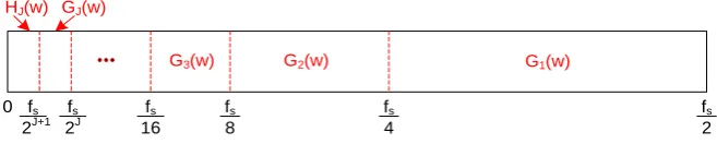
Equally, the implementation of DWT in signal decomposition also can be interpreted in the frequency domain. As shown in Figure 1, the DWT process is equivalent to filtering the signal by the filter pairs, the low-pass filter h and the high-pass filter g. Ideally, these filter pairs halve the frequency band with the increase of scale. Let fs be the sampling frequency of the input signal, the frequency band, G1(w), of the output of the high-pass filter is fs/4 ~ fs/2, while the frequency band, H1(w), of the output of the low-pass filter is 0 ~ fs/4. For next scale, H1(w) is further split into G2(w) and H2(w), which are fs/8 ~ fs/4 and 0 ~ fs/8, respectively. The frequency band is iteratively halved in the subsequent decomposition in the same manner until the predefined scale

be seen that the frequency band of low-pass filter is 0 ~ fs/2J+1 and the frequency band of high-pass filters is

fs/2J+1 ~ fs/2 for a full-scale decomposition.

PLACE FIGURE 3 HERE

2.2 Wavelet-based Denoising

The wavelet denoising theory is dependent on the fundamental idea that the energy of a signal is often concentrated in only a few coefficients while the energy of noise is widely spread among all the coefficients in the wavelet domain [9], [16], [17]. General procedures for the wavelet-based denoising of a signal are presented as follows:

1) Apply DWT to decompose the noisy signal s with a selected wavelet to a predefined scale J, and obtain

approximation coefficients 𝑎_𝐽 at the final scale J and detail coefficients 𝑑_𝑗 at decomposition scale j,

where j = 1, 2, ..., J.

2) Estimate the threshold through a noise estimation technique and apply this threshold to detail coefficients,

𝑑𝑗, at decomposition scale j using hard or soft thresholding scheme.

3) Apply IDWT to the approximation coefficients 𝑎𝐽 and the processed detail coefficients 𝑑𝑗′ to

reconstruct the denoised signal 𝑠′.

Based on the noise estimation technique proposed in [9], [18], the scale-dependent threshold used in this paper is estimated by

𝑡ℎ𝑟𝑗=

𝑀𝐴𝐷|𝑑𝑗|

0.6745 √2log (𝑛𝑗) , (2)

where 𝑀𝐴𝐷|∙| is the median absolute deviation of the detail coefficients 𝑑𝑗 at decomposition scale j, and

𝑛𝑗 is the length of 𝑑𝑗. For the thresholding scheme, soft thresholding in [18] is used in this paper, the function

is given by

𝑑𝑗,𝑖′ = {

𝑠𝑔𝑛(𝑑𝑗,𝑖)(|𝑑𝑗,𝑖| − 𝑡ℎ𝑟𝑗) 𝑖𝑓 |𝑑𝑗,𝑖| > 𝑡ℎ𝑟𝑗

0 𝑖𝑓 |𝑑𝑗,𝑖| ≤ 𝑡ℎ𝑟𝑗

, (3)

where 𝑖 = 1,2, … , 𝑛𝑗.

2.3 Wavelet Entropy

The concept of wavelet entropy was derived from Shannon entropy and presented in [19]. Suppose {𝐶𝑗,𝑖}

are the wavelet coefficients obtained through a J-scale wavelet transform, in which j represents the decomposition scale and 𝑗 = 1, 2, … , 𝐽, i denotes the ith _{element in 𝐶}

𝑗,𝑖 and 𝑖 = 1, 2, … , 𝑛𝑗, 𝑛𝑗is the length

of wavelet coefficients at scale j. The energy of wavelet coefficients at the decomposition scale j can be calculated by

𝐸𝑗= ∑|𝐶𝑗,𝑖| 2

𝑖

. ₍₄₎

The distribution of energy probability for wavelet coefficients at scale j can be derived by

𝑝𝑖=

|𝐶𝑗,𝑖| 2

∑ |𝐶𝑘 𝑗,𝑖|2

= |𝐶𝑗,𝑖|

2

𝐸𝑗 (5)

𝑊𝐸(𝑗) = − ∑ 𝑝𝑖ln(𝑝𝑖) 𝑖

. ₍₆₎

Similar to Shannon entropy, wavelet entropy is applied to measure the degree of disorder of wavelet coefficients or signify the randomness of wavelet coefficients. It is important to note that wavelet entropy is not an information cost function (ICF), since it requires the energy of wavelet coefficients to be normalized as shown in (5), and is thus not additive [13], [14]. Substituting (5) into (6) yields:

𝑊𝐸(𝑗) = ∑ 𝑝𝑖ln (

1 𝑝𝑖) 𝑖

= ∑|𝐶𝑗,𝑖|

2

𝐸𝑗 ln

𝐸𝑗

|𝐶𝑗,𝑖| 2 𝑖

= 1

𝐸𝑗 (∑|𝐶𝑗,𝑖| 2

ln 𝐸𝑗+ ∑|𝐶𝑗,𝑖| 2

𝑖

ln 1 |𝐶𝑗,𝑖|

2 𝑖

)

= ln 𝐸𝑗+

1

𝐸𝑗 (∑|𝐶𝑗,𝑖| 2

𝑖

ln 1 |𝐶𝑗,𝑖|

2

⏞ 𝑙 )

= ln 𝐸𝑗+ 𝑙 𝐸⁄ ._𝑗 (7)

In (7), 𝑙 is an ICF based on the definition in [13]. As such, wavelet entropy is a monotonic-increasing function

of 𝑙, which means minimizing 𝑙 over wavelet coefficients minimizes wavelet entropy.

3. Partial Discharge Signals

Two theoretical PD pulses, i.e., damped exponential PD pulse (DEP) and damped oscillating PD pulse

(DOP), are simulated using their mathematical frames derived based on two different PD detecting circuits

[4], [10]. In this paper, DEP and DOP are given by the formula in [10]:

𝑠1(𝑡) = 𝐴(𝑒−𝛼1𝑡− 𝑒−𝛼2𝑡), (8)

𝑠2(𝑡) = 𝐴(𝑒−𝛼1𝑡𝑐𝑜𝑠(𝑤𝑑𝑡 − 𝜑) − 𝑒−𝛼2𝑡𝑐𝑜𝑠𝜑), (9)

where 𝑠₁(𝑡) and 𝑠₂(𝑡) are the DEP and DOP respectively. The values of 𝐴, 𝛼₁, 𝛼₂, 𝑓_𝑑, 𝑤_𝑑 and 𝜑

used in these two equations are listed in Table 1.

PLACE TABLE 1 HERE

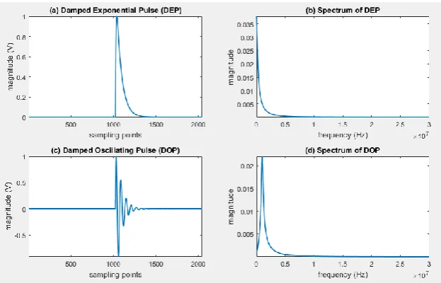
The simulated sampling frequency 𝑓_𝑠 is set to 60𝑀𝐻𝑧. Figure 4 shows these two simulated PD signals both

in time and frequency domains. Generally, DOP signal shown in Figure 4 (c) and (d) is closer to a real

high-frequency PD signal detected from electrical power equipment in practice [10].

To develop the new scheme for practical use, real PD signals were generated through an artificial defect of

a 7𝑚𝑚 × 7𝑚𝑚 breach in the outer conductor created in a 1.5m 11 kV ethylene propylene rubber-insulated

(EPR) cable sample [20]. PD signals were collected using a high frequency current transformer (HFCT). The

specifications of the HFCT are listed in Table 2. Details regarding the experiment setup are depicted in Figure

5 [20].

PLACE FIGURE 5 HERE

Experiments were performed at various voltage levels. The PD pulses measured at 9kV are used as the real

PD signals to demonstrate the new wavelet selection scheme in this paper. One PD pulse, named 𝑠₃, with

2048 sample points was selected and depicted in Figure 6.

PLACE FIGURE 6 HERE

4. Wavelet Selection Schemes (WSS)

4.1 Correlation-based Wavelet Selection Scheme

In signal processing, correlation is a measure of association between two signals, and most commonly used is the linear correlation coefficient. For two signals, 𝑥𝑖 and 𝑦𝑖, 𝑖 = 1,2, … , 𝑁, the normalized correlation

coefficient γ is given by [9]

𝛾 = ∑ (𝑥𝑖 𝑖− 𝑥̅)(𝑦𝑖− 𝑦̅) √∑ (𝑥𝑖 𝑖− 𝑥̅)2∙ √∑ (𝑦𝑖 𝑖− 𝑦̅)2

, (10)

where 𝑥̅ is the mean of xi and 𝑦̅ is the mean of 𝑦𝑖. The value of γ is in the range of -1 to 1. It takes on a

value close to 1 indicating 𝑥𝑖 and 𝑦𝑖 are positively correlated, and a value close to -1 denoting they are

negatively correlated. A value of γ near zero means 𝑥𝑖 and 𝑦𝑖 are uncorrelated.

For CBWSS [9], correlation is used as a measure of the similarity between a pure PD signal and a wavelet,

and this similarity is referred to as their shapes. The more similar their shapes, the higher the correlation

coefficient is. The wavelet that has the highest correlation coefficient with the shape of a PD signal is selected

to maximize the wavelet coefficients through wavelet analysis.

The general process for the choice of appropriate wavelet using CBWSS is described as follows:

a. Analyze the detected PD signal to generate a ‘typical’ PD pulse.

b. Set up a wavelet library, consisting of the wavelets that have similar characteristics to the PD pulse.

c. Normalize the PD pulse and each wavelet retrieved from the wavelet library.

d. Calculate the correlation coefficient, 𝛾, between the PD pulse and each wavelet.

e. Select the wavelet that has the maximum correlation coefficient with the PD pulse, it will be applied

for the following wavelet-based denoising.

As indicated in Section 1 the CBWSS approach is limited by noise and is scale-independent. Also, a heuristic method was introduced in [10] to obtain better correlation results. Resampling both the PD signal and wavelet function in time domain is applied to align their peaks as well as their first zero-crossing points after the peaks. This method is also adopted in this paper for comparisons of denoising results between EBWSS and WEBWSS methods.

4.2 Energy-based Wavelet Selection Scheme

EBWSS was proposed by Li [10], in which the wavelet that can maximize the energy ratio of the

approximation coefficients is selected as the best wavelet for PD denoising. For a one-dimensional wavelet

𝐸𝑎=

∑ 𝑎𝑖 𝑗,𝑖2

∑ 𝑎𝑖 𝑗,𝑖2+ ∑ ∑ 𝑑𝑗 𝑖 𝑗,𝑖2

, (11)

where 𝑖 = 1,2, … , 𝑛𝑖, 𝑛𝑖 is the length of approximation coefficients or detail coefficients at scale j, and dj is the detail coefficients at scale j.

The idea of wavelet energy was introduced in EBWSS. For an orthogonal wavelet, energy preservation is

one of the desirable properties of DWT [21]. The equation for energy preservation is given by

‖𝑋‖2_{= ‖𝑎‖}2_{+ ‖𝑑‖}2 _{, (12)}

where 𝑎 and 𝑑 are the approximation and detail coefficients of the DWT of a signal 𝑋. This property is also

applied to PD signals using DWT decomposition. A PD signal 𝑠 can be decomposed into 𝐽 scales with 𝐽 +

1signals, i.e., 𝑠1, 𝑠2, … , 𝑠𝐽, 𝑠𝐽+1. Among these signals, 𝑠1, 𝑠2, … , 𝑠𝐽 are detail coefficients from scale 1 to

scale 𝐽, while 𝑠_𝐽+1 is the approximation coefficients at scale 𝐽. The energy of a decomposed signal 𝑠_𝑘 is

given by

𝐸𝑘= ∑ 𝑠𝑖 𝑘2(𝑖) , (13)

where 𝑘 = 1,2, … , 𝐽 + 1, 𝑖 = 1,2, … , 𝑛𝑖, and 𝑛𝑖 is the length of 𝑠𝑖. Then, 𝑠 can be represented by a

normalized energy vector (𝑒₁, 𝑒₂, … , 𝑒_𝐽, 𝑒_𝐽+1), where 𝑒_𝑘 is defined as

𝑒𝑘=_‖𝑠‖𝐸𝑘₂= 𝐸𝑘

∑𝑘=𝐽+1𝑘=1 𝐸𝑘

. (14)

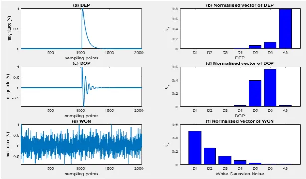
It can be seen that the concept of energy ratio in EBWSS can be interpreted as a normalized energy vector. Figure 7 shows the DEP, DOP, and white Gaussian noise (WGN) used in [10] to explain the criterion of EBWSS for wavelet selection. Figure 7 (a) and (b) show the DEP signal and its normalized energy vector respectively. Equally, Figure 7 (c) and (d) show the DOP signal and its normalized energy vector. Figure 7 (e) and (f) show WGN and its normalized energy vector. Based on Figure 7 (b), (d) and (e), the approximations of the DEP and DOP signals cover the most energy of total coefficients while the details of WGN preserve the most energy of total coefficients [10].

PLACE FIGURE 7 HERE

The general process for the choice of an appropriate wavelet using EBWSS is presented as follows: a. Given a wavelet library {𝜓𝑖: 𝑖 = 1,2, … , 𝑁} , select a wavelet from {𝜓𝑖} , and perform a one-scale

DWT decomposition of a noisy PD signal. Obtain its approximation coefficients 𝑎₁(𝑖) and detail

coefficients 𝑑1(𝑖).

b. Calculate the energy ratio of approximation coefficients 𝐸_𝑎

1(𝑖) based on (11). If 𝐸𝑎1(𝑝)is the maximum

of 𝐸_𝑎

1

(𝑖), 1 ≤ 𝑝 ≤ 𝑁, select 𝜓𝑝 as the optimal wavelet for the first scale.

c. Apply 𝜓_𝑝 to obtain the approximation coefficients 𝑎₁(𝑝) and 𝑑₁(𝑝).

d. 𝑎₁(𝑝) is used as the input signal for next-scale DWT decomposition, and select the optimal wavelet based

on the strategy used in steps a, b, and c.

e. Iterate the steps above until the predefined decomposition scale J reaches. The optimal wavelet for

each decomposition scale will be selected.

is not as robust as expected. It selects the wavelet that can maximize the energy ratio of approximation

coefficients. It is not strictly true for DOP signals, particularly when the decomposition scale increases. It can

be seen from the normalized vector of DOP in Figure 7 (d), the energy of PD signal with a 6-scale

decomposition is preserved on the detail coefficients rather than approximation coefficients. When more scales

are required, for example, 7 scales, the EBWSS is still trying to select the appropriate wavelet by maximizing

the energy ratio of approximation coefficients.

The limitation of EBWSS can be interpreted in the frequency domain. Based on Parseval’s theorem, the time and frequency domains are equivalent representations of the signal, and thus, they must have the same energy [22]. As mentioned in Section 2.1, the filter pairs of DWT iteratively halve the frequency bands of a signal with the increase of decomposition scales. The spectrum of DEP, DOP, and white Gaussian noise are illustrated in Figure 8 (a), (b), and (c) respectively. With a 6-scale decomposition, the filter pairs iteratively separate these signals into disjoint frequency bands, 𝐺1(𝑤), 𝐺2(𝑤), … , 𝐺6(𝑤) and 𝐻6(𝑤). From the

spectral curve of DOP, it is clear that the magnitudes of frequency in 𝐺5(𝑤) and 𝐺6(𝑤) are larger than those

at other frequency bands. It is in agreement with the normalized vector of DOP shown in Figure 8 (b). With further decomposition, the energy of the signal will be preserved in detail coefficients rather than approximation coefficients.

PLACE FIGURE 8 HERE

4.3 Wavelet Entropy-based Wavelet Selection Scheme

As mentioned in Section 2.3, wavelet entropy is not an ICF, but 𝑙 in (7) is monotonically increased with

the wavelet entropy. As such, the best wavelet also can be selected when the value of wavelet entropy is

minimum. In [13], it was shown that wavelet entropy value is inversely proportional to the energy concentrated

in the number of wavelet coefficients. It is also known that white noise, the noise source for PD corruption in

this paper, has high degree of randomness or disorder, and thus, the entropy value can describe the random

characters of noise [23]. Based on this, a smaller value of wavelet entropy indicates that the wavelet used for

WT decomposition can preserve more energy of the original signal in fewer number of coefficients and contain

less white noise in the wavelet coefficients and, consequently, the wavelet used is closer to the best wavelet as

expected. A new criterion for the best wavelet selection is therefore proposed, i.e., a wavelet that can have

minimum wavelet entropy of the approximation coefficients at each decomposition scale through WT

decomposition will be selected for denoising of PD detection. The new method has several promising

advantages: it is scale-dependent, automated, and data-driven.

The general process for the proposed novel wavelet selection scheme is illustrated in the flow chart in

Figure 9.

PLACE FIGURE 9 HERE

Given a wavelet library {𝜓𝑖: 𝑖 = 1,2, … , 𝑁}, one wavelet of which is selected for a one-level DWT

decomposition of a noisy PD signal s(n) each time. Next the wavelet entropy of the generated approximations

is calculated based on (6) and (7). The wavelet 𝜓𝑝 (1 ≤ 𝑝 ≤ 𝑁) that minimize the wavelet entropy of

approximations will be selected as the best wavelet. The selected 𝜓𝑝 is then applied for the DWT

𝑑1(𝑝). Finally, 𝑎1(𝑝) is used as the input signal for next scale DWT decomposition, using the strategy

presented above. When the predefined decomposition scale J reaches, the best wavelet for each scale will be

successfully selected.

5. Results and Analysis

Generally, parameters, e.g., magnitude error (ME), mean square error (MSE), signal to noise ratio (SNR),

and cross correlation (XCORR) are adopted to evaluate the performance of a proposed denoising method or

algorithm. ME, MSE, and XCORR are used in this paper to compare the denoising results of different wavelet

selection schemes. XCORR is calculated based on (11), and ME, MSE are calculated by the equations as

follows,

𝑀𝐸 = 𝑚 − 𝑚

′

𝑚 , (15)

𝑀𝑆𝐸 = ∑ [𝑠(𝑖) − 𝑠

′_(𝑖)] 𝑁

𝑖=1

𝑁 , (16)

where 𝑚 and 𝑚′ are the magnitudes of 𝑠(𝑖) and 𝑠′(𝑖) respectively. 𝑠(𝑖) represents the original signal

and 𝑠′(𝑖) denotes the denoised signal. N is the length of signals. Better denoised results can be obtained with

lower ME, MSE, and higher XCORR.

In this paper, PD signals are corrupted by white noise, and then, various wavelet selection schemes are used

to remove the noise and evaluated by the parameters mentioned above. As mentioned in Section 4.2, EBWSS

is not strictly true when the decomposition scale increases over 6. To highlight the limitations of EBWSS, the

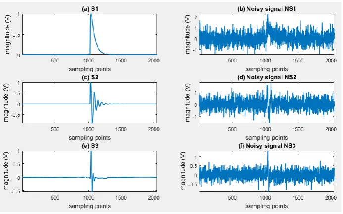
decomposition scale is set to 7 for the results analysis. Two simulated PD signals, s1 and s2, and real PD signal,

s3, as well as their noisy signals NS1, NS2 and NS3 with SNR = -10 are depicted in Figure 10. It is important to note that the original real PD signal shown in Figure 6 is corrupted by ambient noise during experiment. To

mitigate the effect of this noise on the denoising results, it has been pre-processed using the method introduced

in [10]. The smoothed real PD signal is depicted in Figure 10 (e).

PLACE FIGURE 10 HERE

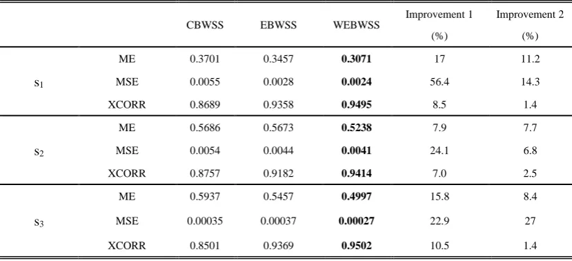
Denoised s1, s2, and s3 using CBWSS, EBWSS, and WEBWSS are shown in Figure 11 (a), (b), and (c)

respectively. The related parameters used to evaluate their performance on PD detection are listed in Table 3. It can be seen from Figure 11 and Table 3 that WEBWSS has better performance than the others of wavelet-based denoising of PD detection. Simultaneously, it also verifies the conclusion presented in [10] that EBWSS outperforms CBWSS in PD denoising.

PLACE FIGURE 11 HERE PLACE TABLE 3 HERE

Significant advancement of the proposed scheme in the denoising of single PD signals cannot be directly

seen from Figure 11. However, two columns in Table 3, Improvement 1 and Improvement 2, have presented

the improvements by WEBWSS. Improvement 1 is the improved ratio (%) of the use of WEBWSS to CBWSS

and Improvement 2 is the improved ratio (%) of the use of WEBWSS to EBWSS. From magnitude error (ME),

from these figures. The underlying meaning of the improvement of ME is PDs with small magnitude may be

picked up by the use of WEBWSS as compared to the other two schemes. This enhanced capability of PD

detection has been verified through the application of WEBWSS in on-site PD data, which will be delineated

in Figure 15. Also, the improvement of MSE and XCORR indicates that less distortion of the denoised signals

can be achieved through WEBWSS. It is good for the accuracy of PD location.

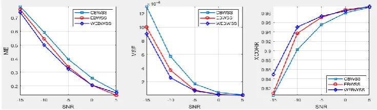
In the attempt to fully evaluate the performance of the new wavelet selection scheme, PD signals buried by

various noise levels are investigated. SNR are set to -15, -10, -5, 0, and 5 for this investigation, representing

different noise levels. The parameters used to evaluate the performance of three different schemes are plotted

in Figure 12, Figure 13, and Figure 14 for S1, S2, and S3 respectively. From the trends of ME, MSE, and XCORR for all denoised signals with the increase of SNR (the higher SNR, the lower noise level is), the new

wavelet selection scheme is better than the existing schemes for wavelet-based denoising of PD detection

under various noise levels, and the performance is particularly good when the SNR is low.

PLACE FIGURE 12 HERE PLACE FIGURE 13 HERE PLACE FIGURE 14 HERE

A PD signal is collected from one power substation in the UK with a sample rate of 100MS/s. The PD

sensor is the same type of HFCT used in laboratory in Section 3. Figure 15 delineates the original

on-site PD signal and its denoised versions by CBWSS, EBWSS, and WEBWSS, respectively. It can be

seen that not only the PD pulses with magnitudes higher than the noise level has been extracted, but those

ones with small magnitudes buried in the noise has been successfully extracted through the application

of WEBWSS in Figure 15 (d). However, the number of the PD pulses with small magnitude that have

been extracted by CBWSS and EBWSS, as shown in Figure 15 (b) and (c), is less than that by WEBWSS.

The difference of the number of small-magnitude PD extraction among these three schemes has been

highlighted in red line in Figure 15. The denoising result of on-site PD signal provides further support

that the proposed wavelet selection scheme is more advantageous than the existing EBWSS and CBWSS

for denoising of PD detection of electrical apparatus in practice.

PLACE FIGURE 15 HERE

6. Conclusion

A novel wavelet selection scheme based on the concept of information cost function and Shannon entropy

has been proposed in this paper and the results showed that the technique improved the effectiveness of

wavelet-based denoising of PD detection, especially for situations when the signal to noise ratio is unity or

less. The technique is scale-dependent, automated, and data-driven and these properties enable it to be a

promising technique in the context of PD detection. Based on the denoised results obtained from both

simulated and real PD signals, it shows better performance than the existing wavelet selection schemes,

particularly when the SNR is low. Accordingly, it has the potential to extend the range of PD detection in

References

[1] H. Borsi, “Digital location of partial discharges in HV cables,” IEEE Trans. Electr. Insul., vol.

27, no. 1, pp. 28–36, 1992.

[2] M. S. Mashikian, F. Palmieri, R. Bansal, and R. B. Northrop, “Location of partial discharges in

shielded cables in the presence of high noise,” IEEE Trans. Electr. Insul., vol. 27, no. 1, pp. 37–

43, 1992.

[3] I. Shim, J. J. Soraghan, and W. H. Siew, “Detection of PD Utilizing Digital Signal Processing

Method. Part 3 : Open-Loop Noise,” Electr. Insul. Mag. IEEE, vol. 17, pp. 6–13, 2001.

[4] X. Ma, C. Zhou, and I. J. Kemp, “Interpretation of wavelet analysis and its application in partial

discharge detection,” IEEE Trans. Dielectr. Electr. Insul., vol. 9, no. 3, pp. 446–457, 2002.

[5] L. Satish and B. Nazneen, “Wavelet-based Denoising of Partial Discharge Signals Buried in

Excessive Noise and Interference,” IEEE Trans. Dielectr. Electr. Insul., vol. 10, no. 2, pp. 354–

367, 2003.

[6] H. Zhang, T. R. Blackburn, B. T. Phung, and D. Sen, “A novel wavelet transform technique for

on-line partial discharge measurements part 1: WT de-noising algorithm,” IEEE Trans. Dielectr.

Electr. Insul., vol. 14, no. 1, pp. 3–14, 2007.

[7] P. Ray, A. K. Maitra, and A. Basuray, “Extract Partial Discharge Signal using Wavelet for

On-line Measurement,” Int. Conf. Commun. Signal Process., pp. 888–892, 2013.

[8] Y. F. Sang, D. Wang, J. C. Wu, Q. P. Zhu, and L. Wang, “The relation between periods’

identification and noises in hydrologic series data,” J. Hydrol., vol. 368, pp. 165–177, 2009.

[9] X. Ma, C. Zhou, and I. J. Kemp, “Automated wavelet selection and thresholding for PD

detection,” IEEE Electr. Insul. Mag., vol. 18, no. 2, pp. 37–47, 2002.

[10] J. Li, T. Jiang, S. Grzybowski, and C. Cheng, “Scale dependent wavelet selection for de-noising

of partial discharge detection,” IEEE Trans. Dielectr. Electr. Insul., vol. 17, no. 6, pp. 1705–

1714, 2010.

[11] C. E. Shannon, “A Mathematical Theory of Communication,” Mob. Comput. Commun. Rev., vol.

5, no. 1, 1948.

[12] R. R. Coifman and M. V. Wickerhauser, “Entropy-based algorithms for best basis selection,”

IEEE Trans. Inf. Theory, vol. 38, no. 2, pp. 713–718, 1992.

[13] M. V. Wickerhauser, Adapted Wavelet Analysis from Theory to Software, vol. 38, no. 1. IEEE

Press, 1996.

[14] H. Šikić and M. V. Wickerhauser, “Information cost functions,” Appl. Comput. Harmon. Anal.,

vol. 11, no. 2, pp. 147–166, 2001.

[15] S. Alessio, Digital Signal Processing and Spectral Analysis for Scientists: Concepts and

Applications. Springer, 2015.

[16] A. O. Boudraa, J. C. Cexus, and Z. Saidi, “EMD-based Signal Noise Reduction,” Int. J. Signal

Process, pp. 33–37, 2004.

[17] Y. Kopsinis and S. McLaughlin, “Development of EMD-Based Denoising Methods Inspired by

Wavelet Thresholding,” Signal Process. IEEE Trans., vol. 57, no. 4, pp. 1351–1362, 2009.

[18] D. L. Donoho and I. M. Johnstone, “Ideal spatial adaptation by wavelet shrinkage,” Biometrika,

vol. 81, no. 3, pp. 425–455, 1994.

[19] Y. Zhuang and J. S. Baras, “Existence and Construction of Optimal Wavelet Basis for Signal

Representation,” IEEE Trans. Signal Process., 1994.

used in partial discharge detection,” IEEE Trans. Dielectr. Electr. Insul., vol. 24, no. 2, pp. 1088– 1096, 2017.

[21] M. Misiti, Y. Misiti, G. Oppenheim, and J.-M. Poggi, Wavelet ToolboxTM _{User’s Guide. 2015.}

[22] S. W. Smith, The Scientist and Engineer’s Guide to Digital Signal Processing, Second Edi.

California Technical Publishing, 1999.

[23] Z. He, X. Chen, and G. Luo, “Wavelet Entropy Measure Definition and Its Application for

Transmission Line Fault Detection and Identification; (Part I: Definition and Methodology),”

2006 Int. Conf. Power Syst. Technol., pp. 1–6, 2006.

Jiajia Liu was born in Jiangsu, China, in 1985. He received the BSc degree in electrical engineering from Shanghai Maritime

University in 2007, the MSc degrees in electrical engineering from Shanghai Maritime University and the University of

Southampton in 2009 and 2014 respectively. He is currently pursuing his PhD degree at the University of Strathclyde. His major

research interest includes partial discharge monitoring, and transformer thermal modeling.

W. H. Siew is a Professor in the Department of Electronic & Electrical Engineering, University of Strathclyde, Glasgow, U.K. He

is a Triple Alumnus of the University of Strathclyde with the B.Sc. (Hons) degree in electronic and electrical engineering; the Ph.D.

degree in electronic and electrical engineering; and the M.B.A. degree. His areas of research interest include large systems

electromagnetic compatibility, cable diagnostics, lightning protection, and wireless sensing systems. He was the Convener of the

CIGRE WG C4.208 and of CIGRE WG C4.30. He is a member of the Advisory Group for CIGRE SC C4, which addresses

System Technical Performance of Large Electric Systems. He is a Chartered Engineer and is an MIEEE and an MIEE.

John J. Soraghan(S’83–M’84–SM’96) received the B.Eng. (Hons.) and M.Eng.Sc. degrees from University College Dublin,

Dublin, Ireland, in 1978 and 1983, respectively, and the Ph.D. degree from the University of Southampton, Southampton, U.K., in

1989, all in electronic engineering. His doctoral research focused on synthetic aperture radar processing on the distributed array

processor. After graduating, he worked with the Electricity Supply Board in Ireland and with Westinghouse Electric Corporation

in the United States. In 1986, he joined the Department of Electronic and Electrical Engineering, University of Strathclyde,

Glasgow, U.K., as a Lecturer and became a Senior Lecturer in 1990, a Reader in 2000, and a Professor in signal processing in

September 2003, within the Institute for Communications and Signal Processing (ICSP). In December 2005, he became the Head

of the ICSP. He currently holds the Texas Instruments Chair in Signal Processing with the University of Strathclyde. He was a

Manager of the Scottish Transputer Centre from 1988 to 1991 and a Manager of the DTI Parallel Signal Processing Centre from

1991 to 1995. His main research interests include signal processing theories, algorithms, and architectures with applications to

remote sensing, telecommunications, biomedicine, and condition monitoring. Prof. Soraghan is a member of the Institution of

Engineering and Technology.

Xiao Hu graduated from Xi’an Jiaotong University with a BSc degree and a MSc degree in electrical engineering in 2006 and

2009, respectively. He received his PhD degree from the University of Strathclyde in 2014 for research on FDTD modeling of

partial discharge in high voltage cables. He is currently a lecturer in Guizhou University, China and his research includes partial

discharge measurement and modeling.

Xiaosheng Peng received the B.Sc. And M.Sc. degrees from Huazhong University of Science and Technology, China in 2006 and

2009, respectively, and the Ph.D. degree in electrical engineering at Glasgow Caledonian University in 2012 funded by EPSRC.

He has worked as a Post-Doctoral Researcher in Glasgow Caledonian University funded by EDF Energy. He is currently a lecturer

in school of Electrical and Electronic Engineering of Huazhong University of Science and Technology. His research interests are

Euan A. Morris was born in Glasgow, Scotland, in 1991. He received the MEng. degree in electrical and electronic engineering

with business studies from the University of Strathclyde, Glasgow in 2014 and is currently undertaking the Ph.D. degree at the

EPSRC Centre for Doctoral Training in Future Power Networks and Smart Grids, run by the University of Strathclyde, Glasgow

and Imperial College London, London.

Input data 2 2 2 2 Low-pass filter h g h g High-pass filter Downsampling Detail cfs

Approx. cfs _{Low-pass filter}

High-pass filter

Downsampling Scale 1

Scale 2

Figure 1. The implementation of DWT in signal decomposition

2 Low-pass filter High-pass filter Upsampling Detail cfs Approx. cfs Scale 2 2 2 2 g ~ h ~ Low-pass filter High-pass filter Scale 1 g ~ h ~ Output data Upsampling

Figure 2. The implementation of IDWT in signal reconstruction

G1(w) G2(w)

G3(w) GJ(w)

HJ(w)

fs 2 fs 4 fs 8 fs 16 fs 2J fs 2J+1 0

Figure 3. The frequency bands of filters at each decomposition scale

Table 1.Values of parameters used in (8) and (9) [10].

Parameters Values

𝐴 1

𝛼1 106𝑠−1

𝛼2 107𝑠−1

𝑓𝑑 1𝑀𝐻𝑧

𝑤_𝑑 2𝜋𝑓_𝑑

𝜑 𝑡𝑎𝑛−1_(𝑤

Figure 4. (a) and (b): DEP signals simulated in time and frequency domain respectively; (c) and (d): DOP signals simulated in

time and frequency domain respectively.

Table 2.Specifications of the HFCT.

Parameters HFCT

Sensitivity 5 V/A

-3 dB bandwidth 90 kHz – 20 MHz

Internal diameter 50 mm

External diameter 110 mm

Load resistance 50 𝛺

Output conductor BNC

Manufacturer IPEC

-30 dB

+25 dB

AC Tr

Zn

Zm

Ck

Wide-band attenuator

Wide-band amplifier LeCroy 104Xi, 1GHz

HFCT

Cable sample Earth Strap

Stress cone

Artificial defect Voltage

probe

Figure 5. PD testing of a defective 11 kV EPR cable. HFCT was used to collect PD pulses (Ck and Zm represent the coupling

Figure 6. Real PD pulse, s3, detected from a defective EPR cable under 9kV AC voltage

Figure 7. Representation of (a): DEP, (c): DOP, and (e): WGN by normalized vectors (b), (d) and (f) respectively.

G1(w) G2(w)

G3(w) G4(w)

G5(w) G6(w) H6(w)

Start

Load PD signal, s(n), set Up a wavelet library, Ψi, i = 1 ,2,…,N,

and the decomposition scales, J

DWT of s(n) using Ψi for one-scale

decomposition, i = 1, j = 1

Obtain the approx. cfs, aj(i)

Calculate the energy of aj(i) and its

energy probability (equation (5))

Calculate the wavelet entropy, and store it into a entropy vector WE(i)

(equation (6))

i = N ?

No

[~,p] = min(WE(i)), p [1,N]

Ψpis selected as the optimal

wavelet for scale j and stored into an wavelet vector ow(j)

Obtain the approx. cfs aj(p)and

detail cfs dj(p) for scale j using Ψp

Store approx. & detail cfs to the vectors a and d respectively

Yes

j = J ?

Set s(n) = aj(p) for optimal wavelet

selection at next scale, j = j+1

No

Yes

End

i = i + 1

Figure 9. Flow chart of the general process of WEBWSS.

Figure 10. (a) and (b): s1 and its noisy signal NS1 with SNR = -10, (c) and (d): s2 and its noisy signal NS2 with SNR = -10, (e)

Figure 11. (a): Denoised s1 using CBWSS, EBWSS and WEBWSS, (b): Denoised s2 using CBWSS, EBWSS and WEBWSS,

(c): Denoised s3 using CBWSS, EBWSS and WEBWSS.

Table 3.Parameters used to evaluate the performance of wavelet selection schemes.

CBWSS EBWSS WEBWSS

Improvement 1

(%)

Improvement 2

(%)

s1

ME 0.3701 0.3457 0.3071 17 11.2

MSE 0.0055 0.0028 0.0024 56.4 14.3

XCORR 0.8689 0.9358 0.9495 8.5 1.4

s2

ME 0.5686 0.5673 0.5238 7.9 7.7

MSE 0.0054 0.0044 0.0041 24.1 6.8

XCORR 0.8757 0.9182 0.9414 7.0 2.5

s3

ME 0.5937 0.5457 0.4997 15.8 8.4

MSE 0.00035 0.00037 0.00027 22.9 27

Figure 12. ME, MSE and XCORR between s1 and denoised s1.

Figure 13. ME, MSE and XCORR between s2 and denoised s2.

Figure 15. The denoising results of on-site PD signal: (a) On-site detected PD signal; (b), (c), (d) are the denoised PD signal by