Benchmarks for Evaluating Optimization
Algorithms and Benchmarking MATLAB
Derivative-Free Optimizers for Practitioners’
Rapid Access
LIN LI1, (Member, IEEE), ALFREDO ALAN FLORES SALDIVAR 1, YUN BAI1, (Member, IEEE), YI CHEN 1, (Senior Member, IEEE), QUNFENG LIU 1, AND YUN LI 1,2, (Senior Member, IEEE)
1Industry 4.0 Artificial Intelligence Laboratory, Dongguan University of Technology, Dongguan 523808, China
2Department of Design, Manufacturing and Engineering Management, Faculty of Engineering, University of Strathclyde, Glasgow G1 1XJ, U.K.
Corresponding author: Yun Li ([email protected])
This work was supported in part by the Guangdong Higher Education Research Program under Grant 2017KQNCX193, in part by the Dongguan University of Technology under Research Grant ‘Industry 4.0 Smart Design and Innovation Platform’ KCYKYQD2017014 and under Postdoctoral Research Start-Up Grant GC300501-18, and in part by the National Natural Science Foundation of China under Grant 71801044 and Grant 61773119.
ABSTRACT MATLABR has built in five derivative-free optimizers (DFOs), including two direct search algorithms (simplex search, pattern search) and three heuristic algorithms (simulated annealing, particle swarm optimization, and genetic algorithm), plus a few in the official user repository, such as Powell’s conjugate (PC) direct search recommended by MathWorksR. To help a practicing engineer or scientist to choose a MATLAB DFO most suitable for their application at hand, this paper presents a set of five benchmarking criteria for optimization algorithms and then uses four widely adopted benchmark problems to evaluate the DFOs systematically. Comprehensive tests recommend that the PC be most suitable for a unimodal or relatively simple problem, whilst the genetic algorithm (with elitism in MATLAB, GAe) for a relatively complex, multimodal or unknown problem. This paper also provides an amalgamated scoring system and a decision tree for specific objectives, in addition to recommending the GAe for optimizing structures and categories as well as for offline global search together with PC for local parameter tuning or online adaptation. To verify these recommendations, all the six DFOs are further tested in a case study optimizing a popular nonlinear filter. The results corroborate the benchmarking results. It is expected that the benchmarking system would help select optimizers for practical applications.
INDEX TERMS Optimization methods, heuristic algorithms, evolutionary computation, benchmark testing, particle filters.
I. INTRODUCTION
As a high-level technical computing language and devel-opment environment, MATLABR has over 4,000,000 reg-istered users and over 525,000 contributors to its official repository [1]. It builds in five ‘derivative-free optimizers’ (DFOs) in the form of heuristic and direct search algorithms. These DFOs have provided powerful tools suitable for a broad range of real-world optimization applications and have hence been widely used by optimization practitioners [2]–[4].
The associate editor coordinating the review of this manuscript and approving it for publication was Wei Wei.
However, with the development of optimizers beyond con-ventional means, it has become challenging for a practicing engineer or scientist to select the most suitable one for their application at hand, especially without a common ground or a full set of criteria available for assessment. At present, there exists no widely applicable theoretical or analytical means to compare the performance of numerical optimizers. Further, benchmarks for comparing optimizers through tests are incomplete, mainly relying on fitness and convergence as benchmarks [5], despite a large number of benchmarking tests have been reported [6]. It is thus still difficult to assert quickly whether one particular algorithm is indeed ‘better’ or ‘more suitable’ than the others for a practitioner’s application.
VOLUME 7, 2019
2169-35362019 IEEE. Translations and content mining are permitted for academic research only.
This paper aims to help practitioners rapidly to select a numerical optimizer, and in particular a DFO, suitable for their application at hand without needing to become an expert in these algorithms first. Therefore, we establish a full set of benchmarks for comparing DFOs, extending beyond those benchmarks currently available in the literature. Further, a scoring system for benchmarking DFOs and a decision tree are to be developed to facilitate their selection and use without the need for deep knowledge of the DFOs on the user’s part. We shall carry out complete benchmark tests against four Congress on Evolution Computation (CEC) benchmarking problems [7]–[11], and then verify the conclusion against a practical application - the particle filtering (PF) problem [12]. Included in the benchmarking tests are five MATLAB built-in DFO functions [2]–[4], i.e. simulated annealing (SA), particle swarm optimization (PSO), the genetic algorithm (with elitism, GAe), simplex search (SS), and pattern search (PS), plus one third-party implementation of the widely used Powell’s conjugate (PC) method (as an open-source m-file available from MATLAB’s official user repository [13]) rec-ommended by MathWorksR [7]. Among these six DFO algorithms, the SS, PS and PC are direct search algorithms and the other three are heuristics, where the GAe uses encoding.
The following section analyzes the four CEC benchmark problems to be adopted in benchmarking. Then, Section III develops the full set of benchmarks for comparing numerical optimization algorithms. Section IV undertakes benchmark-ing tests, and then discusses the results with recommen-dations. Given the recommendations, Section V tests the DFOs further, in a case study of a nonlinear particle filter application. Section VI summarizes the paper and draws conclusions.
II. BENCHMARKING ANALYSIS FOR MATLAB DFOs
A. OPTIMIZATION OBJECTIVES AND SOLUTIONS
For evaluating the performance of optimization, search or machine learning algorithms, consider a benchmarking opti-mization problem. Suppose that the objective function or ‘performance index’ of the optimization, subject to direct and/or indirect constraints, is represented by:
f (x):X→F (1)
which is also called afitness functionin the context of max-imization, or acost function in that of minimization. Here, f ∈ F ⊆ Rm represents m objective elements, and x ∈
X⊆RDrepresentsD decision variablesor parameters to be
optimized. The benchmark functionfmay only be evaluated numerically through computer simulations withinX.
As MATLAB DFOs are usually for a single objective, which would nonetheless include all elements off through preference weighting, we consider the casem = 1 here for simplicity. For benchmark testing, a benchmark problem or test function usually has a knowntheoretical optimum:
f0=min
x∈Xf (x) (2)
Without loss of generality, minimization is typically considered, as maximization is simply an inverse case of minimization.
Note that a non-numerical decision variable, including a ‘logic’ variable (such as True/On or False/Off) and a ‘cate-gory’ variable (such as R, L or C in an electronic circuit) may only take a discrete value inR1, in the form of an encoded xas accommodated in the genetic algorithm or genetic pro-gramming. For anx0∈Xthat satisfies:
f (x0)=f0 (3) it is said to be atheoretical solutioncorresponding tof0to the optimization problem.
Letxˆ0∈ Xrepresent afound solutionby an optimization, search or machine learning algorithm, such as a DFO. Then, the correspondingfound optimumis defined as
ˆ
f0=f xˆ0 (4) which is usually an approximate optimum or a sub-optimum with respect to nondeterministic algorithms. Since DFOs are often nondeterministic, benchmarking should use mathemat-ical means of results over multiple test runs.
According to evolutionary algorithm competitions in IEEE CEC’14 and CEC’15, many real-world problems are multi-modal and can be represented by a set of benchmark problems or, analytically, test functions [8], [9]. Local optimization is concerned with unimodality, and global with multimodal-ity. Given possible modal differences in different dimen-sions, four benchmark problems of unimodal, multimodal and hybrid types are used in this paper to illustrate and analyze benchmarking with thorough comparison. Further, all the functions are tested in 10 and 30 dimensions for 30 times [8], [9].
B. UNIMODAL PROBLEM
One of the basic test functions is a unimodal function, such as the Quartic test functionf1[14], [15]:
f1(x)=
XD
i=1ix 4
i +random[0,1) (5)
wherex∈[−1.28,1.28]D, random[0, 1) is a Gaussian noise that helps assess the robustness of the tests, andf1(x) ∈ [0,147.64] andf1(x) ∈ [0,1248.2] forD=10 andD=30, respectively. A 3-D map for a 2-D function is shown in Fig. 1.
C. MULTIMODAL PROBLEMS
In addition to multidimensionality, multimodality is also a common feature seen in practical applications. Two example benchmark problems are given below.
1) VARYING LANDSCAPE MULTIMODAL PROBLEM
Consider the D-dimensional maximization problem intro-duced by Michalewicz [16] and further studied by Renders and Bersini [15]:
f2(x)=
XD
i=1fi(xi)=
XD
i=1sin(xi)sin 2m ixi2
π
!
FIGURE 1. Contour plot to visualize a 2-D case off1.
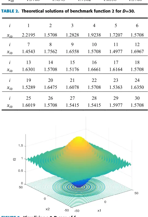
FIGURE 2. Visualizing a 2-D case off2.
where x∈[0, π]D. It is composed of a family of amplitude-modulated sinewaves whose frequencies are lin-early modulated. A 3-D map of a 2-D function is shown in Fig. 2.
The objective function f2(x) is, in effect, de-coupled in every dimension represented by fi(xi), for the ease of
ver-ifying optimality. This characteristic yields the following properties:
1) The larger the productmDis the sharper the landscape becomes, and hence harder for the optimizer.
2) There areD! =2.6525×1032local maxima within the search space [0, π]30.
3) The theoretical benchmark solution to this
D-dimensional optimization problem may be obtained by maximizingDindependent uni-dimensional func-tions, fi, ∀i ∈ {1,· · ·,D}, a fact that is however
unknown to the optimizer under test. The results for
D∈ {10,30}and form=100 aref2(x)∈[0,9.56] and
f2(x) ∈ [0,29.63], respectively. The corresponding theoretical solutions are shown in Tables 1 and 2. 4) The ease of obtaining theoretical benchmarks
regard-less ofDmakes it ideal for studying nondeterministic polynomial (NP) characteristics of the algorithms being tested.
2) EXPANDED SCHAFFER’S MULTIMODAL PROBLEM Consider a third test functionf3of the expanded Schaffer’s F6 function [8], [9], which includes many peaks and is difficult
[image:3.576.295.536.136.490.2]TABLE 1.Theoretical solutions of benchmark function 2 forD=10.
TABLE 2.Theoretical solutions of benchmark function 2 forD=30.
FIGURE 3. Visualizing a 2-D case off3.
for an algorithm to converge to:
f3(x)=g(x1,x2)+g(x2,x3)+ · · · +g(xD−1,xD)
+g(xD,x1)
g(x,y)=0.5+
sin2px2+y2−0.5
1+0.001 x2+y22 (7)
wherex∈ [−100,100]D,f3(x) ∈ [0,9.98] and f3(x) ∈ [0,29.93] forD=10 andD=30, respectively. A 3-D map for a 2-D function is shown in Fig. 3.
D. HYBRID PROBLEM
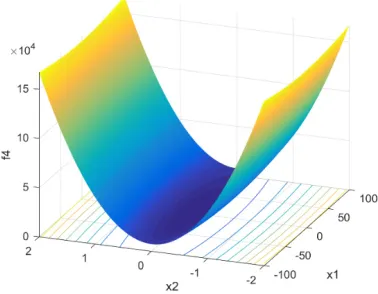
[image:3.576.67.248.222.370.2]FIGURE 4. Visualizing a 2-D case off4.
and the High Conditioned Elliptic Functionf43[8], [9]:
f4(x)=0.3f41(x)+0.3f42(x)+0.4f43(x)
f41(x)=418.9829D−
XD
i=1g(zi), (8)
zi =xi+4.209687462275036×10² (9)
g(zi)=
zisin |zi|1/2
if |zi| ≤500
(500−mod(zi,500))
×sin √|500−mod(zi,500)|
−(zi−500) 2
10000D if zi>500
(mod(|zi|,500)−500)
×sin
√
|mod(|zi|,500)−500|
−(zi+500) 2
10000D ifzi<−500
(10)
f42(x)=
XD
i=1
xi2−10cos(2πxi)+10
(11)
f43(x)=
XD
i=1
106
i−1 D−1
xi2 (12)
wherex∈[−100,100]D and the hybrid rates used are 0.3, 0.3 and 0.4 for f41(x),f42(x)andf43(x), respectively. For
D=10 and D=30,f4(x) ∈ 0,5.54×108and f4(x) ∈
0,1.22×109, respectively. The objective of this bench-mark problem is to minimizef4(x), which is like a unimodal problem as depicted in Fig. 4 whenD=2, which is relatively simple in global optimization.
In summary, f1 is unimodal for testing local DFOs, f4 is relatively simple in terms of modality, and f3 andf4 are multimodal for testing global DFOs.
III. FULL SET OF BENCHMARKS FOR EVALUATING NUMERICAL OPTIMIZERS
A. OPTIMALITY BENCHMARK
Optimalityrepresents the relative closeness of a found opti-mum, fˆ0, to the theoretical optimum, f0, which is defined
here as:
Optimality=1−
f0−
ˆ f0 f −f
∈[0,1] (13)
wheref andf are the lower and upper bounds off, respec-tively, which are known from proper benchmark problems or test functions.
For a single objective problem (i.e.m = 1), consider the minimization problem with an objective bound of [fmin,fmax] as an example. Then, by (13), the optimality benchmark can be simplified to:
Optimalitymin=1−
fmin− ˆf0
|fmax−fmin|
= fmax− ˆf0
fmax−fmin
(14)
Similarly, the optimality for the corresponding maximiza-tion problem can be simplified to:
Optimalitymax=1−
fmax− ˆf0
|fmax−fmin|
= ˆ
f0−fmin
fmax−fmin
(15)
B. ACCURACY BENCHMARK
Is it necessary to introduce an accuracy benchmark in the control space in addition to the Optimality benchmark that already reflects a ‘performance index’ in the objective space? The necessity lies in that we are assessing global optimization that involves multiple optima and is approached stochasti-cally often by a nondeterministic algorithm. As the highest value of optimality is one of the local optima, the quality of a found solutionxˆ0 obtained by an algorithm cannot be assessed by the optimality benchmark alone ifxˆ0does not lie in the neighborhood of the global optimum.
Here, theaccuracybenchmark is defined as the relative closeness of the found solution, xˆ0, to the theoretical solution,x0:
Accuracy=1−kx0−bx0k
kx−xk ∈[0,1] (16) wherex is the lower bound ofx andx is the upper bound, and
x,x
represents the search range. This benchmark may be particularly useful if the solution space is noisy, there exist multiple optima, or ‘niching’ is used.
By (16), the accuracy with respect to a single-parameter minimization problem within [xmin,xmax] is measured by:
AccuracyD=1=1− ˆ
x0−x0
xmax−xmin
(17)
C. CONVERGENCE BENCHMARKS
To date, convergence of population-based algorithms is benchmarked only qualitatively using fitness or cost traces graphically against the number of iterations, generations or function evaluations (FEs). With this paper, convergence can now be measured both qualitatively and quantitatively.
• The highest ‘optimality’ or fitness in every generation; • The highest ‘accuracy’ or the parameter values of the
individual solution that has the highest optimality fitness in every generation.
1) REACH TIME
Quantitatively, we define a ‘reach time’ as:
Reach time|b=Cb (18) where C is the count of ‘function evaluations’ performed when the optimality of the best individual first reaches a predefined valueb, whereb∈ [0,1], i.e., when the distance to the theoretical objective first drops to(1−b). For instance,
C0.999 indicates the generation number needed for an opti-mizer to reach the optimality with an error no greater than 0.1%, andC0.632indicates a convergence ‘time constant’ by which time optimality of 63.2% is first reached (in a manner similar to a first-order dynamic behavior).
2) NP-TIME
The power of a heuristic DFO is that it reduces an other-wise exponential time of an exhaustive search algorithm to a nondeterministic polynomial time. To estimate the order of the polynomial,C0.999may be plotted against the number of parameters being optimized,D. We can hence also propose a revised reach time, ofDcomponents, as:
NP−time(D)=C0.999(D) (19) 3) TOTAL NUMBER OF FUNCTION EVALUATIONS
The optimality of 99.9% may not be reached by certain algo-rithms under test. The total number of function evaluations is the number of evaluations, search trials or simulations performed until the optimization process is terminated. For benchmarking, the total number of evaluations is kept the same for all algorithms, such as 400mD2, which is more informatively defined as:
N =minnC0.999,400mD2o (20) Namely, withC0.999, the benchmark test will terminate when the goal of the optimality reaching an error no greater than 0.1% is achieved or 20Dgenerations with a population size of(20D×m)have been iterated.
D. OPTIMIZER OVERHEADS BENCHMARK
The ‘total CPU time’,Tin seconds, of the entire optimization process can also be used in a benchmark test when assessing how long an optimization process would take in the real world to single out the amount of program overheads due to opti-mization maneuvers. Quantitatively, the optimizer overheads benchmark is defined as:
Optimizer overheads= T−TFE
TFE
(21)
whereTFEis defined as the CPU time taken (in seconds) for completingN function evaluations.
E. SENSITIVITY BENCHMARK
When the values of the optimal parameters found are per-turbed, the optimality may well change, which will affect the reliability or robustness of the solution found and can hence impact on the quality of real-world applications. This is criti-cal, for example, in an industrial design, where manufacturing tolerance may cause suddenly deteriorated quality of the end product as a result of the sensitive optimality or polarized optimization.
In this paper, ‘‘sensitivity’’ is hence used to indicate the robustness of the optimizer by measuring how much relative change in the optimality will result from a ‘small’ relative change in the corresponding solution found. Quantitatively, the sensitivity is hence defined as:
Sensitivity= d(Optimality)
d(Accuracy) =
∇ ˆf
x−x
f −f
(22)
In other words, sensitivity is a scaled ‘relative gradient’, which can be estimated to:
Sensitivity≈ 1 ˆ f 1xˆ
x−x
f −f
(23)
where1ˆfis a neighborhood ofˆf0and1xˆis the correspond-ing neighborhood of the solution found.
It is convenient to set1xˆ=1%, which means that the pre-vailing sensitivity measures how many percent the optimality will degrade if the accuracy is 1%off. Note that the trend of sensitivity is rather dependent on the nature of the problem (e.g., the test function), and not mainly on the optimizer.
In addition to sensitivity, the two-tailed ‘‘t-test’’ could be used to assess the reliability in comparing two algorithms to a certain degree [14], [18]. This is a statistical hypothesis test, which is usually used to determine if two sets of data are significantly different from each other [19] and used as a complimentary approach to further validation of a compari-son when necessary.
IV. BENCHMARKING MATLAB DFOs
A. TEST CONDITIONS
Using the defined benchmarks and the chosen benchmark problems, we investigate the performance of the MATLAB (R2016b) heuristics SA, PSO and GAe, and the direct-search optimizers, SS, PS, and PC, through extensive experimental tests. Since the main purpose of this work is to help MATLAB DFO users select an algorithm without the need for in-depth knowledge of the algorithms, MATLAB’s default settings for these algorithms are used in the tests (unless otherwise stated) and all the DFOs are tested on the same random set of starting points.
Therefore, for SS, the reflection coefficient is 1, the expan-sion coefficient 2, the contraction coefficient 0.5, and the shrink coefficient 0.5.
For PSO, the swarm size is 20D, whereDis the dimension number of the test function. The maximum iteration is 20D; so the maximum number of function evaluations is 400D2.
MATLAB’s genetic algorithm uses elitism, hence named GAe, which guarantees the best 5% of a generation to survive to the next generation. For the GAe, the population size is 20D. The maximum number of generations is also 20D; so the maximum number of function evaluations is the same as PSO. The crossover rate was 0.8, and the mutation rate is 0.2. Each experiment is repeated 30 times to obtain a mean value of each benchmark value. As SA, SS, PS and PC are unary (as opposed to population-based) optimizers, one starting point is generated randomly for each run, identically used by all of these optimizers for fair comparison. Note that, however, when displaying convergence traces for these unary optimizers, one point is plotted for every 20DFEs, so as to compare fairly with one ‘generation’ of the population-based optimizers. For each run of the latter, the initial generation of 20Dindividuals are generated randomly for use identically by both PSO and the GAe.
In order to compare the optimizer overheads later, the CPU time, albeit less accurate in MATLAB than in a real-time program, is recorded forNfunction evaluations. The average
[image:6.576.317.520.63.404.2]TFE over 30 runs for every benchmark problem is shown in Table 3. It also reveals that, whenDincreases by two times from 10 to 30,TFEincreases by over 20 times, indicating a highly nonlinear challenge by the dimensionality. These FEs were performed on a PC of an Intel Core i7-4790K 4.00 GHz CPU with 8 GB RAM running a Windows 64-bit operating system.
TABLE 3. Time taken byNFEs and dimensionality challenge.
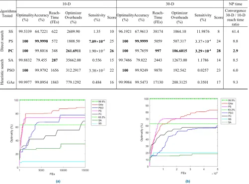
B. BENCHMARKING DFOs ON FOUR TEST PROBLEMS The performance of the six individual algorithms on each of the five benchmarks was first ranked and then assigned scores from 6 to 1, with 6 representing the best. For example, if the mean optimality of PSO is the highest among all the six algorithms, then it scores a 6 on Optimality. The scores of each algorithm on all the five benchmarks are summed up to give the algorithm a total score. Results from all the experiments are summarized in Tables 4-7, where the bold indicates the best at each benchmark and the red the best overall score and corresponding algorithm.
1) QUARTIC UNIMODAL PROBLEMf1
It can be observed that, for 10-D, the algorithms except SS and SA offer optimality over 99.9995%. PC offers the
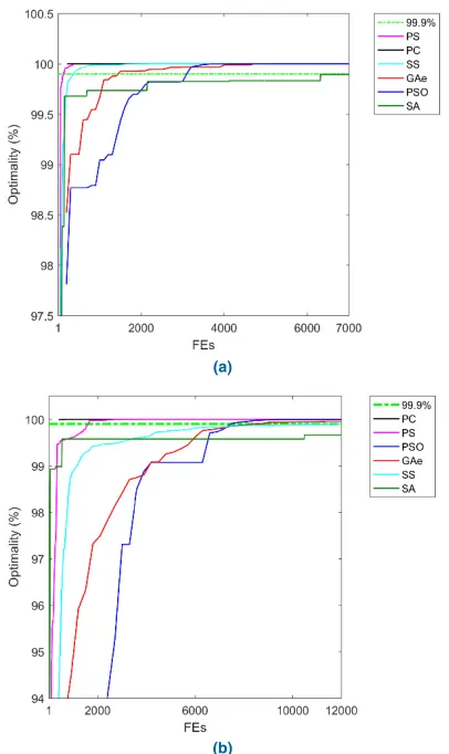
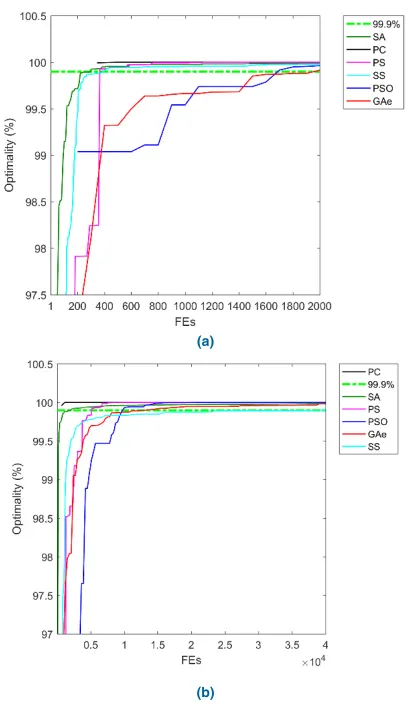
FIGURE 5. Typical optimality of each DFO in optimizing the unimodal quartic problemf1.(a)D=10. (b)D=30.
best performance overall, although PC, PS and PSO all win on three benchmarks. From both the 10-D and 30-D tests, it can be seen that PC offers the best overall performance, and should hence be recommended for uni-modal problems. Further, PC also offers the most ‘linear’ polynomial time (although NP), shown in the last column, whilst SS and SA are the worst. As expected, PSO and GAe are also rela-tively ‘polynomial’. On contrast, SS and SA offer the lowest performance with the highest overheads, and hence should be avoided for this type of problems. Fig. 5 depicts typical optimality convergence of the best point in a ‘generation’.
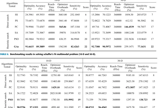
2) VARYING LANDSCAPE n-D MULTIMODAL PROBLEMf2
This function has multiple extrema in [0, π]D and is a more challenging problem than the unimodal problem. Table 5 summarizes the test results and Fig. 6 shows the convergence traces of the optimizers. It is seen that none of the algorithms was able to reach the optimality of 99.9% in
[image:6.576.39.272.447.528.2]TABLE 4. Benchmarking results in solving the quartic unimodal problem (10-D and 30-D).
[image:7.576.37.544.304.649.2]TABLE 5. Benchmarking results in solving the varying landscape multimodal problem (10-D and 30-D).
TABLE 6. Benchmarking results in solving schaffer’s F6 multimodal problem (10-D and 30-D).
3) EXPANDED SCAFFER’S F6 MULTIMODAL PROBLEMf3
Table 6 summarizes the test results on this problem. Fig. 7 shows the convergence traces of the algorithms. It can be seen that PSO delivered consistently good and the overall
[image:7.576.35.537.484.661.2]TABLE 7. Benchmarking results in solving the hybrid problem (10-D and 30-D).
FIGURE 6. Typical optimality of each DFO in optimizing the varying landscape problemf2.(a)D=10. (b)D=30.
FIGURE 7. Typical optimality of each DFO in optimizing Schaffer’s F6 problemf3. (a)D=30. (b)D=30.
multimodal problems. It is also seen that the optimality of PC was relatively inconsistent with that on the previous multimodal problem, indicating it is likely to be trapped in a local optimum when the complexity of the problem increases.
4) HYBRID PROBLEMf4
FIGURE 8. Typical optimality of each DFO in optimizing the hybrid problemf4. (a)D=10. (b)D=30.
in Fig. 8 shows that PC has similar convergence tendency to the case inf3. Combining Figs. 7 and 8, we can conclude that PC is suitable for simple or unimodal functions, but not for multimodal functions. Asf4 has relatively more straightfor-ward troughs, PS and PC were able to exploit the search well.
C. COMPARISON ON INDIVIDUAL BENCHMARKS 1) OPTIMALITY
Table 8 presents the scores and ranking of the six algorithms on optimality in solving problemsf1tof4in 10-D and 30-D, where a higher score is assigned to better optimality. The algorithms are then ranked from 1 to 6 based on their total scores in solving all the problems, where 1 being the top rank. Overall, when a good optimal solution is needed, GAe is seen the best method to use.
2) ACCURACY
[image:9.576.54.259.62.415.2]Table 9 ranks the six algorithms on their accuracy. It can be seen that, when applied to f2,f3 andf4, the algorithms did equally well in both 10-D and 30-D. Although different in 10-D and 30-D onf1, SS and SA did worse than the other four algorithms. For accuracy, GAe is seen the most suitable
TABLE 8.Scores and ranking on optimality.
[image:9.576.299.535.373.477.2]TABLE 9.Scores and ranking on accuracy.
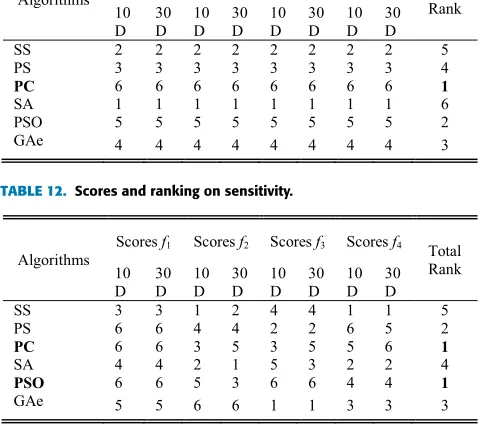
TABLE 10.Scores and ranking on reach time.
for multimodal problems such asf2,f3, whilst PS and PSO for unimodal and simple problems such asf1andf4.
3) REACH TIME
Table 10 ranks on reach time, wheref2andf3 are missing, as none of the algorithms could reach 99.9% accuracy by the end of the predefined maximum number of FEs. When the purpose of optimization is to find a relatively fast converging solution, the PC is seen most suitable for unimodal and simple problems.
4) OPTIMIZER OVERHEADS
FIGURE 9. A simplified decision tree for selecting a DFO. Note that if an application requires optimizing its structure, the GAe is recommended, since its encoding capability permits optimization of structures and categories, in addition to numerical parameters of a structure. Relevantly, the GAe is recommended for global search offline together with PC for local tuning or rapid learning and adaptation online.
[image:10.576.36.276.393.606.2]TABLE 11. Scores and ranking on optimizer overheads.
TABLE 12. Scores and ranking on sensitivity.
5) SENSITIVITY
Table 12 ranks on sensitivity. It can be seen that PC and PSO would be the choice, if low sensitivity is a major concern in practice.
D. QUICK GUIDE TO SELECTING A DFO
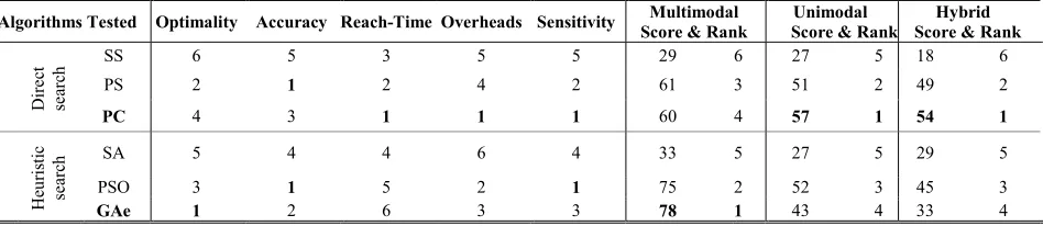
To suit their application at hand most, the user could select a DFO using its individual benchmark ranking or the over-all ranking on amalgamated scores in Table 13, which is
summarized from Tables 8-12. For example, if the objective space or optimality is of a paramount importance for the application, then the GAe would be the No. 1 tool for it, as well as for a potentially multimodal or relatively complex problem.
If the decision space or accuracy is the goal, then PSO and PS would be the choice, with the former being more suit-able for a multimodal problem and the latter unimodal. For unknown modality or a relatively simple problem, PC would provide a rapid assessment on possible effects of applying optimization to the problem at hand.
If the application is rather unknown, however, it is rec-ommended that it could first be treated as a multimodal problem for global optimization using the GAe, which will take a longer time, and then as a unimodal problem for local optimization using PC, which will be a lot quicker. From the above analysis, a visual guide is provided as a decision tree in Fig. 9.
V. CASE STUDY - PARTICLE FILTERING
A. THE STOCHASTIC NONLINEAR FILTER
The particle filter (PF) uses a set of particles (i.e., samples) to represent the posterior distribution of a stochastic process given partial observations. It is a Monte Carlo algorithm to solve Bayesian estimation and signal processing problems. Second to the median filter, the PF is so far the most widely used nonlinear filter [20] following the Sequential Impor-tance Resampling algorithm developed by Gorden [21].
A PF can be formalized in the generic form of a nonlinear system:
TABLE 13. Individual and overall performance rankings of heuristic and direct search DFO for structural and numerical optimization.
zk =h(xk,vk−1) (25) wherexk andzk are the state variables and observations at
timek, respectively,xk ∈ Rnx,zk ∈ Rnz,nxandnzare the
dimensions ofxkandzk, respectively,f (·)andh(·)represent
the system and observation functions, respectively, uk−1 ∈ Rnxis the system noise andvk ∈Rnzis the observation noise
of given distributions, anduk−1andvk−1are independent of the past and current states. In addition,vk may be
indepen-dent ofuk−1. Denote the state and observation sequences by x0:k = x0,···,xk andz1:k = z1,···,zk , respectively. The
initial distribution p(x0)is known a priori.
The objective of the PF is recursively to estimate the posterior density p(x0:k|z1:k)of the state x0:k based on all
available measurements z1:k. A recursive derivation of the
posterior density is given by the Bayesian theorem when new observations arrive:
p(x0:k|z1:k)=p(x0:k−1|z1:k−1)
p(zk|xk)p(xk|xk−1)
p(zk|z1:k−1)
(26)
where the conditional density p(zk|z1:k−1)is a normalizing constant. Eq. (26) can be simplified to:
p(x0:k|z1:k)∝p(x0:k−1|z1:k−1)p(zk|xk)p(xk|xk−1) (27) where∝means proportional to [19].
The above formulas are intractable integrals to an analytic solution forp(x0:k|z1:k). The PF hence uses the Monte Carlo
methods to translate the integral problem into a cumulative particle probability transition. It approximates p(x0:k|z1:k)
with a mass of particlesxi0:k(i=1,· · · ,N), in whichN is the particle number,xi
0is a set of initial particles drawn from
p(x0).
To estimate the posterior distribution of the transition, the PF uses an ‘importance sampling’ technique to sample particles first [22]:
q(x0:k|z1:k)=q(x0:k−1|z1:k−1)q(xk|x0:k−1,z1:k) (28)
Accordingly, the weights of the particles are termed the importance weight. Un-normalized weights can then be writ-ten as
wik = p(x0:k|z1:k)
q(x0:k|z1:k)
∝wik−1p zk
|xik
p xik|xik−1
qxik|xi0:k−1,z 1:k
(29)
wherewik is the importance weight. Denote the normalized
wikasw˜ik. If the importance distribution satisfies
q xk|x0:k−1,z1:k
=q(xk|xk−1,zk) (30)
Then
˜
wik∝ ˜wik−1p zk
|xikp xik|xik−1
qxik|xik−1,z k
(31)
Consequently, the posterior densityp(xk|z1:k)can be formu-lated as:
p(xk|z1:k)≈
XN
i=1w˜
i kδ
xk−xik
(32)
whereδ (·)is the Dirac delta [22].
Despite that the PF is the second most successful nonlinear filter, serious challenges exist. One is the particle impover-ishment problem, which due to most particles sharing a few distinct values cause a loss of diversity and estimation.
To improve, a larger number of optimization algorithms have been applied to particle filtering.
B. TESTS OF MATLAB DFOs AND VERIFICATION
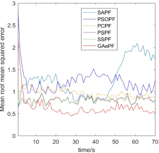
In this case study, tests of all the six DFO are conducted to select the most suitable DFO for the PF and to verify the benchmark guide. In the following, the SS, PS, PC, SA, PSO and GAe versions of the PF are termed SSPF, PSPF, PCPF, SAPF, PSOPF and GAePF, respectively.
A PF application is likely a multimodal or complex prob-lem, the nature of which could be unknown to the user. The tests will be under the representative conditions described in [18], which are widely adopted owing to their strong nonlinearity [22]–[24].
The test formulation is given by:
xk =1+sin(wπk)+φ1xk−1+vk (33)
zk = (
φ2xk2+nk k≤30
φ3xk−2+nk k>30
(34)
FIGURE 10. Mean RMSE errors with observation times for 100 simulations, comparing MATLAB DFOs.
number of generations is set as G = 20. In the GAePF, the crossover probability and the mutation probability are the usual 0.8 and 0.2, respectively. Other parameters of other four DFOs are the same as the above. All particle filters used N =100 particles. The experiment was repeated for
M =100 Monte Carlo simulations to evaluate the perfor-mance of the six potential DFO PF algorithms.
1) ACCURACY ANALYSIS ON STATE ESTIMATIONS
The following three metrics were used to evaluate the perfor-mance of the six PF algorithms:
rmse=
r
1
T
XT
k=1 xk− ˆxk
2
(35)
rmse=
s
1
M
XM
m=1
1
T
XT
k=1 x
m k − ˆxkm
2
(36)
rmse0 =
r
1
M
XM
m=1 x
m k − ˆx
m k
2
(37)
wherermseis the root mean squared error, its mean isrmse,
rmse0is thermseoverMsimulations with a given observation time,xkmis the real state at timekfor them-th simulation, and
ˆ
xkmis the estimated state.
Given the observation time, the meanrmsevalues at every observation in 100 simulations of the six algorithms are shown in Fig. 10. As expected from the DFO guide of Fig. 9, the mean rmse values of the GAePF are seen the lowest. Unexpectedly, however, the PSOPF has shown poor perfor-mance. Investigation into this has uncovered that the PSO in MATLAB does not make a set of the best population available for access after optimization, but the PF algorithm needs a set of particles.
[image:12.576.78.237.66.219.2]To further verify the results, the mean estimationrmseof the six algorithms in different numbers of simulations are shown in Fig. 11, where N = 100 and M = 100. This corroborates the observations from Fig. 10 above, confirming that the GAe is indeed the best DFO for such an unknown application as recommended in the guide.
[image:12.576.299.535.304.394.2]FIGURE 11. Mean RMSE errors vs. the number of simulations for 100 simulations, comparing MATLAB DFOs.
TABLE 14.Mean RMSE and runtime.
2) UTILIZATION OF PARTICLES AND RUNTIME
The meansrmseand average runtime with the total obser-vation time T of the algorithms over 100 simulations are compared in Table 14 for bothN = 100 andN = 300 at
G = 20. It can be seen that the GAePF achieved a lower
rmsefor just 100 particles than all the other algorithms even with 300 particles. As a result, the GAePF also demanded a shorter runtime. In other words, the use of the GAe needed fewer particles to achieve more accurate estimations for the PF application. These tests also confirm that the PF problem, looking relatively complex, is indeed a relatively multimodal problem.
VI. CONCLUSIONS
In this paper, a set of five criteria for benchmarking numerical optimization algorithms are first presented. These bench-marks reflect performance of DFOs on various aspects. Not only have the existing optimality, accuracy and convergence benchmarks been expanded in this paper, but also have the optimizer overheads and sensitivity benchmarks developed to enrich the existing evaluation criteria for practical numerical optimization applications.
overall best for unimodal and simple hybrid problems, whilst the GAe is the overall best for multimodal and relatively complex problems.
To provide a guide for practical engineers to decide rapidly which of the DFOs would be the most suitable for their application at hand without the need for in-depth knowl-edge of the DFO algorithms themselves, a scoring system and a decision tree are provided in this paper. If optimality (the objective space) is of the paramount importance to the application, such as in a competition, the GAe would be the choice. If accuracy (the decision space) or sensitivity is the main concern, such as for tolerating manufacturing inaccuracies of a design-optimized product, then PSO or PS would be the choice. If the application is rather unknown, it is recommended that it could first be treated as a multimodal problem for global optimization using the GAe, which will take a longer time, and then, if desired, as a unimodal problem for local optimization using PC, which will be a lot quicker.
With the guide of the ranks and the decision tree, all the six optimizers have been applied to the nonlinear problem of par-ticle filtering. The GAe is confirmed being better equipped to deal with such a relatively challenging optimization problem. For future work, benchmarking and selection criteria will be extended to multi-target optimization problems.
REFERENCES
[1] The Mathworks, Company Overview. Accessed: May 1, 2019. [Online]. Available: https://www.mathworks.com/content/dam/mathworks/tag-team/Objects/c/company-fact-sheet-8282v18.pdf
[2] V. M. Lo, ‘‘Heuristic algorithms for task assignment in distributed sys-tems,’’IEEE Trans. Comput., vol. 37, no. 11, pp. 1384–1397, Nov. 1988. [3] A. R. Conn, K. Scheinberg, and L. N. Vicente,Introduction to
Derivative-Free Optimization. Philadelphia, PA, USA: SIAM, 2009, p. 277. [4] M. J. D. Powell, ‘‘Direct search algorithms for optimization calculations,’’
Acta Numerica, vol. 7, pp. 287–336, Nov. 1998.
[5] Y. Sun, X. Wang, Y. Chen, and Z. Liu, ‘‘A modified whale optimiza-tion algorithm for large-scale global optimizaoptimiza-tion problems,’’Expert Syst. Appl., vol. 114, pp. 563–577, Dec. 2018.
[6] O. Mersmann, M. Preuss, H. Trautmann, B. Bischl, and C. Weihs, ‘‘Ana-lyzing the BBOB results by means of benchmarking concepts,’’Evol. Comput., vol. 23, no. 1, pp. 161–185, 2015.
[7] L. Li, Y. Chen, Q. Liu, J. Lazic, W. Luo, and Y. Li, ‘‘Benchmarking and evaluating MATLAB derivative-free optimisers for single-objective applications,’’ inProc. ICIC, Liverpool, U.K., 2017, pp. 75–88. [8] Q. Chen, B. Liu, Q. Zhang, J. Liang, P. Suganthan, and B. Qu,
‘‘Prob-lem definitions and evaluation criteria for CEC 2015 special session on bound constrained single-objective computationally expensive numerical optimization,’’ NTU, Singapore, Tech. Rep., 2014.
[9] J. Liang, B. Qu, and P. Suganthan, ‘‘Problem definitions and evaluation criteria for the CEC 2014 special session and competition on single objec-tive real-parameter numerical optimization,’’ NTU, Singapore, Tech. Rep., 2013.
[10] W. Feng, T. Brune, L. Chan, M. Chowdhury, C. Kuek, and Y. Li, ‘‘Bench-marks for testing evolutionary algorithms,’’ inProc. Asia–Pacific Conf. Control Meas., GanSu, China, 1998, pp. 134–138.
[11] K. C. Tan and Y. Li, ‘‘Performance-based control system design automation via evolutionary computing,’’Eng. Appl. Artif. Intell., vol. 14. no. 4, pp. 473–486, 2001.
[12] L. Li, C. Zhang, Z. Li, and Y. Li, ‘‘Particle filter with Lamarckian inheri-tance for nonlinear filtering,’’ inProc. IEEE Congr. Evol. Comput. (CEC), Vancouver, BC, Canada, Jul. 2016, pp. 2852–2857.
[13] Powell on MathWorks. Accessed: Mar. 29, 2017. [Online].
Available: https://cn.mathworks.com/matlabcentral/fileexchange/15072-unconstrained-optimization-using-powell/content/powell.m
[14] Z.-H. Zhan, J. Zhang, Y. Li, and H. S.-H. Chung, ‘‘Adaptive particle swarm optimization,’’IEEE Trans. Syst., Man, Cybern. B, Cybern., vol. 39, no. 6, pp. 1362–1381, Dec. 2009.
[15] X. Yao, Y. Liu, and G. Lin, ‘‘Evolutionary programming made faster,’’
IEEE Trans. Evol. Comput., vol. 3, no. 2, pp. 82–102, Jul. 1999. [16] Z. Michalewicz, ‘‘Evolution strategies and other methods,’’ inGenetic
Algorithms+Data Structures=Evolution Programs, 1st ed. New York, NY, USA: Springer, 1996, pp. 159–177.
[17] J.-M. Renders and H. Bersini, ‘‘Hybridizing genetic algorithms with hill-climbing methods for global optimization: Two possible ways,’’ in
Proc. IEEE 1st Conf. Evol. Comput., IEEE World Congr. Comput. Intell., Orlando, FL, USA, Jun. 1994, pp. 312–317.
[18] Q. Yang, W.-N. Chen, T. Gu, and H. Zhang, ‘‘Segment-based predomi-nant learning swarm optimizer for large-scale optimization,’’IEEE Trans. Cybern., vol. 47, no. 9, pp. 2896–2910, Sep. 2017.
[19] G. E. P. Box, J. S. Hunter, and W. G. Hunter,Statistics for Experimenters: Design, Innovation, and Discovery, 2nd ed. New York, NY, USA: Wiley, 2005.
[20] A. Banerjee and P. Burlina, ‘‘Efficient particle filtering via sparse ker-nel density estimation,’’ IEEE Trans. Image Process., vol. 19, no. 9, pp. 2480–2490, Sep. 2010.
[21] N. J. Gordon, D. J. Salmond, and A. F. M. Smith, ‘‘Novel approach to nonlinear/non-Gaussian Bayesian state estimation,’’IEE Proc. F (Radar Signal Process.), vol. 140, pp. 107–113, Apr. 1993.
[22] C. Musso, N. Oudjane, and F. Le Gland, ‘‘Improving regularised particle filters,’’ inSequential Monte Carlo Methods in Practice. New York, NY, USA: Springer, 2001, pp. 247–271.
[23] T. Higuchi, ‘‘Monte Carlo filter using the genetic algorithm operators,’’
J. Stat. Comput. Simul., vol. 59, no. 1, pp. 1–23, Feb. 1997.
[24] N. M. Kwok, G. Fang, and W. Zhou, ‘‘Evolutionary particle filter: Re-sampling from the genetic algorithm perspective,’’ inProc. IEEE/RSJ Int. Conf. IROS, Edmonton, AB, Canada, Aug. 2005, pp. 2935–2940.
LIN LI(M’17) received the B.S. degree in elec-tronic information engineering from Anhui Agri-culture University, Hefei, China, in 2009, and the Ph.D. degree in signal information process-ing from Harbin Engineerprocess-ing University, Harbin, China, in 2016.
In 2015, she was a Postgraduate Visiting Researcher with the University of Glasgow, U.K. Since 2017, she has been a Postdoctoral Research Fellow with the Industry 4.0 Artificial Intelligence Laboratory, Dongguan University of Technology, Dongguan, China, and also with the South China University of Technology, Guangzhou, China. Her research interests include signal processing, target tracking, computational intelligence, optimization algorithms, and their applications.
ALFREDO ALAN FLORES SALDIVARwas born in Saltillo, Coahuila, Mexico, in 1984. He received the B.Eng. degree in industrial and systems engi-neering from the Autonomous University of the North East, Coahuila, in 2009, the M.S. degree in advanced manufacturing systems from the Mex-ican Corporation of Materials Research, Saltillo, in 2013, and the Ph.D. degree in mechanical engi-neering from the University of Glasgow, Glasgow, U.K., in 2018.
YUN BAI (M’17) received the B.S. and M.S. degrees in environmental engineering from the Chongqing Technology and Business University, Chongqing, China, in 2008 and 2011, respectively, and the Ph.D. degree in civil engineering from Chongqing University, Chongqing, in 2014.
He is currently a Postdoctoral Research Fel-low with the Dongguan University of Technology, Dongguan, China. His current research interests include intelligent computing and its applications to engineering system management, and reliability management.
YI CHEN (M’10–SM’17) received the B.Sc. degree from Chongqing Engineering University, China, the M.Sc. degree from Chongqing sity, China, and the Ph.D. degree from the Univer-sity of Glasgow, U.K.
His research interests are in artificial intelli-gence, high-performance computing, evolution-ary computation, robotic systems, and automation. He is one of the editorial board members of a number of international journals and has been one of the guest editors for five special issues.
Dr. Chen is a member of the IMechE, AAAI, IET, AIAA, and ASME, and a fellow of the HEA. He is also a Chartered Engineer in the U.K.
QUNFENG LIU received the B.S. and M.S. degrees from the Huazhong University of Science and Technology, in 1999 and 2002, respectively, and the Ph.D. degree from Hunan University, China, in 2011.
He is currently an Associate Professor with the School of Computer Science and Network Secu-rity, Dongguan University of Technology, China. His current research interests include global opti-mization, evolutionary computation, and machine learning.
YUN LI (S’87–M’90–SM’17) received the B.S. degree in electronics science from Sichuan Univer-sity, Chengdu, China, in 1984, the M.E. degree in electronic engineering from the Electronic Science and Technology of China (UESTC), Chengdu, China, in 1987, and the Ph.D. degree in parallel computing and control from the University of Strathclyde, Glasgow, U.K., in 1990.
In 1989, he was a Control Engineer with the U.K. National Engineering Laboratory. In 1990, he was a Postdoctoral Research Engineer with the Industrial Systems and Control Ltd. From 1991 to 2018, he was a Lecturer, Senior Lecturer, and Professor with the University of Glasgow and has served as its Founding Director of the University of Glasgow Singapore. He is currently a Professor with the Dongguan University of Technology, Dongguan, China, and also a part-time Professor with the University of Strathclyde, Glasgow, U.K. He has published over 260 papers, one of which is the most popular article every month in the IEEE TRANSACTIONSCONTROLSYSTEMSTECHNOLOGYand another the 3rd in the IEEE TRANSACTIONSSYSTEMS, MAN, ANDCYBERNETICS
-PARTB: CYBERNETICS. He is the author of the popular interactive evolutionary
algorithm (EA) courseware EA_demo (http://i4ai.org/EA-demo/) published online first, in 1997. His current research interest includes artificial intelli-gence for Industry 4.0.
Dr. Li is an Associate Editor of the IEEE TRANSACTIONSEVOLUTIONARY
COMPUTATION and of the IEEE TRANSACTIONS EMERGING TOPICS IN
COMPUTATIONALINTELLIGENCE. He is a Chartered Engineer and an FRSA in