Assessment and development of stability enhancing methods for dynamically changing power hardware-in-the-loop simulations

ASSESSMENT AND DEVELOPMENT OF STABILITY ENHANCING METHODS FOR

DYNAMICALLY CHANGING POWER HARDWARE-IN-THE-LOOP SIMULATIONS

Efren GUILLO-SANSANO1_{, Mazheruddin H. SYED}1_{, Andrew J. ROSCOE}2 _{and Graeme M. BURT}1

1_{University of Strathclyde – UK} 2_{Siemens Gamesa Renewable Energy– UK} [email protected] [email protected]

ABSTRACT

In this paper, to extend the range of Power hardware-in-the-loop (PHIL) simulations into dynamically changing systems, i.e., setups where during the test scenario the ratio of impedance of the simulation and hardware under test changes, an adaptive Ideal Transformer Method (ITM) interface algorithm is proposed. The method incorporates voltage and current sources at both sides of the interface (simulation and hardware), a switch and an online stability assessment monitoring for the operation of the switch. Two different study cases have been developed for the assessment of the performance of the proposed adaptive ITM interface algorithm in a simulation environment. First, a simple test case with a variable resistive hardware under test has been carried out, followed by a case with a series resistive and inductive load. From the results obtained from the assessment of the proposed interface algorithm, a guideline for performing stability assessments of PHIL simulations in dynamically changing scenarios in a more accurate manner is also provided.

INTRODUCTION

A power hardware-in-the-loop (PHIL) implementation comprises a virtually simulated network implemented within a digital real-time simulator (DRTS), a hardware component referred to as the hardware under test (HUT), and the power interface used for interconnecting both the subsystems as shown in Figure 1 [1]. The interface between hardware and software present in PHIL simulations introduces non ideal behaviors and dynamics, such as gains and latencies that typically do not exist in electrically coupled systems [2]. For facilitating the interconnection of the two subsystems with the power interface an interface algorithm (IA) is required. These IAs are not only used for PHIL applications, but also typically used for the coupling of different sections of a simulated system with different time-steps, as multi-rate real time simulations or co-simulation environments [3].

The different IAs used for PHIL applications are not always applicable for all the testing scenarios, and depending on the test characteristics, the IA is selected accordingly [4].

PHIL is typically used for component testing, however there is also more and more interest in cyber-physical systems and systems level testing [3], [5-8], which will require of more flexible interfaces with increased

reliability under a large variety of scenarios.

This paper proposes a new adaptive interfacealgorithm for dynamically changing PHIL simulations that improves the stability compared with other interface algorithms described in the literature. Results from the comparison are presented and analysed under different scenarios with varying loading conditions and load types. Furthermore, from the results of the proposed algorithm a guideline for performing stability assessments of PHIL simulations on a more accurate form is presented. This will prevent misunderstandings and inaccurate stability assessments.

INTERFACE ALGORITHMS FOR PHIL

An interface can be defined as a shared boundary with information exchanges between the involved sections. For PHIL implementations the boundary is at the electrical point of common coupling (PCC) of the HUT with the Digital Real Time Simulator (DRTS). The specification of this interface for PHIL is defined as the interface algorithm. This specification includes the type, quantity, and function of the interconnection circuits and the type and form of signals to be exchanged by these circuits [9]. An analysis of different interface algorithms proposed in the literature for PHIL simulations has been presented in [4] and [10]. From this analysis, the Ideal Transformer Method (ITM) and Damping Impedance Method (DIM) interface algorithms are suggested as the most reliable ones for performing PHIL simulations in terms of stability and accuracy. Accordingly, most of the PHIL research and validation experiments are performed using these algorithms. In this paper, a novel interface algorithm based on the ITM IA has been developed and analysed against ITM and DIM IAs. Therefore, first an introduction of these conventional methods is required.

Ideal Transformer Method (ITM)

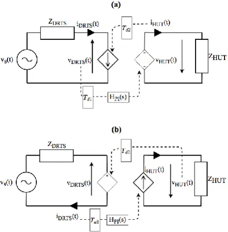
Depending on the signal to be amplified at the hardware side, two different types of ITM IA exist. First, the voltage-type ITM (V-ITM) in which the voltage is amplified at the hardware PCC. The other option would be to amplify the

current rather than the voltage, this known as the current-type ITM (I-ITM). Both algorithms are presented in Fig. 2, where ZDRTS and ZHUT are the simulation and hardware impedance respectively, HPI is the transfer function of the power interface and Td1 and Td2 represent the time delay present in the feedforward and feedback path of the PHIL configuration.

For achieving stable PHIL simulations with ITM IAs, the ratio |ZDRTS(s)|/|ZHUT(s)| is conventionally assumed to be the decisive characteristic, which must be less than 1 for V- ITM interfaces and larger than 1 for I- ITM [1].

Damping impedance method (DIM)

The DIM IA has been previously presented and analyzed in [1]. The electrical schematic of this IA is presented in Fig. 3. In comparison with the ITM methods presented, it can be observed that a damping impedance (Z*) is added in this case into the simulation side alongside a voltage source. This approach aims at emulating the impedance of the HUT and when this impedance matches exactly the HUT impedance, the system would always be stable under ideal conditions (no delays or inaccuracies).

Therefore, the accuracy and stability of a simulation performed with a DIM IA depends on an accurate measurement of the impedance of the HUT, which requires to be continuously updated in real time. This can be difficult to be obtained for complex network components and even more in a real time basis.

ADAPTIVE ITM INTERFACE ALGORITHM

To improve the stability of PHIL simulations, an adaptive-ITM IA is proposed, combining both I-adaptive-ITM and V-adaptive-ITM IAs. Based on their conventional stability conditions,

when a PHIL scenario becomes unstable for one of them, the other ITM variant would be stable. These conventional stability conditions are dependent on the ratio of impedance magnitudes [1], [11-13]. Therefore if the stability conditions are known, and the parameters that influence the stability conditions can be monitored, similarly to the DIM algorithm, then the developed IA could be adapted to remain always stable.

The schematic of the adaptive-ITM IA is presented in Fig. 4. In contrast with the previously presented ITM methods, in this case both voltage source and current source are present on both sides of the interface. The choice of which source is to be used by the IA is made with the use of a switch at each side of the interface controlled by the output of the stability conditions, in this case the calculated impedance ratio.

With the general approach to find the stability conditions of ITM IAs, the switch for changing the interfaces will be operated with a signal activated by the ratio |ZDRTS(s)|/|ZHUT(s)| as:

𝑠𝑤𝑖𝑡𝑐ℎ = {𝑉𝐼𝑇𝑀, 𝑖𝑓

|ZDRTS(s)| |ZHUT(s)| < 1 𝐼𝐼𝑇𝑀, 𝑜𝑡ℎ𝑒𝑟𝑤𝑖𝑠𝑒

(1)

As a result, the simulation would be stable if the ratio of impedance magnitudes is calculated accurately and the transition between interfaces is performed smoothly without transients. Similarly to the DIM algorithm, adaptive-ITM also requires of the identification of the HUT impedance, nevertheless the DIM requires of a very precise identification as the accuracy depends on it, while for the adaptive-ITM the precision has a more limited effect into the accuracy. Crucially, the need for a real-time adjustment of the simulation impedance is not required in this case.

Figure 3. Diagram of DIM interface algorithm

CASE STUDY

Variable resistance with X

=X

=0

A variable resistor is selected as the HUT for this experiment. This variable resistor allows for the study of different scenarios that can challenge the stability of PHIL simulations. A controlled voltage source along with an impedance will be the simulated part of the system, the voltage source will be able to introduce dynamics into the simulation in order to study the effect that it can have into the overall accuracy and stability of the simulation. A first simulation has been performed with a source impedance value of 1Ω and a variable resistor set to decrease its value from 30Ω to 0.1Ω therefore forcing the ratio of impedances |ZDRTS(s)|/|ZHUT(s)| to go out of its condition for stability. During this transition both voltage and current ITM methods become unstable due to that change in impedance magnitude. The DIM IA along with the Adaptive-ITM IA are implemented with the same impedance calculation algorithm. From the simulation, shown in Fig. 5, it is shown that the DIM IA at the time of the change of impedance creates a large transient that the Adaptive-ITM method is not producing. So, for this scenario it is shown that the adaptive-ITM algorithm would be much more accurate and stable than any of the other methods presented previously.

Figure 3. a) Comparison of interface algorithms results under variable resistance and b) measured impedance values, from V-ITM to I-V-ITM

In order to test the stability and accuracy of the interfaces a similar scenario is studied where the HUT impedance will be increasing its value from ZHUT =5Ω until it has a larger value than the impedance at the simulation side that is set to ZDRTS =10Ω in this case. This would cause instability on the regular ITM interface algorithms. However, as it is shown in Fig. 6 the adaptive ITM algorithm manages to maintain the stability of the simulation, although a small ripple is present at the time of switching from I-ITM to V-ITM compared with the DIM algorithm in this case. The DIM algorithm appears to handle this scenario in a very stable and accurate manner in comparison with the previous one.

Figure 4. Comparison of interface algorithms results under variable resistance and b) measured impedance values, from I-ITM to V-I-ITM

Variable resistance in presence of inductances

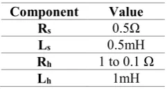
A second test has been carried out where the HUT and the simulation impedance are both a series RL component. Similarly to the previous scenario, the resistor on the HUT will be dynamically varied for assessing the performance of the proposed interface. The components used for this scenario are presented in Table 1.

Table 1. PHIL components values

Component Value Rs 0.5Ω Ls 0.5mH Rh 1 to 0.1 Ω

Lh 1mH

The adaptive-ITM IA has yielded positive results for a resistive HUT as the ratio of impedances when XDRTS=XHUT=0 is still prevailing; however, when more complex HUT are analysed, the identified condition is no longer accurate. Therefore, in contrast with conventional PHIL stability assessments performed with Nyquist and Bode criterions, and as already suggested by [14] and [15], the stability of ITM methods does not always depends on the impedance ratio |ZDRTS(s)|/|ZHUT(s)|, but only for resistive scenarios. Accordingly, detailed stability study of the ITM method is required for providing more informed decisions on the transition between interfaces and achieving stable PHIL simulations.

ACCURATE STABILITY ASSESSMENT

In contrast with conventional stability assessment procedures for PHIL simulations, in which Bode or Nyquist stability criterion are used and a pure resistive impedance is assumed, in this case stability assessment based on the Routh-Hurwitz criterion is preferred. The main difference of the stability assessment performed here with respect to conventional assessments is that the impedances are not assumed purely resistive (not frequency dependant), as when inductors or capacitors are part of the system, their frequency dependency will be changing the poles and zeros placement and accordingly modifying the stability of the system.

Routh-Hurwitz criterion will give a necessary and sufficient condition for the stability of a linear feedback system. Although simplification of non-linear components is required, it allows to define the stability of the system based on the variables of the system, avoiding the need for identifying system poles and zeros, as would be the case of the Nyquist or Bode criterion conventionally used for PHIL simulations.

A simplified control loop diagram of a PHIL implementation with V-ITM interface and RL impedances on both sides of the system is presented in Fig. 8 for the thorough evaluation of the stability with Routh-Hurwitz, where:

𝐻𝐷𝑅𝑇𝑆(𝑠) = 𝑅𝑠+ 𝑠𝐿𝑠 (2)

𝐻𝐻𝑈𝑇(𝑠) =

1 𝑅ℎ+ 𝑠𝐿ℎ

(3)

with the transfer function of the time delay approximated with a first order Pade approximation for its conversion into a rational function, represented by:

𝐻𝑑𝑒𝑙𝑎𝑦(𝑠) = 𝑒−𝑠𝑇𝑑≈

−𝑇𝑑

2 𝑠 + 1 𝑇𝑑

2 𝑠 + 1

(4)

The Routh-Hurwitz stability criterion is applied to different arrangements of HUT (resistor (Rh), inductor (Lh) and capacitor (Ch)), when the simulation impedance is composed of a resistor (Rs) in series with an inductor (Ls) (as it is a typical configuration of reduced power systems). As a result, stability conditions required for the different arrangements of the HUT are presented in Table 2. It can be observed that when capacitive components are added to the HUT, stability tends to be at risk (except for the series RLC combination).

This results are in contrast with the inaccurately commonly defined stability condition of impedance magnitude ratio |ZDRTS(s)|/|ZHUT(s)| larger or smaller than 1 for ITM IAs. This is only accurate when HUT and DRTS impedances are only resistive. If an inductive component is present the ratio of inductors will usually be more decisive than the ratio of impedances, as in that case even if the ratio of impedances met the condition, the system would still be unstable if the ratio of inductors is not met.

Table 2. Stability conditions

ZDRTS ZHUT Stability Condition Rs Ls Rh Rh > Rs

Rs Ls Lh

1) Lh > Ls 2) 𝑅𝑠<

2(𝐿ℎ+𝐿𝑠) 𝑇_𝑑 Rs Ls Ch Unstable

Rs Ls Rh Lh

1) Lh > Ls 2) 𝑅𝑠 < 𝑅ℎ+

2(𝐿ℎ+𝐿𝑠) 𝑇_𝑑

Rs Ls Rh Ch Unstable

Figure 5. a) Measured impedance b) comparison of interface algorithms results under variable impedance

Rs Ls Rh Lh Ch

1) Lh > Ls 2) 𝑅𝑠< 𝑅ℎ+

2(𝐿ℎ+𝐿𝑠) 𝑇_𝑑 3) (Td +2ChRh+2ChRs) · (2Lh+2Ls+RhTd +RsTd) >

2Td(Lh−Ls)

Rs Ls Rh || Lh Unstable

Rs Ls Rh || Ch Unstable

Rs Ls Rh || Lh || Ch Unstable

Accordingly, if the values of inductance, capacitance and time delay can be calculated in real time, then the stability conditions could be assessed and the interface selected accordingly.

CONCLUSIONS

A novel IA, the adaptive-ITM, has been presented based on previous stability analysis performed in the literature, in which the ratio of impedances was shown as the deciding stability condition. However, with the evaluation of the adaptive-ITM it has been identified that this condition is only valid for a system where only resistive impedances are present. Therefore the application of A-ITM is possible when such a case is present in a PHIL simulation or when all the other parameters are also identified.

This has led to a more precise stability assessment in which the Routh-Hurwitz stability criteria has been used. As a result, detailed stability conditions for any type of load and V-ITM interface have been obtained in which the impedance ratio is no longer the stability condition and where the most important parameter affecting the stability of PHIL simulations with ITM IA are the inductances of the simulation and HUT.

Acknowledgments

The work in this paper has been supported by the European Commission, under the Horizon 2020 project ERIGrid (grant no: 654113).

REFERENCES

[1] W. Ren, M. Steurer, and T. L. Baldwin. “Improve the stability and the accuracy of power hardware-in-the-loop simulation by selecting appropriate interface algorithms”. In: IEEE Transactions on Industry Applications (2008), pp. 1286–1294.

[2] Guillo-Sansano, E.; H. Syed, M.; J. Roscoe, A.; M. Burt, G. “Initialization and Synchronization of Power Hardware-In-The-Loop Simulations: A Great Britain Network Case Study”, Energies 2018, 11, 1087. [3] M. Stevic et al., "Multi-site European framework for

real-time co-simulation of power systems," in IET GTD, vol. 11, 4126-4135, 2017.

[4] Brandl, R. “Operational Range of Several Interface Algorithms for Different Power Hardware-In-The-Loop Setups”, Energies 2017, 10, 1946.

[5] Lundstrom, B.; Palmintier, B.; Rowe, D.; Ward, J.; Moore, T.: 'Trans-oceanic remote power hardware-in-the-loop: multi-site hardware, integrated controller, and electric network co-simulation', IET GTD, 2017, 11, (18), p. 4688-4701.

[6] B. Palmintier, B. Lundstrom, S. Chakraborty, T. Williams, K. Schneider and D. Chassin, "A Power Hardware-in-the-Loop Platform With Remote Distribution Circuit Cosimulation," in IEEE Transactions on Industrial Electronics, vol. 62, no. 4, pp. 2236-2245, April 2015.

[7] A. Monti et al., "A Global Real-Time Superlab: Enabling High Penetration of Power Electronics in the Electric Grid," in IEEE Power Electronics Magazine, vol. 5, no. 3, pp. 35-44, Sept. 2018.

[8] J. L. Cale et al., "Mitigating Communication Delays in Remotely Connected Hardware-in-the-Loop Experiments," in IEEE Transactions on Industrial Electronics, vol. 65, (12), pp. 9739-9748, Dec. 2018. [9] The Authoritative Dictionary of IEEE Standards

Terms, SeventhEdition, in IEEE Std 100-2000 , vol., no., pp.1-1362, Dec. 11, 2000.

[10] Ren, W., Steurer, M., and Baldwin, T. L., 2008, “Improve the stability and the accuracy of power hardware-in-the-loop simulation by selecting appropriate interface algorithms”, IEEE Transactions on Industry Applications, 44(4), 1286-1294.

[11] M. Dargahi, A. Ghosh, and G. Ledwich. “Stability synthesis of power hardware-in-the-loop (PHIL) simulation”. In: IEEE PES GM. October 2014. [12] C. S. Edrington et al. “Role of Power Hardware in the

Loop in Modeling and Simulation for Experimentation in Power and Energy Systems”. In: Proceedings of the IEEE 103.12 (2015), 2401–2409. [13] F. Lehfuß, G. Lauss, and T. Strasser. “Implementation

of a multi-rating interface for Power-Hardware-in-the-Loop simulations”. In: IECON Proceedings. 2012, pp. 4777–4782.

[14] M. Hong et al. “A method to stabilize a power hardware-in-the-loop simulation of inductor coupled systems”. In: Int. Conf. on Power Systems Transients (IPST2009) in Kyoto, Japan (2009).